[go: up one dir, main page]

Next Issue
Volume 9, July-2
Previous Issue
Volume 9, June-2


Mathematics, Volume 9, Issue 13 (July-1 2021) – 128 articles

Cover Story (view full-size image): 
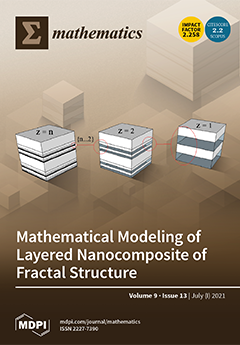
A model of a layered, hierarchically constructed composite is presented, the structure of which demonstrates the properties of similarity at different scales. For the proposed model of the composite, fractal analysis was carried out, including an assessment of the permissible range of scales, calculation of fractal capacity, Hausdorff and Minkovsky dimensions, and calculation of the Hurst exponent. The maximum and minimum sizes at which fractal properties are observed are investigated, and a quantitative assessment of the complexity of the proposed model is carried out. A software package is developed that allows one to calculate the fractal characteristics of hierarchically constructed composite media. A qualitative analysis of the calculated fractal characteristics is also carried out. View this paper
  • Issues are regarded as officially published after their release is announced to the table of contents alert mailing list.
  • You may sign up for e-mail alerts to receive table of contents of newly released issues.
  • PDF is the official format for papers published in both, html and pdf forms. To view the papers in pdf format, click on the "PDF Full-text" link, and use the free Adobe Reader to open them.
Order results
Result details
Section
Select all
Export citation of selected articles as:
15 pages, 61065 KiB  
Article
Numerical Modeling of Face Shield Protection against a Sneeze
by Ainara Ugarte-Anero, Unai Fernandez-Gamiz, Iñigo Aramendia, Ekaitz Zulueta and Jose Manuel Lopez-Guede
Mathematics 2021, 9(13), 1582; https://doi.org/10.3390/math9131582 - 5 Jul 2021
Cited by 10 | Viewed by 3528
Abstract
The protection provided by wearing masks has been a guideline worldwide to prevent the risk of COVID-19 infection. The current work presents an investigation that analyzes the effectiveness of face shields as personal protective equipment. To that end, a multiphase computational fluid dynamic [...] Read more.
The protection provided by wearing masks has been a guideline worldwide to prevent the risk of COVID-19 infection. The current work presents an investigation that analyzes the effectiveness of face shields as personal protective equipment. To that end, a multiphase computational fluid dynamic study based on Eulerian–Lagrangian techniques was defined to simulate the spread of the droplets produced by a sneeze. Different scenarios were evaluated where the relative humidity, ambient temperature, evaporation, mass transfer, break up, and turbulent dispersion were taken into account. The saliva that the human body generates was modeled as a saline solution of 8.8 g per 100 mL. In addition, the influence of the wind speed was studied with a soft breeze of 7 km/h and a moderate wind of 14 km/h. The results indicate that the face shield does not provide accurate protection, because only the person who is sneezed on is protected. Moreover, with a wind of 14 km/h, none of the droplets exhaled into the environment hit the face shield, instead, they were deposited onto the neck and face of the wearer. In the presence of an airflow, the droplets exhaled into the environment exceeded the safe distance marked by the WHO. Relative humidity and ambient temperature play an important role in the lifetime of the droplets. Full article
(This article belongs to the Special Issue Computational Mechanics in Engineering Mathematics)
Show Figures

Figure 1

Figure 1
<p>Evaporation of a single pure water droplet under different environment conditions, environment temperature of 293.15 K, particle temperature 310.15 K, and different droplet sizes (1 µm, 10 µm, and 100 µm).</p>
Full article ">Figure 2
<p>Freely falling water droplets based on the study of Hamey (1982). Particle sizes of 110 µm and 115 µm, environment temperature 293 K, particle temperature 289 K, and 70% relative humidity.</p>
Full article ">Figure 3
<p>Human geometry: (<b>a</b>) Human body (1.8 m tall); (<b>b</b>) Face shield in detail.</p>
Full article ">Figure 4
<p>Position of the mouth at 1.5 m: (<b>a</b>) The same height as the human with the face shield, 1.6 m; (<b>b</b>) A difference of height of 20 cm; (<b>c</b>) Geometry of the mouth (DM = 40 mm and dm = 20 mm) to simulate a sneeze.</p>
Full article ">Figure 5
<p>Mesh distribution, the block (<span class="html-fig-inline" id="mathematics-09-01582-i001"> <img alt="Mathematics 09 01582 i001" src="/mathematics/mathematics-09-01582/article_deploy/html/images/mathematics-09-01582-i001.png"/></span>) indicates the mouth of the individual that has the virus and sneezes: (<b>a</b>) The mesh in the domain when the mouths were at the same height; (<b>b</b>) The mesh in the domain when the mouths were at different heights (20 cm difference).</p>
Full article ">Figure 6
<p>The distribution of the droplets size at t = 0.4 s and t = 2.5 s when the environment temperature was 15 °C and the relative humidity was 40%.</p>
Full article ">Figure 7
<p>The distribution of the droplets size at t = 2.5 s when the environment temperature was 15 °C. Comparison between RH = 40% and RH = 60%.</p>
Full article ">Figure 8
<p>The distribution of the droplets size at t = 2.5 s when the relative humidity was 40%. Comparison between T<sub>e</sub> = 15 °C and T<sub>e</sub> = 25 °C.</p>
Full article ">Figure 9
<p>The velocity that the droplets acquire when the relative humidity is 60% and the ambient temperature is 15 °C, at different wind speeds (soft breeze of 7 km/h and moderate wind of 14 km/h). When there was a soft breeze, the droplets reached the other human in 0.62 s and 0.55 s when the human mouths were at the same height and with a height difference of 20 cm, respectively. When there was a moderate wind speed, the droplets reached the other human in 0.0.75 s and 0.45 s when the human mouths were at the same height and with a height difference of 20 cm, respectively.</p>
Full article ">Figure 10
<p>Area of the face shield that protects the human at a 40% RH and T<sub>e</sub> = 25 °C. (<b>a</b>) Wind speed of 7 km/h and the mouths at the same height; (<b>b</b>) Wind speed of 14 km/h and the mouths at the same height; (<b>c</b>) Wind speed of 7 km/h and the mouths with a height difference of 20 cm; (<b>d</b>) Wind speed of 14 km/h and the mouths with a height difference of 20 cm.</p>
Full article ">Figure 11
<p>Mass of the droplets entering the face shield at 40% RH and T<sub>e</sub> = 25 °C. (<b>a</b>) Wind speed of 7 km/h and the mouths at the same height; (<b>b</b>) Wind speed of 14 km/h and the mouths at the same height; (<b>c</b>) Wind speed of 7 km/h and the mouths with a height difference of 20 cm; (<b>d</b>) Wind speed of 14 km/h and the mouths with a height difference of 20 cm.</p>
Full article ">
17 pages, 4110 KiB  
Article
Hybrid Optimization Based Mathematical Procedure for Dimensional Synthesis of Slider-Crank Linkage
by Alfonso Hernández, Aitor Muñoyerro, Mónica Urízar and Enrique Amezua
Mathematics 2021, 9(13), 1581; https://doi.org/10.3390/math9131581 - 5 Jul 2021
Cited by 6 | Viewed by 2495
Abstract
In this paper, an optimization procedure for path generation synthesis of the slider-crank mechanism will be presented. The proposed approach is based on a hybrid strategy, mixing local and global optimization techniques. Regarding the local optimization scheme, based on the null gradient condition, [...] Read more.
In this paper, an optimization procedure for path generation synthesis of the slider-crank mechanism will be presented. The proposed approach is based on a hybrid strategy, mixing local and global optimization techniques. Regarding the local optimization scheme, based on the null gradient condition, a novel methodology to solve the resulting non-linear equations is developed. The solving procedure consists of decoupling two subsystems of equations which can be solved separately and following an iterative process. In relation to the global technique, a multi-start method based on a genetic algorithm is implemented. The fitness function incorporated in the genetic algorithm will take as arguments the set of dimensional parameters of the slider-crank mechanism. Several illustrative examples will prove the validity of the proposed optimization methodology, in some cases achieving an even better result compared to mechanisms with a higher number of dimensional parameters, such as the four-bar mechanism or the Watt’s mechanism. Full article
(This article belongs to the Special Issue Applied Mathematics to Mechanisms and Machines)
Show Figures

Figure 1

Figure 1
<p>Slider-crank mechanism with 5 dimensional parameters.</p>
Full article ">Figure 2
<p>Two possible configurations for the same input.</p>
Full article ">Figure 3
<p>Slider-crank mechanism with 8 dimensional parameters.</p>
Full article ">Figure 4
<p>Error function for a point <math display="inline"><semantics> <mi>i</mi> </semantics></math> evaluated at [0,2π).</p>
Full article ">Figure 5
<p>Generated trajectory and prescribed point (red).</p>
Full article ">Figure 6
<p>Flowchart of the hybrid optimization scheme.</p>
Full article ">Figure 7
<p>Example 1. Desired trajectory.</p>
Full article ">Figure 8
<p>Example 1: best multi-start solution for slider-crank, E = 0.0073.</p>
Full article ">Figure 9
<p>Example 1: comparison to other multi-start solution (multi-start no. 10), E = 0.0227.</p>
Full article ">Figure 10
<p>Example 2: optimal solution for: (<b>a</b>) four-bar and (<b>b</b>) slider-crank mechanism.</p>
Full article ">Figure 11
<p>(<b>a</b>) Watt’s mechanism optimal solution from [<a href="#B41-mathematics-09-01581" class="html-bibr">41</a>]; (<b>b</b>) optimal solution for slider-crank mechanism.</p>
Full article ">
9 pages, 1840 KiB  
Article
A Modified Recursive Regularization Factor Calculation for Sparse RLS Algorithm with l1-Norm
by Junseok Lim, Keunhwa Lee and Seokjin Lee
Mathematics 2021, 9(13), 1580; https://doi.org/10.3390/math9131580 - 5 Jul 2021
Cited by 2 | Viewed by 2029
Abstract
In this paper, we propose a new calculation method for the regularization factor in sparse recursive least squares (SRLS) with l1-norm penalty. The proposed regularization factor requires no prior knowledge of the actual system impulse response, and it also reduces computational [...] Read more.
In this paper, we propose a new calculation method for the regularization factor in sparse recursive least squares (SRLS) with l1-norm penalty. The proposed regularization factor requires no prior knowledge of the actual system impulse response, and it also reduces computational complexity by about half. In the simulation, we use Mean Square Deviation (MSD) to evaluate the performance of SRLS, using the proposed regularization factor. The simulation results demonstrate that SRLS using the proposed regularization factor calculation shows a difference of less than 2 dB in MSD from SRLS, using the conventional regularization factor with a true system impulse response. Therefore, it is confirmed that the performance of the proposed method is very similar to that of the existing method, even with half the computational complexity. Full article
(This article belongs to the Special Issue Advances in Computational and Applied Mathematics)
Show Figures

Figure 1

Figure 1
<p>MSD comparison in <span class="html-italic">N</span> = 64 for S = 2, 4, 8, and 16 when applying the proposed regularization factor to the <math display="inline"><semantics> <msub> <mi>l</mi> <mn>1</mn> </msub> </semantics></math>-RLS: (<b>a</b>) MSD at S = 2 (<b>b</b>) MSD at S = 4 (<b>c</b>) MSD at S = 8 (<b>d</b>) MSD at S = 16 (-▹-: <math display="inline"><semantics> <msub> <mi>l</mi> <mn>1</mn> </msub> </semantics></math>-RLS using the proposed regularization factor without the true system impulse response, -×-: <math display="inline"><semantics> <msub> <mi>l</mi> <mn>1</mn> </msub> </semantics></math>-RLS using the conventional regularization factor with the true system impulse response, -∘-: <math display="inline"><semantics> <msub> <mi>l</mi> <mn>1</mn> </msub> </semantics></math>-RLS from [<a href="#B19-mathematics-09-01580" class="html-bibr">19</a>], -⋄-: conventional RLS without considering sparsity, -▿-: <math display="inline"><semantics> <msub> <mi>l</mi> <mn>1</mn> </msub> </semantics></math>-IWF from [<a href="#B21-mathematics-09-01580" class="html-bibr">21</a>]).</p>
Full article ">Figure 2
<p>MSD comparison in <span class="html-italic">N</span> = 256 for S = 2, 4, 8, and 16 when applying the proposed regularization factor to the <math display="inline"><semantics> <msub> <mi>l</mi> <mn>1</mn> </msub> </semantics></math>-RLS: (<b>a</b>) MSD at S = 2 (<b>b</b>) MSD at S = 4 (<b>c</b>) MSD at S = 8 (<b>d</b>) MSD at S = 16 (-▹-: <math display="inline"><semantics> <msub> <mi>l</mi> <mn>1</mn> </msub> </semantics></math>-RLS using the proposed regularization factor without the true system impulse response, -×-: <math display="inline"><semantics> <msub> <mi>l</mi> <mn>1</mn> </msub> </semantics></math>-RLS using the conventional regularization factor with the true system impulse response, -∘-: <math display="inline"><semantics> <msub> <mi>l</mi> <mn>1</mn> </msub> </semantics></math>-RLS from [<a href="#B19-mathematics-09-01580" class="html-bibr">19</a>], -⋄-: conventional RLS without considering sparsity, -▿-: <math display="inline"><semantics> <msub> <mi>l</mi> <mn>1</mn> </msub> </semantics></math>-IWF from [<a href="#B21-mathematics-09-01580" class="html-bibr">21</a>]).</p>
Full article ">Figure 2 Cont.
<p>MSD comparison in <span class="html-italic">N</span> = 256 for S = 2, 4, 8, and 16 when applying the proposed regularization factor to the <math display="inline"><semantics> <msub> <mi>l</mi> <mn>1</mn> </msub> </semantics></math>-RLS: (<b>a</b>) MSD at S = 2 (<b>b</b>) MSD at S = 4 (<b>c</b>) MSD at S = 8 (<b>d</b>) MSD at S = 16 (-▹-: <math display="inline"><semantics> <msub> <mi>l</mi> <mn>1</mn> </msub> </semantics></math>-RLS using the proposed regularization factor without the true system impulse response, -×-: <math display="inline"><semantics> <msub> <mi>l</mi> <mn>1</mn> </msub> </semantics></math>-RLS using the conventional regularization factor with the true system impulse response, -∘-: <math display="inline"><semantics> <msub> <mi>l</mi> <mn>1</mn> </msub> </semantics></math>-RLS from [<a href="#B19-mathematics-09-01580" class="html-bibr">19</a>], -⋄-: conventional RLS without considering sparsity, -▿-: <math display="inline"><semantics> <msub> <mi>l</mi> <mn>1</mn> </msub> </semantics></math>-IWF from [<a href="#B21-mathematics-09-01580" class="html-bibr">21</a>]).</p>
Full article ">
16 pages, 601 KiB  
Article
Efficiency Analysis with Educational Data: How to Deal with Plausible Values from International Large-Scale Assessments
by Juan Aparicio, Jose M. Cordero and Lidia Ortiz
Mathematics 2021, 9(13), 1579; https://doi.org/10.3390/math9131579 - 5 Jul 2021
Cited by 17 | Viewed by 4096
Abstract
International large-scale assessments (ILSAs) provide several measures as a representation of educational outcomes, the so-called plausible values, which are frequently interpreted as a representation of the ability range of students. In this paper, we focus on how this information should be incorporated into [...] Read more.
International large-scale assessments (ILSAs) provide several measures as a representation of educational outcomes, the so-called plausible values, which are frequently interpreted as a representation of the ability range of students. In this paper, we focus on how this information should be incorporated into the estimation of efficiency measures of student or school performance using data envelopment analysis (DEA). Thus far, previous studies that have adopted this approach using data from ILSAs have used only one of the available plausible values or an average of all of them. We propose an approach based on the fuzzy DEA, which allows us to consider the whole distribution of results as a proxy of student abilities. To assess the extent to which our proposal offers similar results to those obtained in previous studies, we provide an empirical example using PISA data from 2015. Our results suggest that the performance measures estimated using the fuzzy DEA approach are strongly correlated with measures calculated using just one plausible value or an average measure. Therefore, we conclude that the studies that decide upon using one of these options do not seem to be making a significant error in their estimates. Full article
(This article belongs to the Special Issue Economics of Education: Quantitative Methods for Educational Policies)
Show Figures

Figure 1

Figure 1
<p>Examples of kernel functions for the PVMATH variable.</p>
Full article ">
23 pages, 1510 KiB  
Article
Automatic Group Organization for Collaborative Learning Applying Genetic Algorithm Techniques and the Big Five Model
by Oscar Revelo Sánchez, César A. Collazos and Miguel A. Redondo
Mathematics 2021, 9(13), 1578; https://doi.org/10.3390/math9131578 - 5 Jul 2021
Cited by 5 | Viewed by 2654
Abstract
In this paper, an approach based on genetic algorithms is proposed to form groups in collaborative learning scenarios, considering the students’ personality traits as a criterion for grouping. This formation is carried out in two stages: In the first, the information of the [...] Read more.
In this paper, an approach based on genetic algorithms is proposed to form groups in collaborative learning scenarios, considering the students’ personality traits as a criterion for grouping. This formation is carried out in two stages: In the first, the information of the students is collected from a psychometric instrument based on the Big Five personality model; whereas, in the second, this information feeds a genetic algorithm that is in charge of performing the grouping iteratively, seeking for an optimal formation. The results presented here correspond to the functional and empirical validation of the approach. It is found that the described methodology is useful to obtain groups with the desired characteristics. The specific objective is to provide a strategy that makes it possible to subsequently assess in the context what type of approach (homogeneous, heterogeneous, or mixed) is the most appropriate to organize the groups. Full article
Show Figures

Figure 1

Figure 1
<p>GA general scheme.</p>
Full article ">Figure 2
<p>The main flow of the student group formation process using GA.</p>
Full article ">Figure 3
<p>GA performance.</p>
Full article ">Figure 4
<p>Pre-test results. (<b>a</b>) Computer Programming; (<b>b</b>) Graphic Programming.</p>
Full article ">Figure 5
<p>Post-test results. (<b>a</b>) Computer Programming; (<b>b</b>) Graphic Programming.</p>
Full article ">
12 pages, 3892 KiB  
Article
An Embedding Strategy Using Q-Ary Convolutional Codes for Large and Small Payloads
by Jyun-Jie Wang, Chi-Yuan Lin, Sheng-Chih Yang, Hsi-Yuan Chang and Yin-Chen Lin
Mathematics 2021, 9(13), 1577; https://doi.org/10.3390/math9131577 - 4 Jul 2021
Viewed by 2158
Abstract
Matrix embedding (ME) code is a commonly used steganography technique, which uses linear block codes to improve embedding efficiency. However, its main disadvantage is the inability to perform maximum likelihood decoding due to the high complexity of decoding large ME codes. As such, [...] Read more.
Matrix embedding (ME) code is a commonly used steganography technique, which uses linear block codes to improve embedding efficiency. However, its main disadvantage is the inability to perform maximum likelihood decoding due to the high complexity of decoding large ME codes. As such, it is difficult to improve the embedding efficiency. The proposed q-ary embedding code can provide excellent embedding efficiency and is suitable for various embedding rates (large and small payloads). This article discusses that by using perforation technology, a convolutional code with a high embedding rate can be easily converted into a convolutional code with a low embedding rate. By keeping the embedding rate of the (2, 1) convolutional code unchanged, convolutional codes with different embedding rates can be designed through puncturing. Full article
Show Figures

Figure 1

Figure 1
<p>Block diagram of a binary embedding system.</p>
Full article ">Figure 2
<p>Rate-distortion function.</p>
Full article ">Figure 3
<p>Standard array for the embedding algorithm.</p>
Full article ">Figure 4
<p>3-Ary, constraint length = 4, <math display="inline"><semantics> <mi>η</mi> </semantics></math> = 4.37.</p>
Full article ">Figure 5
<p>3-Ary, constraint length = 5, <math display="inline"><semantics> <mi>η</mi> </semantics></math> = 4.53.</p>
Full article ">Figure 6
<p>5-Ary, constraint length = 4, <math display="inline"><semantics> <mi>η</mi> </semantics></math> = 5.1.</p>
Full article ">Figure 7
<p>7-Ary, constraint length = 4, <math display="inline"><semantics> <mi>η</mi> </semantics></math> = 5.42.</p>
Full article ">Figure 8
<p>7-Ary, constraint length = 5, <math display="inline"><semantics> <mi>η</mi> </semantics></math> = 5.56.</p>
Full article ">Figure 9
<p>5-Ary, constraint length = 3, <math display="inline"><semantics> <mi>η</mi> </semantics></math> = 4.8.</p>
Full article ">Figure 10
<p>5-Ary, constraint length = 5, <math display="inline"><semantics> <mi>η</mi> </semantics></math> = 5.1.</p>
Full article ">Figure 11
<p>Packet form in the application field.</p>
Full article ">Figure 12
<p>Example of the packet form.</p>
Full article ">Figure 13
<p>GUI of the image steganography system.</p>
Full article ">Figure 14
<p>The embedding efficiency between [<a href="#B16-mathematics-09-01577" class="html-bibr">16</a>] and convolutional embedding codes.</p>
Full article ">
21 pages, 21971 KiB  
Article
A Study on the Impact of Linguistic Persuasive Styles on the Sales Volume of Live Streaming Products in Social E-Commerce Environment
by Hanyang Luo, Sijia Cheng, Wanhua Zhou, Sumin Yu and Xudong Lin
Mathematics 2021, 9(13), 1576; https://doi.org/10.3390/math9131576 - 4 Jul 2021
Cited by 54 | Viewed by 14332
Abstract
Live-stream shopping is developing rapidly, but the sales levels of live streaming products vary by different hosts. How to increase the sales volume of live streaming products has become a problem. Consumers’ purchase behavior in live streaming is determined by some subjective factors, [...] Read more.
Live-stream shopping is developing rapidly, but the sales levels of live streaming products vary by different hosts. How to increase the sales volume of live streaming products has become a problem. Consumers’ purchase behavior in live streaming is determined by some subjective factors, and the persuasiveness of linguistic style affects this subjective judgment to a certain extent. Therefore, the persuasiveness of the hosts’ linguistic style will lead to changes in consumers’ purchase intentions, which will affect the sales volume of products sold in the live streaming. Based on Hovland’s persuasion model, Aristotle’s rhetoric skills, text analysis, Latent Dirichlet Allocation (LDA) topic extraction model and grounded theory, this study divides the host’s linguistic persuasive style in the social e-commerce environment into five types: appealing to personality, appealing to logic, appealing to emotion, appealing to reward, and appealing to exaggeration. Combined with the sales volume of the product, we establish a regression model, and obtain the influence results of the host’s various linguistic persuasive styles on the sales of live streaming products. The results show that: the linguistic persuasive style of appealing to personality has the greatest positive impact on the sales volume of live broadcast products, but the linguistic style of appealing to logic has a negative impact. Interestingly, the same linguistic style has different effects for different types of products: the linguistic style of appealing to exaggeration has a negative effect on the sales volume of apparel products, but it has a positive influence on the sales volume of digital electrical products. Therefore, different linguistic styles should be used for different product types. Full article
Show Figures

Figure 1

Figure 1
<p>Research Model.</p>
Full article ">Figure 2
<p>Research procedure based on grounded theory.</p>
Full article ">Figure 3
<p>Schematic diagram of LDA model structure.</p>
Full article ">Figure 4
<p>The number of times the linguistic style is used for various types of goods.</p>
Full article ">Figure 5
<p>Predictive Model (5) first test result.</p>
Full article ">Figure 6
<p>Predictive model (5) second test results. (<b>a</b>) VIF test results of Model 6.; (<b>b</b>) model (5) second test result.</p>
Full article ">Figure 7
<p>VIF test results of Models. (<b>a</b>) VIF test results of Model 7; (<b>b</b>) VIF test results of Model 8; (<b>c</b>) VIF test results of Model 9; (<b>d</b>) VIF test results of Model 10; (<b>e</b>) VIF test results of Model 11; (<b>f</b>) VIF test results of Model 12.</p>
Full article ">Figure 8
<p>Model test results. (<b>a</b>) Model (7) test result; (<b>b</b>) Model (8) test result; (<b>c</b>) Model (9) test result; (<b>d</b>) Model (10) test result; (<b>e</b>) Model (11) test result; (<b>f</b>) Model (12) test result.</p>
Full article ">Figure 8 Cont.
<p>Model test results. (<b>a</b>) Model (7) test result; (<b>b</b>) Model (8) test result; (<b>c</b>) Model (9) test result; (<b>d</b>) Model (10) test result; (<b>e</b>) Model (11) test result; (<b>f</b>) Model (12) test result.</p>
Full article ">
19 pages, 835 KiB  
Article
Application of Induced Preorderings in Score Function-Based Method for Solving Decision-Making with Interval-Valued Fuzzy Soft Information
by Mabruka Ali, Adem Kiliçman and Azadeh Zahedi Khameneh
Mathematics 2021, 9(13), 1575; https://doi.org/10.3390/math9131575 - 4 Jul 2021
Cited by 2 | Viewed by 1915
Abstract
Ranking interval-valued fuzzy soft sets is an increasingly important research issue in decision making, and provides support for decision makers in order to select the optimal alternative under an uncertain environment. Currently, there are three interval-valued fuzzy soft set-based decision-making algorithms in the [...] Read more.
Ranking interval-valued fuzzy soft sets is an increasingly important research issue in decision making, and provides support for decision makers in order to select the optimal alternative under an uncertain environment. Currently, there are three interval-valued fuzzy soft set-based decision-making algorithms in the literature. However, these algorithms are not able to overcome the issue of comparable alternatives and, in fact, might be ignored due to the lack of a comprehensive priority approach. In order to provide a partial solution to this problem, we present a group decision-making solution which is based on a preference relationship of interval-valued fuzzy soft information. Further, corresponding to each parameter, two crisp topological spaces, namely, lower topology and upper topology, are introduced based on the interval-valued fuzzy soft topology. Then, using the preorder relation on a topological space, a score function-based ranking system is also defined to design an adjustable multi-steps algorithm. Finally, some illustrative examples are given to compare the effectiveness of the present approach with some existing methods. Full article
Show Figures

Figure 1

Figure 1
<p>Comparison methods.</p>
Full article ">Figure 2
<p>Nonlinear ordering system.</p>
Full article ">
14 pages, 928 KiB  
Article
A Cascade Deep Forest Model for Breast Cancer Subtype Classification Using Multi-Omics Data
by Ala’a El-Nabawy, Nahla A. Belal and Nashwa El-Bendary
Mathematics 2021, 9(13), 1574; https://doi.org/10.3390/math9131574 - 4 Jul 2021
Cited by 13 | Viewed by 3387
Abstract
Automated diagnosis systems aim to reduce the cost of diagnosis while maintaining the same efficiency. Many methods have been used for breast cancer subtype classification. Some use single data source, while others integrate many data sources, the case that results in reduced computational [...] Read more.
Automated diagnosis systems aim to reduce the cost of diagnosis while maintaining the same efficiency. Many methods have been used for breast cancer subtype classification. Some use single data source, while others integrate many data sources, the case that results in reduced computational performance as opposed to accuracy. Breast cancer data, especially biological data, is known for its imbalance, with lack of extensive amounts of histopathological images as biological data. Recent studies have shown that cascade Deep Forest ensemble model achieves a competitive classification accuracy compared with other alternatives, such as the general ensemble learning methods and the conventional deep neural networks (DNNs), especially for imbalanced training sets, through learning hyper-representations through using cascade ensemble decision trees. In this work, a cascade Deep Forest is employed to classify breast cancer subtypes, IntClust and Pam50, using multi-omics datasets and different configurations. The results obtained recorded an accuracy of 83.45% for 5 subtypes and 77.55% for 10 subtypes. The significance of this work is that it is shown that using gene expression data alone with the cascade Deep Forest classifier achieves comparable accuracy to other techniques with higher computational performance, where the time recorded is about 5 s for 10 subtypes, and 7 s for 5 subtypes. Full article
(This article belongs to the Special Issue Statistical Data Modeling and Machine Learning with Applications)
Show Figures

Figure 1

Figure 1
<p>General structure of the proposed approach.</p>
Full article ">Figure 2
<p>Statistical feature engineering of CNA and CNV data.</p>
Full article ">Figure 3
<p>General structure of the cascade Deep Forest network.</p>
Full article ">
28 pages, 449 KiB  
Article
New Approaches to the General Linearization Problem of Jacobi Polynomials Based on Moments and Connection Formulas
by Waleed Mohamed Abd-Elhameed and Badah Mohamed Badah
Mathematics 2021, 9(13), 1573; https://doi.org/10.3390/math9131573 - 4 Jul 2021
Cited by 9 | Viewed by 1923
Abstract
This article deals with the general linearization problem of Jacobi polynomials. We provide two approaches for finding closed analytical forms of the linearization coefficients of these polynomials. The first approach is built on establishing a new formula in which the moments of the [...] Read more.
This article deals with the general linearization problem of Jacobi polynomials. We provide two approaches for finding closed analytical forms of the linearization coefficients of these polynomials. The first approach is built on establishing a new formula in which the moments of the shifted Jacobi polynomials are expressed in terms of other shifted Jacobi polynomials. The derived moments formula involves a hypergeometric function of the type 4F3(1), which cannot be summed in general, but for special choices of the involved parameters, it can be summed. The reduced moments formulas lead to establishing new linearization formulas of certain parameters of Jacobi polynomials. Another approach for obtaining other linearization formulas of some Jacobi polynomials depends on making use of the connection formulas between two different Jacobi polynomials. In the two suggested approaches, we utilize some standard reduction formulas for certain hypergeometric functions of the unit argument such as Watson’s and Chu-Vandermonde identities. Furthermore, some symbolic algebraic computations such as the algorithms of Zeilberger, Petkovsek and van Hoeij may be utilized for the same purpose. As an application of some of the derived linearization formulas, we propose a numerical algorithm to solve the non-linear Riccati differential equation based on the application of the spectral tau method. Full article
(This article belongs to the Special Issue Polynomial Sequences and Their Applications)
Show Figures

Figure 1

Figure 1
<p>Different errors of Example 1 for different values of α.</p>
Full article ">Figure 2
<p>Different errors of Example 2 for different values of α.</p>
Full article ">
44 pages, 1750 KiB  
Article
A Multi-Depot Vehicle Routing Problem with Stochastic Road Capacity and Reduced Two-Stage Stochastic Integer Linear Programming Models for Rollout Algorithm
by Wadi Khalid Anuar, Lai Soon Lee, Hsin-Vonn Seow and Stefan Pickl
Mathematics 2021, 9(13), 1572; https://doi.org/10.3390/math9131572 - 4 Jul 2021
Cited by 7 | Viewed by 4484
Abstract
A matheuristic approach based on a reduced two-stage Stochastic Integer Linear Programming (SILP) model is presented. The proposed approach is suitable for obtaining a policy constructed dynamically on the go during the rollout algorithm. The rollout algorithm is part of the Approximate Dynamic [...] Read more.
A matheuristic approach based on a reduced two-stage Stochastic Integer Linear Programming (SILP) model is presented. The proposed approach is suitable for obtaining a policy constructed dynamically on the go during the rollout algorithm. The rollout algorithm is part of the Approximate Dynamic Programming (ADP) lookahead solution approach for a Markov Decision Processes (MDP) framed Multi-Depot Dynamic Vehicle Routing Problem with Stochastic Road Capacity (MDDVRPSRC). First, a Deterministic Multi-Depot VRP with Road Capacity (D-MDVRPRC) is presented. Then an extension, MDVRPSRC-2S, is presented as an offline two-stage SILP model of the MDDVRPSRC. These models are validated using small simulated instances with CPLEX. Next, two reduced versions of the MDVRPSRC-2S model (MDVRPSRC-2S1 and MDVRPSRC-2S2) are derived. They have a specific task in routing: replenishment and delivering supplies. These reduced models are to be utilised interchangeably depending on the capacity of the vehicle, and repeatedly during the execution of rollout in reinforcement learning. As a result, it is shown that a base policy consisting of an exact optimal decision at each decision epoch can be obtained constructively through these reduced two-stage stochastic integer linear programming models. The results obtained from the resulting rollout policy with CPLEX execution during rollout are also presented to validate the reduced model and the matheuristic algorithm. This approach is proposed as a simple implementation when performing rollout for the lookahead approach in ADP. Full article
Show Figures

Figure 1

Figure 1
<p>Damage Determination based on Interception on Edge due to Dispersion Radial Circle Representing Earthquake Tremor.</p>
Full article ">Figure 2
<p>Proposed Matheuristic Rollout Concept for One Monte Carlo Episode.</p>
Full article ">Figure A1
<p>Road Network for Instance D3N8S3.</p>
Full article ">Figure A2
<p>Road Network for Instance D4N11S4.</p>
Full article ">Figure A3
<p>Road Network for Instance D5N13S5.</p>
Full article ">Figure A4
<p>Changes in Road Capacity Over Time in Online Simulation and Computation.</p>
Full article ">Figure A5
<p>Total Distance Travelled for Maximum Road Capacity Setting <math display="inline"><semantics> <mrow> <mo>(</mo> <mn>6</mn> <mo>,</mo> <mn>7</mn> <mo>,</mo> <mn>8</mn> <mo>)</mo> </mrow> </semantics></math>: Offline and Online Computation for all Instances based on Model Characteristic.</p>
Full article ">Figure A6
<p>Total Distance Travelled for Maximum Road Capacity Setting <math display="inline"><semantics> <mrow> <mo>(</mo> <mn>2</mn> <mo>,</mo> <mn>3</mn> <mo>,</mo> <mn>4</mn> <mo>)</mo> </mrow> </semantics></math>: Offline and Online Computation for all Instances based on Model Characteristic.</p>
Full article ">Figure A7
<p>Total Travel Time for Maximum Road Capacity Setting <math display="inline"><semantics> <mrow> <mo>(</mo> <mn>6</mn> <mo>,</mo> <mn>7</mn> <mo>,</mo> <mn>8</mn> <mo>)</mo> </mrow> </semantics></math>: Offline and Online Computation for all Instances based on Model Characteristic.</p>
Full article ">Figure A8
<p>Total Travel Time for Maximum Road Capacity Setting <math display="inline"><semantics> <mrow> <mo>(</mo> <mn>2</mn> <mo>,</mo> <mn>3</mn> <mo>,</mo> <mn>4</mn> <mo>)</mo> </mrow> </semantics></math>: Offline and Online Computation for all Instances based on Model Characteristic.</p>
Full article ">Figure A9
<p>Computation Time for Maximum Road Capacity Setting <math display="inline"><semantics> <mrow> <mo>(</mo> <mn>6</mn> <mo>,</mo> <mn>7</mn> <mo>,</mo> <mn>8</mn> <mo>)</mo> </mrow> </semantics></math>: Offline and Online Computation for all Instances based on Model Characteristic.</p>
Full article ">Figure A10
<p>Computation Time for Maximum Road Capacity Setting <math display="inline"><semantics> <mrow> <mo>(</mo> <mn>2</mn> <mo>,</mo> <mn>3</mn> <mo>,</mo> <mn>4</mn> <mo>)</mo> </mrow> </semantics></math>: Offline and Online Computation for all Instances based on Model Characteristic.</p>
Full article ">Figure A11
<p>Total Distance Travelled: Offline and Online based on Model Characteristic and Maximum Road Capacity Setting.</p>
Full article ">Figure A12
<p>Total Travel Time: Offline and Online computation based on Model Characteristic and Maximum Road Capacity Setting.</p>
Full article ">Figure A13
<p>Computation Time: Offline and Online computation based on Model Characteristic and Maximum Road Capacity Setting.</p>
Full article ">Figure A14
<p>Total Distance Travelled for Maximum Road Capacity Setting <math display="inline"><semantics> <mrow> <mo>(</mo> <mn>6</mn> <mo>,</mo> <mn>7</mn> <mo>,</mo> <mn>8</mn> <mo>)</mo> </mrow> </semantics></math> in Online and Offline Computation for all Instances grouped by Model Characteristic.</p>
Full article ">Figure A15
<p>Total Distance Travelled for Maximum Road Capacity Setting <math display="inline"><semantics> <mrow> <mo>(</mo> <mn>2</mn> <mo>,</mo> <mn>3</mn> <mo>,</mo> <mn>4</mn> <mo>)</mo> </mrow> </semantics></math> in Online and Offline Computation for all Instances grouped by Model Characteristic.</p>
Full article ">Figure A16
<p>Total Travel Time for Maximum Road Capacity Setting <math display="inline"><semantics> <mrow> <mo>(</mo> <mn>6</mn> <mo>,</mo> <mn>7</mn> <mo>,</mo> <mn>8</mn> <mo>)</mo> </mrow> </semantics></math> in Online and Offline Computation for all Instances grouped by Model Characteristic.</p>
Full article ">Figure A17
<p>Total Travel Time for Maximum Road Capacity Setting <math display="inline"><semantics> <mrow> <mo>(</mo> <mn>2</mn> <mo>,</mo> <mn>3</mn> <mo>,</mo> <mn>4</mn> <mo>)</mo> </mrow> </semantics></math> in Online and Offline Computation for all Instances grouped by Model Characteristic.</p>
Full article ">Figure A18
<p>Computation Time for Maximum Road Capacity Setting <math display="inline"><semantics> <mrow> <mo>(</mo> <mn>6</mn> <mo>,</mo> <mn>7</mn> <mo>,</mo> <mn>8</mn> <mo>)</mo> </mrow> </semantics></math> in Online and Offline Computation for all Instances grouped by Model Characteristic.</p>
Full article ">Figure A19
<p>Computation Time for Maximum Road Capacity Setting <math display="inline"><semantics> <mrow> <mo>(</mo> <mn>2</mn> <mo>,</mo> <mn>3</mn> <mo>,</mo> <mn>4</mn> <mo>)</mo> </mrow> </semantics></math> in Online and Offline Computation for all Instances grouped by Model Characteristic.</p>
Full article ">Figure A20
<p>Total Distance Travelled in Online and Offline Computation for all Instances grouped by Model Characteristic and Maximum Road Capacity Setting.</p>
Full article ">Figure A21
<p>Total Travel Time in Online and Offline Computation for all Instances grouped by Model Characteristic and Maximum Road Capacity Setting.</p>
Full article ">Figure A22
<p>Computation Time in Online and Offline Computation for all Instances grouped by Model Characteristic and Maximum Road Capacity Setting.</p>
Full article ">
8 pages, 258 KiB  
Article
On the Accuracy of the Generalized Gamma Approximation to Generalized Negative Binomial Random Sums
by Irina Shevtsova and Mikhail Tselishchev
Mathematics 2021, 9(13), 1571; https://doi.org/10.3390/math9131571 - 4 Jul 2021
Cited by 5 | Viewed by 1893
Abstract
We investigate the proximity in terms of zeta-structured metrics of generalized negative binomial random sums to generalized gamma distribution with the corresponding parameters, extending thus the zeta-structured estimates of the rate of convergence in the Rényi theorem. In particular, we derive upper bounds [...] Read more.
We investigate the proximity in terms of zeta-structured metrics of generalized negative binomial random sums to generalized gamma distribution with the corresponding parameters, extending thus the zeta-structured estimates of the rate of convergence in the Rényi theorem. In particular, we derive upper bounds for the Kantorovich and the Kolmogorov metrics in the law of large numbers for negative binomial random sums of i.i.d. random variables with nonzero first moments and finite second moments. Our method is based on the representation of the generalized negative binomial distribution with the shape and exponent power parameters no greater than one as a mixed geometric law and the infinite divisibility of the negative binomial distribution. Full article
(This article belongs to the Special Issue Analytical Methods and Convergence in Probability with Applications)
20 pages, 2052 KiB  
Article
A Robust Approach for Identifying the Major Components of the Bribery Tolerance Index
by Daniel Homocianu, Aurelian-Petruș Plopeanu and Rodica Ianole-Calin
Mathematics 2021, 9(13), 1570; https://doi.org/10.3390/math9131570 - 3 Jul 2021
Cited by 4 | Viewed by 2561
Abstract
The paper aims to emphasize the advantages of several advanced statistical and data mining techniques when applied to the dense literature on corruption measurements and determinants. For this purpose, we used all seven waves of the World Values Survey and we employed the [...] Read more.
The paper aims to emphasize the advantages of several advanced statistical and data mining techniques when applied to the dense literature on corruption measurements and determinants. For this purpose, we used all seven waves of the World Values Survey and we employed the Naive Bayes technique in SQL Server Analysis Services 2016, the LASSO package together with logit and melogit regressions with raw coefficients in Stata 16. We further conducted different types of tests and cross-validations on the wave, country, gender, and age categories. For eliminating multicollinearity, we used predictor correlation matrices. Moreover, we assessed the maximum computed variance inflation factor (VIF) against a maximum acceptable threshold, depending on the model’s R squared in Ordinary Least Square (OLS) regressions. Our main contribution consists of a methodology for exploring and validating the most important predictors of the risk associated with bribery tolerance. We found the significant role of three influences corresponding to questions about attitudes towards the property, authority, and public services, and other people in terms of anti-cheating, anti-evasion, and anti-violence. We used scobit, probit, and logit regressions with average marginal effects to build and test the index based on these attitudes. We successfully tested the index using also risk prediction nomograms and accuracy measurements (AUCROC > 0.9). Full article
Show Figures

Figure 1

Figure 1
<p>Top predictors as identified by using the Naive Bayes algorithm in Microsoft Data Mining add-in for spreadsheets. Source: Own computation in Microsoft Excel 2013 (Data Mining add-in) and SQL Server Analysis Services 2016.</p>
Full article ">Figure 2
<p>Stata processing script for performing derivations needed for cross-validations and starting from the original form of the dependent variable. Source: Own calculation in Stata 16MP 64-bit.</p>
Full article ">Figure 3
<p>Correlation matrices for 10 predictors obtained after performing R and CV LASSO selections and six remaining ones after removing the redundancy. Source: Own calculation in Stata 16MP 64-bit.</p>
Full article ">Figure 4
<p>Stata processing script for deriving the proposed bribe index based on a Scobit regression with resulting coefficients expressed as average marginal effects (<a href="#mathematics-09-01570-t007" class="html-table">Table 7</a>, Model 1). Source: Own calculation in Stata 16MP 64-bit.</p>
Full article ">Figure 5
<p>Two comparable prediction nomograms for estimating the bribery tolerance risk. Source: Own calculations using the nomolog command in Stata 16 MP 64-bit.</p>
Full article ">Figure A1
<p>Schematic representation of the techniques used. Source: The authors’ own projection.</p>
Full article ">
16 pages, 4534 KiB  
Article
A Tool for the Analysis and Characterization of School Mathematical Models
by Jesús Montejo-Gámez, Elvira Fernández-Ahumada and Natividad Adamuz-Povedano
Mathematics 2021, 9(13), 1569; https://doi.org/10.3390/math9131569 - 3 Jul 2021
Cited by 4 | Viewed by 2512
Abstract
This paper shows a tool for the analysis of written productions that allows for the characterization of the mathematical models that students develop when solving modeling tasks. For this purpose, different conceptualizations of mathematical models in education are discussed, paying special attention to [...] Read more.
This paper shows a tool for the analysis of written productions that allows for the characterization of the mathematical models that students develop when solving modeling tasks. For this purpose, different conceptualizations of mathematical models in education are discussed, paying special attention to the evidence that characterizes a school model. The discussion leads to the consideration of three components, which constitute the main categories of the proposed tool: the real system to be modeled, its mathematization and the representations used to express both. These categories and the corresponding analysis procedure are explained and illustrated through two working examples, which expose the value of the tool in establishing the foci of analysis when investigating school models, and thus, suggest modeling skills. The connection of this tool with other approaches to educational research on mathematical modeling is also discussed. Full article
(This article belongs to the Section Engineering Mathematics)
Show Figures

Figure 1

Figure 1
<p>Flux diagram of the analysis procedure for the proposed tool (source: prepared by the authors).</p>
Full article ">Figure A1
<p>Statement of the task “the President’s supporters” translated into English (source: prepared by the authors).</p>
Full article ">Figure A2
<p>Translation into English of the written production for the task “the President’s supporters” analyzed above (source: prepared by the authors).</p>
Full article ">Figure A3
<p>Statement of the task “the play center” translated into English (source: prepared by the authors).</p>
Full article ">Figure A4
<p>Translation into English of the written production for the task “the play center”. Answer to question a) (source: prepared by the authors).</p>
Full article ">Figure A5
<p>Translation into English of the written production for the task “the play center”. Answer to question b) (source: prepared by the authors).</p>
Full article ">Figure A6
<p>Translation into English of the written production for the task “the play center”. Answer to question c) (source: prepared by the authors).</p>
Full article ">
11 pages, 298 KiB  
Article
On the Notion of Reproducibility and Its Full Implementation to Natural Exponential Families
by Shaul K. Bar-Lev
Mathematics 2021, 9(13), 1568; https://doi.org/10.3390/math9131568 - 3 Jul 2021
Viewed by 1557
Abstract
Let F=Fθ:θΘR be a family of probability distributions indexed by a parameter θ and let X1,,Xn be i.i.d. r.v.’s with L(X1)= [...] Read more.
Let F=Fθ:θΘR be a family of probability distributions indexed by a parameter θ and let X1,,Xn be i.i.d. r.v.’s with L(X1)=FθF. Then, F is said to be reproducible if for all θΘ and nN, there exists a sequence (αn)n1 and a mapping gn:ΘΘ,θgn(θ) such that L(αni=1nXi)=Fgn(θ)F. In this paper, we prove that a natural exponential family F is reproducible iff it possesses a variance function which is a power function of its mean. Such a result generalizes that of Bar-Lev and Enis (1986, The Annals of Statistics) who proved a similar but partial statement under the assumption that F is steep as and under rather restricted constraints on the forms of αn and gn(θ). We show that such restrictions are not required. In addition, we examine various aspects of reproducibility, both theoretically and practically, and discuss the relationship between reproducibility, convolution and infinite divisibility. We suggest new avenues for characterizing other classes of families of distributions with respect to their reproducibility and convolution properties . Full article
15 pages, 10412 KiB  
Article
Graph Theory for Primary School Students with High Skills in Mathematics
by Rocío Blanco and Melody García-Moya
Mathematics 2021, 9(13), 1567; https://doi.org/10.3390/math9131567 - 3 Jul 2021
Cited by 4 | Viewed by 3388
Abstract
Graph theory is a powerful representation and problem-solving tool, but it is not included in present curriculum at school levels. In this study we perform a didactic proposal based in graph theory, to provide students useful and motivational tools for problem solving. The [...] Read more.
Graph theory is a powerful representation and problem-solving tool, but it is not included in present curriculum at school levels. In this study we perform a didactic proposal based in graph theory, to provide students useful and motivational tools for problem solving. The participants, who were highly skilled in mathematics, worked on map coloring, Eulerian cycles, star polygons and other related topics. The program included six sessions in a workshop format and four creative sessions where participants invented their own mathematical challenges. Throughout the experience they applied a wide range of strategies to solve problems, such as look for a pattern, counting strategies or draw the associated graph, among others. In addition, they created as challenges the same type of problems posed in workshops. We conclude that graph theory successfully increases motivation of participants towards mathematics and allows the appearance and enforcement of problem-solving strategies. Full article
(This article belongs to the Special Issue Research on Powerful Ideas for Enriching School Mathematical Learning)
Show Figures

Figure 1

Figure 1
<p>Basic graphs. Examples of (<b>a</b>) graph; (<b>b</b>) planar graph; (<b>c</b>) nonplanar graph; (<b>d</b>) Eulerian graph; (<b>e</b>) non-Eulerian graph; (<b>f</b>) Eulerian graph, but non-Hamiltonian graph; (<b>g</b>) Hamiltonian graph, non-Eulerian graph.</p>
Full article ">Figure 2
<p>First attempt of coloring the map of Spain. Drawing made by participant: (<b>a</b>) A3; (<b>b</b>) A6; (<b>c</b>) A4.</p>
Full article ">Figure 3
<p>First attempt of coloring the map of Spain. Drawing made by participant: (<b>a</b>) A1; (<b>b</b>) A2 (orange is yellow); (<b>c</b>) A5; (<b>d</b>) A7.</p>
Full article ">Figure 4
<p>Failed attempt of Eulerian cycle. Drawing made by participant: (<b>a</b>) A1; (<b>b</b>) A4; (<b>c</b>) A6.</p>
Full article ">Figure 5
<p>Example of Eulerian cycle. Drawing made by participant: (<b>a</b>) A2; (<b>b</b>) A3; (<b>c</b>) A5; (<b>d</b>) A7.</p>
Full article ">Figure 6
<p>Star polygons. Drawing made by participant: (<b>a</b>) A2 (similar to the one made by A1); (<b>b</b>) A3.</p>
Full article ">Figure 7
<p>Star polygons. Drawing made by participant: (<b>a</b>) A4; (<b>b</b>) A5; (<b>c</b>) A6; (<b>d</b>) A7.</p>
Full article ">Figure 8
<p>Counting strategies. Drawing made by participant: (<b>a</b>) A6; (<b>b</b>) A1.</p>
Full article ">Figure 9
<p>Counting strategies. Drawing made by participant: (<b>a</b>) A5; (<b>b</b>) A2; (<b>c</b>) A3; (<b>d</b>) A7; (<b>e</b>) A4.</p>
Full article ">Figure 10
<p>Tracing Eulerian cycles. Drawing made by participant: (<b>a</b>) A3; (<b>b</b>) A5; (<b>c</b>) A4; (<b>d</b>) A6; (<b>e</b>) A7.</p>
Full article ">Figure 11
<p>Köningsberg bridges. Drawing made by participant: (<b>a</b>) A7; (<b>b</b>) A6; (<b>c</b>) A5; (<b>d</b>) A3; (<b>e</b>) A4.</p>
Full article ">Figure 12
<p>Graphs associated with Köningsberg bridges. Drawing made by participant: (<b>a</b>) A6; (<b>b</b>) A7; (<b>c</b>) A5; (<b>d</b>) A3; (<b>e</b>) A4.</p>
Full article ">Figure 13
<p>Chess routes with a knight. Drawing made by participant: (<b>a</b>) A5; (<b>b</b>) A7; (<b>c</b>) A3; (<b>d</b>) A4; (<b>e</b>) A6.</p>
Full article ">Figure 14
<p>Chess routes. Drawing made by participant: (<b>a</b>) A5 using a rook; (<b>b</b>) A3 using a rook; (<b>c</b>) A7 using the queen; (<b>d</b>) A4 using a rook; (<b>e</b>) A6 using the king.</p>
Full article ">
18 pages, 343 KiB  
Article
Local Dynamics of Logistic Equation with Delay and Diffusion
by Sergey Kashchenko
Mathematics 2021, 9(13), 1566; https://doi.org/10.3390/math9131566 - 3 Jul 2021
Cited by 4 | Viewed by 2389
Abstract
The behavior of all the solutions of the logistic equation with delay and diffusion in a sufficiently small positive neighborhood of the equilibrium state is studied. It is assumed that the Andronov–Hopf bifurcation conditions are met for the coefficients of the problem. Small [...] Read more.
The behavior of all the solutions of the logistic equation with delay and diffusion in a sufficiently small positive neighborhood of the equilibrium state is studied. It is assumed that the Andronov–Hopf bifurcation conditions are met for the coefficients of the problem. Small perturbations of all coefficients are considered, including the delay coefficient and the coefficients of the boundary conditions. The conditions are studied when these perturbations depend on the spatial variable and when they are time-periodic functions. Equations on the central manifold are constructed as the main results. Their nonlocal dynamics determines the behavior of all the solutions of the original boundary value problem in a sufficiently small neighborhood of the equilibrium state. The ability to control the dynamics of the original problem using the phase change in the perturbing force is set. The numerical and analytical results regarding the dynamics of the system with parametric perturbation are obtained. The asymptotic formulas for the solutions of the original boundary value problem are given. Full article
(This article belongs to the Special Issue Recent Advances in Differential Equations and Applications)
11 pages, 1294 KiB  
Article
SIAM—Colombia MMC: A Challenge-Based Math Modeling Learning Strategy
by Rafael Alberto Méndez-Romero, Diana H. Bueno-Carreño, Carlos Díez-Fonnegra and Johan Manuel Redondo
Mathematics 2021, 9(13), 1565; https://doi.org/10.3390/math9131565 - 3 Jul 2021
Cited by 1 | Viewed by 3399
Abstract
The math modeling challenge CoSIAM is a competition based on interdisciplinary collaborative work challenges. This research seeks to demonstrate the value of this type of challenge-based competition as a learning strategy outside the classroom. Based on data, we conducted a qualitative study on [...] Read more.
The math modeling challenge CoSIAM is a competition based on interdisciplinary collaborative work challenges. This research seeks to demonstrate the value of this type of challenge-based competition as a learning strategy outside the classroom. Based on data, we conducted a qualitative study on the perception of the participants in the last three versions of the mathematical modeling challenge, in terms of the learning achieved, the benefits of their participation, the knowledge and skills they brought into play, and the change in their conception of modeling. The participants were undergraduate and graduate students in mathematics and other areas, from several Colombian and Mexican universities. The research yielded results in three directions. The first is related to the advantages and limitations of teamwork, the second explores the learning that arises from this experience, and the third is oriented to the disciplinary knowledge mobilized for the solution of this type of problematic situation. The study allowed concluding, among other issues, that learning based on interdisciplinary problem solving, formulated from a global perspective, enhances the acquisition of valuable skills for the participants. Full article
Show Figures

Figure 1

Figure 1
<p>The main words that students associate with mathematical modeling.</p>
Full article ">Figure 2
<p>Sankey diagram for emerging categories.</p>
Full article ">
22 pages, 555 KiB  
Article
Nonlinear Dynamics of the Introduction of a New SARS-CoV-2 Variant with Different Infectiousness
by Gilberto Gonzalez-Parra and Abraham J. Arenas
Mathematics 2021, 9(13), 1564; https://doi.org/10.3390/math9131564 - 3 Jul 2021
Cited by 6 | Viewed by 3304
Abstract
Several variants of the SARS-CoV-2 virus have been detected during the COVID-19 pandemic. Some of these new variants have been of health public concern due to their higher infectiousness. We propose a theoretical mathematical model based on differential equations to study the effect [...] Read more.
Several variants of the SARS-CoV-2 virus have been detected during the COVID-19 pandemic. Some of these new variants have been of health public concern due to their higher infectiousness. We propose a theoretical mathematical model based on differential equations to study the effect of introducing a new, more transmissible SARS-CoV-2 variant in a population. The mathematical model is formulated in such a way that it takes into account the higher transmission rate of the new SARS-CoV-2 strain and the subpopulation of asymptomatic carriers. We find the basic reproduction number R0 using the method of the next generation matrix. This threshold parameter is crucial since it indicates what parameters play an important role in the outcome of the COVID-19 pandemic. We study the local stability of the infection-free and endemic equilibrium states, which are potential outcomes of a pandemic. Moreover, by using a suitable Lyapunov functional and the LaSalle invariant principle, it is proved that if the basic reproduction number is less than unity, the infection-free equilibrium is globally asymptotically stable. Our study shows that the new more transmissible SARS-CoV-2 variant will prevail and the prevalence of the preexistent variant would decrease and eventually disappear. We perform numerical simulations to support the analytic results and to show some effects of a new more transmissible SARS-CoV-2 variant in a population. Full article
(This article belongs to the Section Mathematical Biology)
Show Figures

Figure 1

Figure 1
<p>Diagram of the COVID-19 mathematical model (<a href="#FD1-mathematics-09-01564" class="html-disp-formula">1</a>). This shows the transition of individuals between epidemiological classes. <math display="inline"><semantics> <mrow> <mi>S</mi> <mo>(</mo> <mi>t</mi> <mo>)</mo> </mrow> </semantics></math> is the susceptible class, <math display="inline"><semantics> <mrow> <msub> <mi>E</mi> <mrow> <mn>1</mn> <mo>,</mo> <mn>2</mn> </mrow> </msub> <mrow> <mo>(</mo> <mi>t</mi> <mo>)</mo> </mrow> </mrow> </semantics></math> are the two classes of latent individuals for the two SARS-CoV-2 variants, <math display="inline"><semantics> <mrow> <msub> <mi>I</mi> <mrow> <mn>1</mn> <mo>,</mo> <mn>2</mn> </mrow> </msub> <mrow> <mo>(</mo> <mi>t</mi> <mo>)</mo> </mrow> </mrow> </semantics></math> represents two classes of infectious individuals, <math display="inline"><semantics> <mrow> <msub> <mi>A</mi> <mrow> <mn>1</mn> <mo>,</mo> <mn>2</mn> </mrow> </msub> <mrow> <mo>(</mo> <mi>t</mi> <mo>)</mo> </mrow> </mrow> </semantics></math> are the asymptomatic individuals (one for each variant), <math display="inline"><semantics> <mrow> <mi>H</mi> <mo>(</mo> <mi>t</mi> <mo>)</mo> </mrow> </semantics></math> represents the hospitalized individuals, <math display="inline"><semantics> <mrow> <mi>R</mi> <mo>(</mo> <mi>t</mi> <mo>)</mo> </mrow> </semantics></math> represents the recovered and <math display="inline"><semantics> <mrow> <mi>D</mi> <mo>(</mo> <mi>t</mi> <mo>)</mo> </mrow> </semantics></math> is the number of deaths.</p>
Full article ">Figure 2
<p>Numerical simulation of the mathematical model (<a href="#FD1-mathematics-09-01564" class="html-disp-formula">1</a>) when <math display="inline"><semantics> <mrow> <msub> <mi mathvariant="script">R</mi> <msub> <mn>0</mn> <mn>1</mn> </msub> </msub> <mo>&lt;</mo> <mn>1</mn> </mrow> </semantics></math> and <math display="inline"><semantics> <mrow> <msub> <mi mathvariant="script">R</mi> <msub> <mn>0</mn> <mn>2</mn> </msub> </msub> <mo>&lt;</mo> <mn>1</mn> </mrow> </semantics></math>. The SARS-CoV-2 variants disappear and the system reaches the disease free equilibrium point.</p>
Full article ">Figure 3
<p>Numerical simulation of the mathematical model (<a href="#FD1-mathematics-09-01564" class="html-disp-formula">1</a>) when <math display="inline"><semantics> <mrow> <msub> <mi mathvariant="script">R</mi> <msub> <mn>0</mn> <mn>1</mn> </msub> </msub> <mo>&lt;</mo> <mn>1</mn> </mrow> </semantics></math> and <math display="inline"><semantics> <mrow> <msub> <mi mathvariant="script">R</mi> <msub> <mn>0</mn> <mn>2</mn> </msub> </msub> <mo>&gt;</mo> <mn>1</mn> </mrow> </semantics></math>. The new highly transmissible SARS-CoV-2 variant dominates the preexistent variant, which disappears and the system reaches the endemic equilibrium point <math display="inline"><semantics> <mrow> <mi>E</mi> <mi>P</mi> </mrow> </semantics></math>.</p>
Full article ">Figure 4
<p>Numerical simulation of the mathematical model (<a href="#FD1-mathematics-09-01564" class="html-disp-formula">1</a>) when <math display="inline"><semantics> <mrow> <msub> <mi mathvariant="script">R</mi> <msub> <mn>0</mn> <mn>2</mn> </msub> </msub> <mo>&gt;</mo> <msub> <mi mathvariant="script">R</mi> <msub> <mn>0</mn> <mn>1</mn> </msub> </msub> <mo>&gt;</mo> <mn>1</mn> </mrow> </semantics></math>. The new highly transmissible SARS-CoV-2 variant still dominates the preexistent variant, which disappears even though <math display="inline"><semantics> <mrow> <msub> <mi mathvariant="script">R</mi> <msub> <mn>0</mn> <mn>1</mn> </msub> </msub> <mo>&gt;</mo> <mn>1</mn> </mrow> </semantics></math>. The system reaches the endemic equilibrium point <math display="inline"><semantics> <mrow> <mi>E</mi> <mi>P</mi> </mrow> </semantics></math>.</p>
Full article ">
11 pages, 309 KiB  
Article
The Cohomological Genus and Symplectic Genus for 4-Manifolds of Rational or Ruled Types
by Bo Dai and Chung-I Ho
Mathematics 2021, 9(13), 1563; https://doi.org/10.3390/math9131563 - 3 Jul 2021
Cited by 1 | Viewed by 1801
Abstract
An important problem in low dimensional topology is to understand the properties of embedded or immersed surfaces in 4-dimensional manifolds. In this article, we estimate the lower genus bound of closed, connected, smoothly embedded, oriented surfaces in a smooth, closed, connected, oriented 4-manifold [...] Read more.
An important problem in low dimensional topology is to understand the properties of embedded or immersed surfaces in 4-dimensional manifolds. In this article, we estimate the lower genus bound of closed, connected, smoothly embedded, oriented surfaces in a smooth, closed, connected, oriented 4-manifold with the cohomology algebra of a rational or ruled surface. Our genus bound depends only on the cohomology algebra rather than on the geometric structure of the 4-manifold. It provides evidence for the genus minimizing property of rational and ruled surfaces. Full article
(This article belongs to the Section Dynamical Systems)
20 pages, 664 KiB  
Article
A New Forward–Backward Algorithm with Line Searchand Inertial Techniques for Convex Minimization Problems with Applications
by Dawan Chumpungam, Panitarn Sarnmeta and Suthep Suantai
Mathematics 2021, 9(13), 1562; https://doi.org/10.3390/math9131562 - 2 Jul 2021
Cited by 3 | Viewed by 1939
Abstract
For the past few decades, various algorithms have been proposed to solve convex minimization problems in the form of the sum of two lower semicontinuous and convex functions. The convergence of these algorithms was guaranteed under the L-Lipschitz condition on the gradient of [...] Read more.
For the past few decades, various algorithms have been proposed to solve convex minimization problems in the form of the sum of two lower semicontinuous and convex functions. The convergence of these algorithms was guaranteed under the L-Lipschitz condition on the gradient of the objective function. In recent years, an inertial technique has been widely used to accelerate the convergence behavior of an algorithm. In this work, we introduce a new forward–backward splitting algorithm using a new line search and inertial technique to solve convex minimization problems in the form of the sum of two lower semicontinuous and convex functions. A weak convergence of our proposed method is established without assuming the L-Lipschitz continuity of the gradient of the objective function. Moreover, a complexity theorem is also given. As applications, we employed our algorithm to solve data classification and image restoration by conducting some experiments on these problems. The performance of our algorithm was evaluated using various evaluation tools. Furthermore, we compared its performance with other algorithms. Based on the experiments, we found that the proposed algorithm performed better than other algorithms mentioned in the literature. Full article
(This article belongs to the Special Issue Nonlinear Problems and Applications of Fixed Point Theory)
Show Figures

Figure 1

Figure 1
<p>PSNR of Algorithm 3 (left) and Algorithm 5 (right) with respect to <math display="inline"><semantics> <mi>λ</mi> </semantics></math> at the 200th iteration.</p>
Full article ">Figure 2
<p>PSNR of Algorithm 6 (left) and Algorithm 9 (right) with respect to <math display="inline"><semantics> <mi>λ</mi> </semantics></math> at the 200th iteration.</p>
Full article ">Figure 3
<p>A graph of the PSNR of each algorithm with respect to <math display="inline"><semantics> <mi>λ</mi> </semantics></math> at the 200th iteration.</p>
Full article ">Figure 4
<p>A graph of the PSNR of each algorithm at Iteration Number 1 to 200.</p>
Full article ">Figure 5
<p>Deblurred images of each algorithm at the 200th iteration.</p>
Full article ">
22 pages, 5419 KiB  
Article
Anisotropic Network Patterns in Kinetic and Diffusive Chemotaxis Models
by Ryan Thiessen and Thomas Hillen
Mathematics 2021, 9(13), 1561; https://doi.org/10.3390/math9131561 - 2 Jul 2021
Cited by 2 | Viewed by 1845
Abstract
For this paper, we are interested in network formation of endothelial cells. Randomly distributed endothelial cells converge together to create a vascular system. To develop a mathematical model, we make assumptions on individual cell movement, leading to a velocity jump model with chemotaxis. [...] Read more.
For this paper, we are interested in network formation of endothelial cells. Randomly distributed endothelial cells converge together to create a vascular system. To develop a mathematical model, we make assumptions on individual cell movement, leading to a velocity jump model with chemotaxis. We use scaling arguments to derive an anisotropic chemotaxis model on the population level. For this macroscopic model, we develop a new numerical solver and investigate network-type pattern formation. Our model is able to reproduce experiments on network formation by Serini et al. Moreover, to our surprise, we found new spatial criss-cross patterns due to competing cues, one direction given by tissue anisotropy versus a different direction due to chemotaxis. A full analysis of these new patterns is left for future work. Full article
(This article belongs to the Special Issue Mathematical Models for Cell Migration and Spread)
Show Figures

Figure 1

Figure 1
<p>Stencil for the numerical flux for <math display="inline"><semantics> <msub> <mi mathvariant="script">F</mi> <mrow> <mi>j</mi> <mo>+</mo> <mfrac> <mn>1</mn> <mn>2</mn> </mfrac> <mo>,</mo> <mi>k</mi> </mrow> </msub> </semantics></math>, and <math display="inline"><semantics> <msub> <mi mathvariant="script">F</mi> <mrow> <mi>j</mi> <mo>,</mo> <mi>k</mi> <mo>+</mo> <mfrac> <mn>1</mn> <mn>2</mn> </mfrac> </mrow> </msub> </semantics></math>. The green lines represent the derivatives in the upwind directions, and the blue lines represent the derivatives in the perpendicular directions. Note that the upwind direction can be any of N, S, E, W, and, here, we only show the N and E cases.</p>
Full article ">Figure 2
<p>Numerical test. (<b>a</b>) Initial condition as a Gaussian centered in the domain. (<b>b</b>) Grid size of <math display="inline"><semantics> <mrow> <mn>100</mn> <mo>×</mo> <mn>100</mn> </mrow> </semantics></math>, numerical result at time <math display="inline"><semantics> <mrow> <mi>t</mi> <mo>=</mo> <mn>0.5</mn> </mrow> </semantics></math>. (<b>c</b>) Grid size of <math display="inline"><semantics> <mrow> <mn>200</mn> <mo>×</mo> <mn>200</mn> </mrow> </semantics></math>, numerical result at <math display="inline"><semantics> <mrow> <mi>t</mi> <mo>=</mo> <mn>0.5</mn> </mrow> </semantics></math>.</p>
Full article ">Figure 3
<p>Formation of networks: The first row shows random initial conditions with cell densities of 100, 200, 400 cells/mm<math display="inline"><semantics> <msup> <mrow/> <mn>2</mn> </msup> </semantics></math>. The second row shows the solution at time <math display="inline"><semantics> <mrow> <mi>t</mi> <mo>=</mo> <mn>1.5</mn> </mrow> </semantics></math> s for cell density of 100, 200, 400 cells/mm<math display="inline"><semantics> <msup> <mrow/> <mn>2</mn> </msup> </semantics></math>, respectively.</p>
Full article ">Figure 4
<p>Inclusion of anisotropy for different values of the concentration parameter <span class="html-italic">k</span>. Cell densities are shown at time <math display="inline"><semantics> <mrow> <mi>t</mi> <mo>=</mo> <mn>0</mn> </mrow> </semantics></math> (first row) and time <math display="inline"><semantics> <mrow> <mi>t</mi> <mo>=</mo> <mn>0.32</mn> </mrow> </semantics></math> (second row), where the total cell density is 200 cells/mm<math display="inline"><semantics> <msup> <mrow/> <mn>2</mn> </msup> </semantics></math> in each of the plots.</p>
Full article ">Figure 5
<p>Velocity mixing. (<b>a</b>) Initial condition with cell density of 200 cells/mm<math display="inline"><semantics> <msup> <mrow/> <mn>2</mn> </msup> </semantics></math>. (<b>b</b>) Solution at 0.32 s.</p>
Full article ">Figure 6
<p>Anisotropic diffusion and anisotropic chemotaxis at different times. The cell density is 200 cells/mm<math display="inline"><semantics> <msup> <mrow/> <mn>2</mn> </msup> </semantics></math>.</p>
Full article ">Figure 7
<p>Time series of the magnitude of the fluxes <math display="inline"><semantics> <msub> <mi mathvariant="script">F</mi> <mi>q</mi> </msub> </semantics></math> (top row) and <math display="inline"><semantics> <msub> <mi mathvariant="script">F</mi> <mi>S</mi> </msub> </semantics></math>, (bottom row) in the criss-cross regime. Here, we use the same parameter values as in <a href="#mathematics-09-01561-f006" class="html-fig">Figure 6</a>.</p>
Full article ">Figure 8
<p>(<b>a</b>) The initial condition of cells above the fiber wall at y = 125, (<b>b</b>) the initial condition of the chemoattractant, (<b>c</b>) the final state without anisotropy, and (<b>d</b>) the final state with anisotropy.</p>
Full article ">
26 pages, 4620 KiB  
Article
Simulation and Analysis of Renewable and Nonrenewable Capacity Scenarios under Hybrid Modeling: A Case Study
by José D. Morcillo, Fabiola Angulo and Carlos J. Franco
Mathematics 2021, 9(13), 1560; https://doi.org/10.3390/math9131560 - 2 Jul 2021
Cited by 4 | Viewed by 2276
Abstract
This work analyzes the response of the electricity market to varied renewable and nonrenewable installed capacity scenarios while taking into account the variability of renewables due to seasonality and El Niño-Southern Oscillation (ENSO) episodes. A hybrid system dynamics/dynamic systems (SD/DS) model was developed [...] Read more.
This work analyzes the response of the electricity market to varied renewable and nonrenewable installed capacity scenarios while taking into account the variability of renewables due to seasonality and El Niño-Southern Oscillation (ENSO) episodes. A hybrid system dynamics/dynamic systems (SD/DS) model was developed by first deriving an SD hypothesis and stock-flow structure from the Colombian electricity supply and demand dynamics. The model’s dynamic behavior was then transformed into a Simulink model and analyzed using the DS tools of bifurcation and control theory to provide deeper insights into the system, both from a Colombian perspective and from the perspective of other market scenarios. Applying the developed hybrid model to the Colombian electricity market provided a detailed description of its dynamics under a broad range of permanent (fossil fuel) and variable (renewable) installed capacity scenarios, including a number of counterintuitive insights. Greater shares of permanent capacity were found to guarantee the security of supply and system robustness in the short-term (2021–2029), whereas greater shares of variable capacity make the system more vulnerable to increased prices and blackouts, especially in the long-term (2040–2050). These critical situations can be avoided only if additional capacity from either conventional or non-conventional generation is quickly installed. Overall, the methodology proposed for building the hybrid SD/DS model was found to provide deeper insights and a broader spectrum of analysis than traditional SD model analysis, and thus can be exploited by policy makers to suggest improvements in their respective market structures. Full article
(This article belongs to the Special Issue Mathematical Methods in Renewable Energies)
Show Figures

Figure 1

Figure 1
<p>Dynamic hypothesis of the electricity system. It was modified from the one in [<a href="#B28-mathematics-09-01560" class="html-bibr">28</a>]. <span class="html-italic">V</span> refers to the variable generation, and <span class="html-italic">P</span> refers to the permanent generation. Reprinted with the permission of Reference [<a href="#B13-mathematics-09-01560" class="html-bibr">13</a>]. Copyright 2018 Elsevier.</p>
Full article ">Figure 2
<p>Electricity supply from fossil fuel-based (<span class="html-italic">P</span>) generation as in [<a href="#B13-mathematics-09-01560" class="html-bibr">13</a>,<a href="#B14-mathematics-09-01560" class="html-bibr">14</a>]. Variability fixed cost = fixed cost. Reprinted with the permission of Reference [<a href="#B13-mathematics-09-01560" class="html-bibr">13</a>]. Copyright 2018 Elsevier.</p>
Full article ">Figure 3
<p>Electricity supply from hydroelectricity (<span class="html-italic">V</span>) generation as in [<a href="#B13-mathematics-09-01560" class="html-bibr">13</a>,<a href="#B14-mathematics-09-01560" class="html-bibr">14</a>]. Variability fixed cost = fixed cost. Reprinted with the permission of Reference [<a href="#B13-mathematics-09-01560" class="html-bibr">13</a>]. Copyright 2018 Elsevier.</p>
Full article ">Figure 4
<p>Demand component of the electricity system as in [<a href="#B13-mathematics-09-01560" class="html-bibr">13</a>,<a href="#B14-mathematics-09-01560" class="html-bibr">14</a>]. Reprinted with the permission of Reference [<a href="#B13-mathematics-09-01560" class="html-bibr">13</a>]. Copyright 2018 Elsevier.</p>
Full article ">Figure 5
<p>Electricity dispatch as in [<a href="#B13-mathematics-09-01560" class="html-bibr">13</a>,<a href="#B14-mathematics-09-01560" class="html-bibr">14</a>]. Note that the (V) availability factor is the same variable of Figure 7 called <math display="inline"><semantics> <mrow> <mi>a</mi> <msub> <mi>f</mi> <mi>v</mi> </msub> </mrow> </semantics></math>. This variable connects the electricity dispatch with the ENSO phenomenon. Reprinted with the permission of Reference [<a href="#B13-mathematics-09-01560" class="html-bibr">13</a>]. Copyright 2018 Elsevier.</p>
Full article ">Figure 6
<p>Availability factor of hydroelectricity generation (<math display="inline"><semantics> <mrow> <mi>a</mi> <msub> <mi>f</mi> <mi>v</mi> </msub> </mrow> </semantics></math>) [<a href="#B14-mathematics-09-01560" class="html-bibr">14</a>], where the red line represents the real behavior of the series of aggregate flows of the Colombian rivers, obtained from [<a href="#B32-mathematics-09-01560" class="html-bibr">32</a>], and the blue line was computed using Equation (<a href="#FD2-mathematics-09-01560" class="html-disp-formula">2</a>) and the Lorenz attractor (or Equation (<a href="#FD1-mathematics-09-01560" class="html-disp-formula">1</a>)), intended to represent the main characteristics of the real one (seasonality and ENSO phenomenon). MAPE = 11.35%.</p>
Full article ">Figure 7
<p>The <math display="inline"><semantics> <mrow> <mi>S</mi> <mi>D</mi> </mrow> </semantics></math> modeling approach of the ENSO phenomenon as in [<a href="#B14-mathematics-09-01560" class="html-bibr">14</a>]. Stock-flow structure of the <math display="inline"><semantics> <mrow> <mi>a</mi> <msub> <mi>f</mi> <mi>v</mi> </msub> </mrow> </semantics></math>. Note that <math display="inline"><semantics> <mrow> <mi>a</mi> <msub> <mi>f</mi> <mi>v</mi> </msub> </mrow> </semantics></math> is the same variable of <a href="#mathematics-09-01560-f005" class="html-fig">Figure 5</a> called (V) Availability factor. This variable connects the ENSO phenomenon with the electricity dispatch.</p>
Full article ">Figure 8
<p>Variance of the unmet electricity demand (<math display="inline"><semantics> <mrow> <mi>u</mi> <mi>n</mi> <mi>m</mi> <mi>e</mi> <msub> <mi>t</mi> <mrow> <mi>e</mi> <mi>d</mi> </mrow> </msub> </mrow> </semantics></math>) computed for 6000 simulations using different initial conditions of <span class="html-italic">z</span> [<a href="#B14-mathematics-09-01560" class="html-bibr">14</a>].</p>
Full article ">Figure 9
<p>Power demand. The red signal represents the real behavior of the Colombian power demand, obtained with data from [<a href="#B44-mathematics-09-01560" class="html-bibr">44</a>]. The blue signal was computed with our SD/DS model. MAPE = 1.95%.</p>
Full article ">Figure 10
<p>(V) Potential generation (<math display="inline"><semantics> <mrow> <mi>p</mi> <msub> <mi>g</mi> <mi>v</mi> </msub> </mrow> </semantics></math>). The red signal represents the real behavior of the Colombian potential generation of the variable resources, obtained with data from [<a href="#B44-mathematics-09-01560" class="html-bibr">44</a>]. The blue signal was computed with our SD/DS model. MAPE = 15.4%.</p>
Full article ">Figure 11
<p><math display="inline"><semantics> <mrow> <mi>V</mi> <mo>/</mo> <mi>P</mi> </mrow> </semantics></math> scenarios considering the seasonality and the ENSO phenomenon. The percentage of the variable technology was varied from 0% to 100% in 1% steps as the corresponding percentage of the permanent technology decreased from 100% to 0%. The green rectangles marked represent the solution for the Colombian case (V ≈ 70%, P ≈ 30%). (<b>a</b>) Installed <span class="html-italic">P</span> capacity—<math display="inline"><semantics> <mrow> <mi>I</mi> <msub> <mi>C</mi> <mi>p</mi> </msub> </mrow> </semantics></math>, (<b>b</b>) installed <span class="html-italic">V</span> capacity—<math display="inline"><semantics> <mrow> <mi>I</mi> <msub> <mi>C</mi> <mi>v</mi> </msub> </mrow> </semantics></math>, (<b>c</b>) power reserve margin—<math display="inline"><semantics> <msub> <mi>P</mi> <mrow> <mi>r</mi> <mi>m</mi> </mrow> </msub> </semantics></math>, (<b>d</b>) energy reserve margin—<math display="inline"><semantics> <msub> <mi>E</mi> <mrow> <mi>r</mi> <mi>m</mi> </mrow> </msub> </semantics></math>, (<b>e</b>) dispatched <span class="html-italic">P</span>—<math display="inline"><semantics> <mrow> <mi>d</mi> <mi>i</mi> <mi>s</mi> <msub> <mi>p</mi> <mi>p</mi> </msub> </mrow> </semantics></math>, (<b>f</b>) dispatched <span class="html-italic">V</span>—<math display="inline"><semantics> <mrow> <mi>d</mi> <mi>i</mi> <mi>s</mi> <msub> <mi>p</mi> <mi>v</mi> </msub> </mrow> </semantics></math>, (<b>g</b>) unmet electricity demand—<math display="inline"><semantics> <mrow> <mi>u</mi> <mi>n</mi> <mi>m</mi> <mi>e</mi> <msub> <mi>t</mi> <mrow> <mi>e</mi> <mi>d</mi> </mrow> </msub> </mrow> </semantics></math>, and (<b>h</b>) market price—<math display="inline"><semantics> <mrow> <mi>m</mi> <mi>p</mi> </mrow> </semantics></math>.</p>
Full article ">Figure 12
<p>Confidence limits of the <math display="inline"><semantics> <mrow> <mi>V</mi> <mo>/</mo> <mi>P</mi> </mrow> </semantics></math> scenarios and their times of occurrence. The red and blue lines represent maximum and minimum values, respectively. The green vertical line represents the Colombian case (70%V, 30%P). (<b>a</b>) <math display="inline"><semantics> <mrow> <mi>I</mi> <msub> <mi>C</mi> <mi>p</mi> </msub> </mrow> </semantics></math>, (<b>b</b>) <math display="inline"><semantics> <mrow> <mi>I</mi> <msub> <mi>C</mi> <mi>v</mi> </msub> </mrow> </semantics></math>, (<b>c</b>) <math display="inline"><semantics> <msub> <mi>P</mi> <mrow> <mi>r</mi> <mi>m</mi> </mrow> </msub> </semantics></math>, and (<b>d</b>) <math display="inline"><semantics> <msub> <mi>E</mi> <mrow> <mi>r</mi> <mi>m</mi> </mrow> </msub> </semantics></math>.</p>
Full article ">Figure 13
<p>Confidence limits of the <math display="inline"><semantics> <mrow> <mi>V</mi> <mo>/</mo> <mi>P</mi> </mrow> </semantics></math> scenarios and their time of occurrence. The red and blue lines represent maximum and minimum values, respectively. The green vertical line represents the Colombian case (70%V, 30%P). (<b>a</b>) <math display="inline"><semantics> <mrow> <mi>d</mi> <mi>i</mi> <mi>s</mi> <msub> <mi>p</mi> <mi>p</mi> </msub> </mrow> </semantics></math>, (<b>b</b>) <math display="inline"><semantics> <mrow> <mi>d</mi> <mi>i</mi> <mi>s</mi> <msub> <mi>p</mi> <mi>v</mi> </msub> </mrow> </semantics></math>, (<b>c</b>) <math display="inline"><semantics> <mrow> <mi>u</mi> <mi>n</mi> <mi>m</mi> <mi>e</mi> <msub> <mi>t</mi> <mrow> <mi>e</mi> <mi>d</mi> </mrow> </msub> </mrow> </semantics></math>, and (<b>d</b>) <math display="inline"><semantics> <mrow> <mi>m</mi> <mi>p</mi> </mrow> </semantics></math>.</p>
Full article ">Figure 14
<p>Input–output relationship diagram of the <math display="inline"><semantics> <mrow> <mi>V</mi> <mo>/</mo> <mi>P</mi> </mrow> </semantics></math> scenarios once the ENSO phenomenon was incorporated in the model. <math display="inline"><semantics> <mrow> <mi>F</mi> <mi>R</mi> <mi>M</mi> </mrow> </semantics></math> stands for frequency of rationing months. The Colombian case is marked by the green horizontal line.</p>
Full article ">Figure 15
<p>Leverage points of all <math display="inline"><semantics> <mrow> <mi>V</mi> <mo>/</mo> <mi>P</mi> </mrow> </semantics></math> scenarios. The green vertical line represents the Colombian case (70%V, 30%P). (<b>a</b>) <math display="inline"><semantics> <mrow> <mi>I</mi> <msub> <mi>C</mi> <mi>v</mi> </msub> </mrow> </semantics></math> (%) and (<b>b</b>) <math display="inline"><semantics> <mrow> <mi>I</mi> <msub> <mi>C</mi> <mi>p</mi> </msub> </mrow> </semantics></math> (%).</p>
Full article ">Figure A1
<p>Supply side from (P) and (V) generation. Reprinted with the permission of Reference [<a href="#B13-mathematics-09-01560" class="html-bibr">13</a>]. Copyright 2018 Elsevier.</p>
Full article ">Figure A2
<p>Demand component. Reprinted with the permission of Reference [<a href="#B13-mathematics-09-01560" class="html-bibr">13</a>]. Copyright 2018 Elsevier.</p>
Full article ">Figure A3
<p>Electricity dispatch. Reprinted with the permission of Reference [<a href="#B13-mathematics-09-01560" class="html-bibr">13</a>]. Copyright 2018 Elsevier.</p>
Full article ">Figure A4
<p>Availability factor of the variable generation <math display="inline"><semantics> <mrow> <mi>a</mi> <msub> <mi>f</mi> <mi>v</mi> </msub> </mrow> </semantics></math> [<a href="#B14-mathematics-09-01560" class="html-bibr">14</a>].</p>
Full article ">
17 pages, 959 KiB  
Article
Case-Based Reasoning for Hidden Property Analysis of Judgment Debtors
by Huirong Zhang, Zhenyu Zhang, Lixin Zhou and Shuangsheng Wu
Mathematics 2021, 9(13), 1559; https://doi.org/10.3390/math9131559 - 2 Jul 2021
Cited by 11 | Viewed by 2155
Abstract
Many judgment debtors try to evade, confront, and delay law enforcement using concealing and transferring their property to resist law enforcement in China. The act of hiding property seriously affects people’s legitimate rights and interests and China’s legal authority. Therefore, it is essential [...] Read more.
Many judgment debtors try to evade, confront, and delay law enforcement using concealing and transferring their property to resist law enforcement in China. The act of hiding property seriously affects people’s legitimate rights and interests and China’s legal authority. Therefore, it is essential to find an effective method of analyzing whether a judgment debtor hides property. Aiming at the hidden property analysis problem, we propose a case-based reasoning method for the judgment debtor’s hidden property analysis. In the hidden property analysis process, we present the attributes of the enforcement case by crisp symbols, crisp numbers, interval numbers, and fuzzy linguistic variables and develop a hybrid similarity measure between the historical enforcement case and the target enforcement case. The results show that the recommendations obtained with the information and knowledge of similar historical cases are consistent with judicial practice, which can reduce the work pressure of law enforcement officers and improve the efficiency of handling enforcement cases. Full article
(This article belongs to the Special Issue Applications of Fuzzy Optimization and Fuzzy Decision Making)
Show Figures

Figure 1

Figure 1
<p>Flowchart of CBR for hidden property analysis of judgment debtors.</p>
Full article ">Figure 2
<p>The framework of CBR for hidden property analysis of a judgment debtor.</p>
Full article ">
13 pages, 1434 KiB  
Article
Modeling COVID-19 Cases Statistically and Evaluating Their Effect on the Economy of Countries
by Hanns de la Fuente-Mella, Rolando Rubilar, Karime Chahuán-Jiménez and Víctor Leiva
Mathematics 2021, 9(13), 1558; https://doi.org/10.3390/math9131558 - 2 Jul 2021
Cited by 31 | Viewed by 4731
Abstract
COVID-19 infections have plagued the world and led to deaths with a heavy pneumonia manifestation. The main objective of this investigation is to evaluate the performance of certain economies during the crisis derived from the COVID-19 pandemic. The gross domestic product (GDP) and [...] Read more.
COVID-19 infections have plagued the world and led to deaths with a heavy pneumonia manifestation. The main objective of this investigation is to evaluate the performance of certain economies during the crisis derived from the COVID-19 pandemic. The gross domestic product (GDP) and global health security index (GHSI) of the countries belonging–or not–to the Organization for Economic Cooperation and Development (OECD) are considered. In this paper, statistical models are formulated to study this performance. The models’ specifications include, as the response variable, the GDP variation/growth percentage in 2020, and as the covariates: the COVID-19 disease rate from its start in March 2020 until 31 December 2020; the GHSI of 2019; the countries’ risk by default spreads from July 2019 to May 2020; belongingness or not to the OECD; and the GDP per capita in 2020. We test the heteroscedasticity phenomenon present in the modeling. The variable “COVID-19 cases per million inhabitants” is statistically significant, showing its impact on each country’s economy through the GDP variation. Therefore, we report that COVID-19 cases affect domestic economies, but that OECD membership and other risk factors are also relevant. Full article
Show Figures

Figure 1

Figure 1
<p>Scatterplots, histograms, and Pearson correlations of the indicated variables with COVID-19 economic data.</p>
Full article ">Figure 2
<p>Plots of leverage (<b>a</b>) and fitted values (<b>b</b>) versus standardized residuals.</p>
Full article ">
8 pages, 800 KiB  
Article
A Compact Octa-Band Frequency Reconfigurable Antenna for Wireless Applications
by Adnan Ghaffar, Wahaj Abbas Awan, Niamat Hussain and Xue-Jun Li
Mathematics 2021, 9(13), 1557; https://doi.org/10.3390/math9131557 - 2 Jul 2021
Cited by 9 | Viewed by 2604
Abstract
This paper presents the design and realization of a compact frequency reconfigurable antenna for multiband wireless applications. The antenna can operate at overall eight different bands in four dual-band modes. A slot in the radiator and defected ground structure are utilized to achieve [...] Read more.
This paper presents the design and realization of a compact frequency reconfigurable antenna for multiband wireless applications. The antenna can operate at overall eight different bands in four dual-band modes. A slot in the radiator and defected ground structure are utilized to achieve a compact size, while PIN diodes are used for frequency reconfigurability in the proposed antenna. The antenna shows broad bandwidth in each operating frequency and has a compact size of 18 mm × 18 mm × 1.524 mm. Moreover, stable radiation patterns and a high value of efficiency make it a potential candidate for various wireless applications. Furthermore, to demonstrate the worth of this work, its performance is compared with state-of-the-art designs reported for similar applications. Full article
(This article belongs to the Special Issue Evolutionary Optimization Algorithms for Electromagnetic Devices)
Show Figures

Figure 1

Figure 1
<p>Proposed frequency reconfigurable antenna (<b>a</b>) top-view (<b>b</b>) bottom-view (<b>c</b>) side-view.</p>
Full article ">Figure 2
<p>Design evolution of the proposed antenna.</p>
Full article ">Figure 3
<p>The simulated reflection coefficient of three different prototypes for the proposed antenna design.</p>
Full article ">Figure 4
<p>Equivalent model of diode for (<b>a</b>) ON-state (<b>b</b>) OFF-state (<b>c</b>) biasing circuit.</p>
Full article ">Figure 5
<p>Fabricated prototype of the proposed antenna design.</p>
Full article ">Figure 6
<p>The comparison between measured and simulated reflection coefficient for various switching cases; (<b>a</b>) Case-00, Case-01 (<b>b</b>) Case-10, Case-11.</p>
Full article ">Figure 7
<p>Simulated and measured radiation pattern (<b>a</b>) case-00 (<b>b</b>) case-00 (<b>c</b>) case-01 (<b>d</b>) case-10 (<b>e</b>) case-11 (<b>f</b>) case-11.</p>
Full article ">Figure 8
<p>Simulated and measured gain along with radiation efficiency.</p>
Full article ">
20 pages, 3332 KiB  
Article
A Two-Dimensional Thermoelasticity Solution for Bimodular Material Beams under the Combination Action of Thermal and Mechanical Loads
by Si-Rui Wen, Xiao-Ting He, Hao Chang and Jun-Yi Sun
Mathematics 2021, 9(13), 1556; https://doi.org/10.3390/math9131556 - 2 Jul 2021
Cited by 5 | Viewed by 2035
Abstract
A typical characteristic of bimodular material beams is that when bending, the neutral layer of the beam does not coincide with its geometric middle surface since the mechanical properties of materials in tension and compression are different. In the classical theory of elasticity, [...] Read more.
A typical characteristic of bimodular material beams is that when bending, the neutral layer of the beam does not coincide with its geometric middle surface since the mechanical properties of materials in tension and compression are different. In the classical theory of elasticity, however, this characteristic has not been considered. In this study, a bimodular simply-supported beam under the combination action of thermal and mechanical loads is theoretically analyzed. First, a simplified mechanical model concerning the neutral layer is established. Based on this mechanical model, Duhamel’s theorem is used to transform the thermoelastical problem into a pure elasticity problem with imaginary body force and surface force. In solving the governing equation expressed in terms of displacement, a special solution of the displacement equation is found first, and then by utilizing the stress function method based on subarea in tension and compression, a supplement solution for the displacement governing equation without the thermal effect is derived. Lastly, the special solution and supplement solution are superimposed to satisfy boundary conditions, thus obtaining a two-dimensional thermoelasticity solution. In addition, the bimodular effect and temperature effect on the thermoelasticity solution are illustrated by computational examples. Full article
(This article belongs to the Special Issue Applied Mathematics and Solid Mechanics)
Show Figures

Figure 1

Figure 1
<p>Bimodulus materials model proposed by Ambartsumyan.</p>
Full article ">Figure 2
<p>The mechanical model on subarea in tension and compression under mechanical load.</p>
Full article ">Figure 3
<p>A bimodular beam under uniformly distributed loads in a thermal environment.</p>
Full article ">Figure 4
<p>Stress composition when <math display="inline"><semantics> <mrow> <msup> <mi>E</mi> <mo>+</mo> </msup> <mo>=</mo> <mn>2</mn> <msup> <mi>E</mi> <mo>−</mo> </msup> </mrow> </semantics></math> and <math display="inline"><semantics> <mrow> <mi>α</mi> <msup> <mi>E</mi> <mo>−</mo> </msup> <msub> <mi>T</mi> <mn>0</mn> </msub> <mo>/</mo> <mi>q</mi> <mo>=</mo> <mn>20</mn> </mrow> </semantics></math>.</p>
Full article ">Figure 5
<p>Stress composition when <math display="inline"><semantics> <mrow> <msup> <mi>E</mi> <mo>+</mo> </msup> <mo>=</mo> <msup> <mi>E</mi> <mo>−</mo> </msup> </mrow> </semantics></math> and <math display="inline"><semantics> <mrow> <mi>α</mi> <msup> <mi>E</mi> <mo>−</mo> </msup> <msub> <mi>T</mi> <mn>0</mn> </msub> <mo>/</mo> <mi>q</mi> <mo>=</mo> <mn>20</mn> </mrow> </semantics></math>.</p>
Full article ">Figure 6
<p>Stress composition when <math display="inline"><semantics> <mrow> <msup> <mi>E</mi> <mo>+</mo> </msup> <mo>=</mo> <mn>0.5</mn> <msup> <mi>E</mi> <mo>−</mo> </msup> </mrow> </semantics></math> and <math display="inline"><semantics> <mrow> <mi>α</mi> <msup> <mi>E</mi> <mo>−</mo> </msup> <msub> <mi>T</mi> <mn>0</mn> </msub> <mo>/</mo> <mi>q</mi> <mo>=</mo> <mn>20</mn> </mrow> </semantics></math>.</p>
Full article ">Figure 7
<p>The total stress when <math display="inline"><semantics> <mrow> <mi>α</mi> <msup> <mi>E</mi> <mo>−</mo> </msup> <msub> <mi>T</mi> <mn>0</mn> </msub> <mo>/</mo> <mi>q</mi> <mo>=</mo> <mn>20</mn> </mrow> </semantics></math>.</p>
Full article ">Figure 8
<p>The total stress when <math display="inline"><semantics> <mrow> <mi>α</mi> <msup> <mi>E</mi> <mo>−</mo> </msup> <msub> <mi>T</mi> <mn>0</mn> </msub> <mo>/</mo> <mi>q</mi> <mo>=</mo> <mn>30</mn> </mrow> </semantics></math>.</p>
Full article ">Figure 9
<p>The total stress when <math display="inline"><semantics> <mrow> <mi>α</mi> <msup> <mi>E</mi> <mo>−</mo> </msup> <msub> <mi>T</mi> <mn>0</mn> </msub> <mo>/</mo> <mi>q</mi> <mo>=</mo> <mn>40</mn> </mrow> </semantics></math>.</p>
Full article ">Figure 10
<p>The total stress when <math display="inline"><semantics> <mrow> <msup> <mi>E</mi> <mo>+</mo> </msup> <mo>=</mo> <mn>2</mn> <msup> <mi>E</mi> <mo>−</mo> </msup> </mrow> </semantics></math> and <math display="inline"><semantics> <mrow> <mi>α</mi> <msup> <mi>E</mi> <mo>−</mo> </msup> <msub> <mi>T</mi> <mn>0</mn> </msub> <mo>/</mo> <mi>q</mi> <mo>=</mo> <mn>20</mn> </mrow> </semantics></math>.</p>
Full article ">Figure 11
<p>The total stress when <math display="inline"><semantics> <mrow> <msup> <mi>E</mi> <mo>+</mo> </msup> <mo>=</mo> <msup> <mi>E</mi> <mo>−</mo> </msup> </mrow> </semantics></math> and <math display="inline"><semantics> <mrow> <mi>α</mi> <msup> <mi>E</mi> <mo>−</mo> </msup> <msub> <mi>T</mi> <mn>0</mn> </msub> <mo>/</mo> <mi>q</mi> <mo>=</mo> <mn>20</mn> </mrow> </semantics></math>.</p>
Full article ">Figure 12
<p>The total stress when <math display="inline"><semantics> <mrow> <msup> <mi>E</mi> <mo>+</mo> </msup> <mo>=</mo> <mn>0.5</mn> <msup> <mi>E</mi> <mo>−</mo> </msup> </mrow> </semantics></math> and <math display="inline"><semantics> <mrow> <mi>α</mi> <msup> <mi>E</mi> <mo>−</mo> </msup> <msub> <mi>T</mi> <mn>0</mn> </msub> <mo>/</mo> <mi>q</mi> <mo>=</mo> <mn>20</mn> </mrow> </semantics></math>.</p>
Full article ">
15 pages, 619 KiB  
Article
Selecting Bloggers for Hotels via an Innovative Mixed MCDM Model
by Jung-Fa Tsai, Chin-Po Wang, Kuei-Lun Chang and Yi-Chung Hu
Mathematics 2021, 9(13), 1555; https://doi.org/10.3390/math9131555 - 2 Jul 2021
Cited by 17 | Viewed by 3000
Abstract
The global coronavirus disease 2019 (COVID-19) outbreak had a great impact on the tourism industry. Numerous hotels have ceased operations. Because of the increasing influence of blogs, various industries have adopted blogs as a publicity and marketing strategy. Companies utilize consumers’ trust and [...] Read more.
The global coronavirus disease 2019 (COVID-19) outbreak had a great impact on the tourism industry. Numerous hotels have ceased operations. Because of the increasing influence of blogs, various industries have adopted blogs as a publicity and marketing strategy. Companies utilize consumers’ trust and loyalty toward bloggers to effectively contact them. Hence, bloggers play a crucial role in the hotel industry. No past study has researched blogger selection by hotel managers. In this study, an innovative mixed multiple-criteria decision-making (MCDM) model including importance-performance analysis (IPA), analytic hierarchy process (AHP), and technique for order preference by similarity to ideal solution (TOPSIS) is established to assist hotel managers in selecting bloggers. We firstly collect the selection criteria via interviews with hotel managers and a review of literature on blogger selection. Messages with stick are understood, remembered, and have an enduring influence on opinions and behavior. Hence, we also introduce the concept of stick to the selection criteria. Based on IPA and the literature review, a hierarchical structure for blogger selection is constructed. Then, AHP and TOPSIS are integrated to assist the case company managers to select suitable bloggers. Full article
(This article belongs to the Special Issue Multicriteria Decision Making and the Analytic Hierarchy Process)
Show Figures

Figure 1

Figure 1
<p>Steps of the selection procedure for bloggers.</p>
Full article ">Figure 2
<p>The hierarchical structure to select the optimal bloggers for hotels.</p>
Full article ">
16 pages, 864 KiB  
Article
A New Grey Approach for Using SWARA and PIPRECIA Methods in a Group Decision-Making Environment
by Dragiša Stanujkić, Darjan Karabašević, Gabrijela Popović, Predrag S. Stanimirović, Muzafer Saračević, Florentin Smarandache, Vasilios N. Katsikis and Alptekin Ulutaş
Mathematics 2021, 9(13), 1554; https://doi.org/10.3390/math9131554 - 1 Jul 2021
Cited by 19 | Viewed by 3407
Abstract
The environment in which the decision-making process takes place is often characterized by uncertainty and vagueness and, because of that, sometimes it is very hard to express the criteria weights with crisp numbers. Therefore, the application of the Grey System Theory, i.e., grey [...] Read more.
The environment in which the decision-making process takes place is often characterized by uncertainty and vagueness and, because of that, sometimes it is very hard to express the criteria weights with crisp numbers. Therefore, the application of the Grey System Theory, i.e., grey numbers, in this case, is very convenient when it comes to determination of the criteria weights with partially known information. Besides, the criteria weights have a significant role in the multiple criteria decision-making process. Many ordinary multiple criteria decision-making methods are adapted for using grey numbers, and this is the case in this article as well. A new grey extension of the certain multiple criteria decision-making methods for the determination of the criteria weights is proposed. Therefore, the article aims to propose a new extension of the Step-wise Weight Assessment Ratio Analysis (SWARA) and PIvot Pairwise Relative Criteria Importance Assessment (PIPRECIA) methods adapted for group decision-making. In the proposed approach, attitudes of decision-makers are transformed into grey group attitudes, which allows taking advantage of the benefit that grey numbers provide over crisp numbers. The main advantage of the proposed approach in relation to the use of crisp numbers is the ability to conduct different analyses, i.e., considering different scenarios, such as pessimistic, optimistic, and so on. By varying the value of the whitening coefficient, different weights of the criteria can be obtained, and it should be emphasized that this approach gives the same weights as in the case of crisp numbers when the whitening coefficient has a value of 0.5. In addition, in this approach, the grey number was formed based on the median value of collected responses because it better maintains the deviation from the normal distribution of the collected responses. The application of the proposed approach was considered through two numerical illustrations, based on which appropriate conclusions were drawn. Full article
Show Figures

Figure 1

Figure 1
<p>White, black and interval grey numbers.</p>
Full article ">Figure 2
<p>Flowchart of the SWARA method.</p>
Full article ">Figure 3
<p>Flowchart of the PIPRECIA method.</p>
Full article ">
21 pages, 2999 KiB  
Article
Fuzzy Set Qualitative Comparative Analysis on the Adoption of Environmental Practices: Exploring Technological- and Human-Resource-Based Contributions
by Lucía Muñoz-Pascual, Carla Curado and Jesús Galende
Mathematics 2021, 9(13), 1553; https://doi.org/10.3390/math9131553 - 1 Jul 2021
Cited by 2 | Viewed by 2708
Abstract
Our main objective was to analyze which paths can lead to the adoption of environmental practices (PRAC) in firms, for which we developed three original alternative research models. Model 1 involves five sources for the adoption of environmental practices: human resource costs, organizational [...] Read more.
Our main objective was to analyze which paths can lead to the adoption of environmental practices (PRAC) in firms, for which we developed three original alternative research models. Model 1 involves five sources for the adoption of environmental practices: human resource costs, organizational learning capability, firm size, manager educational level and manager experience. Model 2 adopts five sources for PRAC: human resource costs, information technology support, firm size, manager educational level and manager experience. Finally, Model 3 adopts six sources for PRAC: human resource costs, organizational learning capability, information technology support, firm size, manager educational level and manager experience. Therefore, Model 1 uses the organizational learning capability for PRAC, Model 2 uses the information technology support for PRAC and Model 3 uses both organizational learning capability and information technology support for PRAC. We used a fuzzy set qualitative comparative analysis on 349 small- and medium-sized Portuguese firms in twelve industrial sectors. The results show that organizational learning capability (OLC) and information technology support (ITS) are important sources for the development of PRAC. In this line, the three research models show that there are different pathways that lead to PRAC. These research models also show pathways that lead to the absence of PRAC. Therefore, the qualitative findings show the relevancy of OLC and ITS to PRAC. In addition, our findings indicate that, by focusing on variables such as OLC, a firm can find more paths that lead to PRAC. Additionally, with the combination of OLC and ITS, it must be taken into account that only developing ITS without OLC is riskier when obtaining PRAC. Full article
(This article belongs to the Special Issue Fuzzy Sets in Business Management, Finance, and Economics)
Show Figures

Figure 1

Figure 1
<p>Research Model 1 for adoption of environmental practices (with OLC).</p>
Full article ">Figure 2
<p>Research Model 2 for adoption of environmental practices (with ITS).</p>
Full article ">Figure 3
<p>Research integrative Model 3 for adoption of environmental practices.</p>
Full article ">
Previous Issue
Next Issue
Back to TopTop