[go: up one dir, main page]

Next Issue
Volume 12, April-1
Previous Issue
Volume 12, March-1


Electronics, Volume 12, Issue 6 (March-2 2023) – 245 articles

Cover Story (view full-size image): 
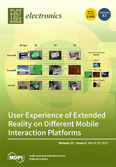
We evaluate the Extended Reality (XR) user experiences of multi-mode and multitasking among three mobile platforms: (1) bare smartphone (PhoneXR), (2) standalone mobile headset unit (ClosedXR), and (3) smartphone with clip-on lenses (LensXR). Results showed that users generally valued the immersive experience over usability—ClosedXR was clearly preferred over the others. Despite potentially offering a balanced level of immersion and usability with its touch-based interaction, LensXR was not generally received well. PhoneXR was not rated as particularly advantageous over ClosedXR even if it needed a controller. The usability suffered for ClosedXR only when the long text had to be entered. Thus, improving the 1D/2D operations in ClosedXR for operating and multitasking would be one way to weave XR into our lives with smartphones. View this paper
  • Issues are regarded as officially published after their release is announced to the table of contents alert mailing list.
  • You may sign up for e-mail alerts to receive table of contents of newly released issues.
  • PDF is the official format for papers published in both, html and pdf forms. To view the papers in pdf format, click on the "PDF Full-text" link, and use the free Adobe Reader to open them.
Order results
Result details
Section
Select all
Export citation of selected articles as:
18 pages, 1552 KiB  
Article
Enhancement of E-Learning Student’s Performance Based on Ensemble Techniques
by Abdulkream A. Alsulami, Abdullah S. AL-Malaise AL-Ghamdi and Mahmoud Ragab
Electronics 2023, 12(6), 1508; https://doi.org/10.3390/electronics12061508 - 22 Mar 2023
Cited by 12 | Viewed by 2314
Abstract
Educational institutions have dramatically increased in recent years, producing many graduates and postgraduates each year. One of the critical concerns of decision-makers is student performance. Educational data mining techniques are beneficial to explore uncovered data in data itself, creating a pattern to analyze [...] Read more.
Educational institutions have dramatically increased in recent years, producing many graduates and postgraduates each year. One of the critical concerns of decision-makers is student performance. Educational data mining techniques are beneficial to explore uncovered data in data itself, creating a pattern to analyze student performance. In this study, we investigate the student E-learning data that has increased significantly in the era of COVID-19. Thus, this study aims to analyze and predict student performance using information gathered from online systems. Evaluating the student E-learning data through the data mining model proposed in this study will help the decision-makers make informed and suitable decisions for their institution. The proposed model includes three traditional data mining methods, decision tree, Naive Bays, and random forest, which are further enhanced by the use of three ensemble techniques: bagging, boosting, and voting. The results demonstrated that the proposed model improved the accuracy from 0.75 to 0.77 when we used the DT method with boosting. Furthermore, the precision and recall results both improved from 0.76 to 0.78. Full article
(This article belongs to the Section Computer Science & Engineering)
Show Figures

Figure 1

Figure 1
<p>Student gender.</p>
Full article ">Figure 2
<p>Student nationalities.</p>
Full article ">Figure 3
<p>Student absences.</p>
Full article ">Figure 4
<p>Information gain filter.</p>
Full article ">Figure 5
<p>Correlation filter.</p>
Full article ">Figure 6
<p>Proposed model for predication of student’s performance.</p>
Full article ">Figure 7
<p>Traditional DM technique implementation using WEKA.</p>
Full article ">Figure 8
<p>Ensemble method (boosting) implementation using WEKA.</p>
Full article ">Figure 9
<p>Ensemble method (bagging) implementation using WEKA.</p>
Full article ">Figure 10
<p>The accuracy for traditional DM techniques.</p>
Full article ">Figure 11
<p>The accuracy of DM techniques and ensemble methods.</p>
Full article ">Figure 12
<p>Precision for DM techniques.</p>
Full article ">Figure 13
<p>The precision of DM and ensemble methods.</p>
Full article ">Figure 14
<p>Recall for DM techniques.</p>
Full article ">Figure 15
<p>The Recall of DM techniques and ensemble methods.</p>
Full article ">Figure 16
<p>F-measure for DM techniques.</p>
Full article ">Figure 17
<p>The F-measure of DM techniques and ensemble methods.</p>
Full article ">
16 pages, 6093 KiB  
Article
Near-Field Imaging of Dielectric Components Using an Array of Microwave Sensors
by Yuki Gao, Maryam Ravan and Reza K. Amineh
Electronics 2023, 12(6), 1507; https://doi.org/10.3390/electronics12061507 - 22 Mar 2023
Cited by 2 | Viewed by 2087
Abstract
Microwave imaging is a high-resolution, noninvasive, and noncontact method for detecting hidden defects, cracks, and objects with applications for testing nonmetallic components such as printed circuit boards, biomedical diagnosis, aerospace components inspection, etc. In this paper, an array of microwave sensors designed based [...] Read more.
Microwave imaging is a high-resolution, noninvasive, and noncontact method for detecting hidden defects, cracks, and objects with applications for testing nonmetallic components such as printed circuit boards, biomedical diagnosis, aerospace components inspection, etc. In this paper, an array of microwave sensors designed based on complementary split ring resonators (CSRR) are used to evaluate the hidden features in dielectric media with applications in nondestructive testing and biomedical diagnosis. In this array, each element resonates at a different frequency in the range of 1 GHz to 10 GHz. Even though the operating frequencies are not that high, the acquisition of evanescent waves in extreme proximity to the imaged object and processing them using near-field holographic imaging allows for obtaining high-resolution images. The performance of the proposed method is demonstrated through simulation and experimental results. Full article
(This article belongs to the Special Issue Applications of RF/Microwave/Millimeter-Wave/THz Imaging)
Show Figures

Figure 1

Figure 1
<p>Illustration of the near-field microwave holographic imaging setup.</p>
Full article ">Figure 2
<p>Microwave sensor array with (<b>a</b>) front surface and (<b>b</b>) back surface.</p>
Full article ">Figure 3
<p>Simulation setup in FEKO for the assessment of defects in dielectric materials.</p>
Full article ">Figure 4
<p>Reconstructed 1D images for defects with <math display="inline"><semantics> <mrow> <msub> <mi>W</mi> <mi>D</mi> </msub> </mrow> </semantics></math> = 2 mm, <math display="inline"><semantics> <mrow> <msub> <mi>H</mi> <mi>D</mi> </msub> </mrow> </semantics></math> = 2 mm, <math display="inline"><semantics> <mrow> <msub> <mi>H</mi> <mi>D</mi> </msub> </mrow> </semantics></math>= 4 mm, and <math display="inline"><semantics> <mrow> <msub> <mi>H</mi> <mi>D</mi> </msub> </mrow> </semantics></math> = 6 mm.</p>
Full article ">Figure 5
<p>Thickness estimation of defects with <math display="inline"><semantics> <mrow> <msub> <mi>H</mi> <mi>D</mi> </msub> </mrow> </semantics></math> of 2 mm, 4 mm, and 6 mm with (<b>a</b>) <math display="inline"><semantics> <mrow> <msub> <mi>W</mi> <mi>D</mi> </msub> </mrow> </semantics></math> = 2 mm, (<b>b</b>) <math display="inline"><semantics> <mrow> <msub> <mi>W</mi> <mi>D</mi> </msub> </mrow> </semantics></math> = 1 mm, and (<b>c</b>) <math display="inline"><semantics> <mrow> <msub> <mi>W</mi> <mi>D</mi> </msub> </mrow> </semantics></math> = 3 mm.</p>
Full article ">Figure 6
<p>Thickness estimation of defects with <math display="inline"><semantics> <mrow> <msub> <mi>H</mi> <mi>D</mi> </msub> </mrow> </semantics></math> of 2 mm, 4 mm, and 6 mm with <math display="inline"><semantics> <mrow> <msub> <mi>W</mi> <mi>D</mi> </msub> </mrow> </semantics></math> = 2 mm with a smaller sensor.</p>
Full article ">Figure 7
<p>Illustration of the simulation setup for skin tumor evaluation in FEKO.</p>
Full article ">Figure 8
<p>Illustration of the simulation setup for skin tumor evaluation in FEKO with: (<b>a</b>) <math display="inline"><semantics> <mrow> <msub> <mi>W</mi> <mrow> <mi>T</mi> <mn>1</mn> </mrow> </msub> <mo>=</mo> <mn>15</mn> <mrow> <mo> </mo> <mi>mm</mi> </mrow> </mrow> </semantics></math> and <math display="inline"><semantics> <mrow> <msub> <mi>H</mi> <mrow> <mi>T</mi> <mn>1</mn> </mrow> </msub> <mo>=</mo> <mn>1.5</mn> <mrow> <mo> </mo> <mi>mm</mi> </mrow> </mrow> </semantics></math>, (<b>b</b>) <math display="inline"><semantics> <mrow> <msub> <mi>W</mi> <mrow> <mi>T</mi> <mn>1</mn> </mrow> </msub> <mo>=</mo> <mn>15</mn> <mrow> <mo> </mo> <mi>mm</mi> </mrow> </mrow> </semantics></math>, <math display="inline"><semantics> <mrow> <msub> <mi>H</mi> <mrow> <mi>T</mi> <mn>1</mn> </mrow> </msub> <mo>=</mo> <mn>1.5</mn> <mrow> <mo> </mo> <mi>mm</mi> </mrow> </mrow> </semantics></math>, <math display="inline"><semantics> <mrow> <msub> <mi>W</mi> <mrow> <mi>T</mi> <mn>2</mn> </mrow> </msub> <mo>=</mo> <mn>10</mn> <mrow> <mo> </mo> <mi>mm</mi> </mrow> </mrow> </semantics></math>, and <math display="inline"><semantics> <mrow> <msub> <mi>H</mi> <mrow> <mi>T</mi> <mn>2</mn> </mrow> </msub> <mo>=</mo> <mn>3</mn> <mrow> <mo> </mo> <mi>mm</mi> </mrow> </mrow> </semantics></math>, and (<b>c</b>) <math display="inline"><semantics> <mrow> <msub> <mi>W</mi> <mrow> <mi>T</mi> <mn>1</mn> </mrow> </msub> <mo>=</mo> <mn>15</mn> <mrow> <mo> </mo> <mi>mm</mi> </mrow> <mo>,</mo> <mo> </mo> <msub> <mi>H</mi> <mrow> <mi>T</mi> <mn>1</mn> </mrow> </msub> <mo>=</mo> <mn>1.5</mn> <mrow> <mo> </mo> <mi>mm</mi> </mrow> <mo>,</mo> <mo> </mo> <msub> <mi>W</mi> <mrow> <mi>T</mi> <mn>2</mn> </mrow> </msub> <mo>=</mo> <mn>10</mn> <mrow> <mo> </mo> <mi>mm</mi> </mrow> <mo>,</mo> <mo> </mo> <msub> <mi>H</mi> <mrow> <mi>T</mi> <mn>2</mn> </mrow> </msub> <mo>=</mo> <mn>3</mn> <mrow> <mo> </mo> <mi>mm</mi> </mrow> <mo>,</mo> </mrow> </semantics></math> <math display="inline"><semantics> <mrow> <msub> <mi>W</mi> <mrow> <mi>T</mi> <mn>3</mn> </mrow> </msub> <mo>=</mo> <mn>5</mn> <mrow> <mo> </mo> <mi>mm</mi> </mrow> </mrow> </semantics></math>, and <math display="inline"><semantics> <mrow> <msub> <mi>H</mi> <mrow> <mi>T</mi> <mn>3</mn> </mrow> </msub> <mo>=</mo> <mn>4.5</mn> <mrow> <mo> </mo> <mi>mm</mi> </mrow> </mrow> </semantics></math>.</p>
Full article ">Figure 9
<p>Depth estimation of the tumor for actual thicknesses of 1.5 mm, 3 mm, and 4.5 mm.</p>
Full article ">Figure 10
<p>Main components of the microwave imaging system with: (<b>a</b>) wood with defects as MUT, (<b>b</b>) a pile of paper with copper strips as MUT, (<b>c</b>) front view of the multifrequency near-field sensor, and (<b>d</b>) back view of the multifrequency near-field sensor.</p>
Full article ">Figure 11
<p>Simulated and measured <math display="inline"><semantics> <mrow> <mrow> <mo>|</mo> <mrow> <msub> <mi mathvariant="normal">S</mi> <mrow> <mn>21</mn> </mrow> </msub> </mrow> <mo>|</mo> </mrow> </mrow> </semantics></math> data without the presence of object.</p>
Full article ">Figure 12
<p>Reconstructed 1D images of defect with a depth of 4 mm when using 5 and 6 frequencies.</p>
Full article ">Figure 13
<p>Thickness estimation of defects with a depth of 4 mm using data at 5 and 6 resonant frequencies.</p>
Full article ">Figure 14
<p>Reconstructed 1D images for copper strips placed at a depth of 1 mm when using data at 5 and 6 resonant frequencies.</p>
Full article ">Figure 15
<p>Reconstructed 1D images for copper strips placed at a depth of 5 mm when using data at 5 and 6 resonant frequencies.</p>
Full article ">Figure 16
<p>Reconstructed 1D images for copper strips placed at a depth of 13 mm when using data at 5 and 6 frequencies.</p>
Full article ">
17 pages, 13570 KiB  
Review
Review on Key Technologies and Development of Magnetic Coupling Resonant-Dynamic Wireless Power Transfer for Unmanned Ground Vehicles
by Feifan Xu, Shuguang Wei, Dong Yuan and Jiaqi Li
Electronics 2023, 12(6), 1506; https://doi.org/10.3390/electronics12061506 - 22 Mar 2023
Cited by 4 | Viewed by 1553
Abstract
With the fast development of magnetic coupling resonant-dynamic wireless power transfer (MCR-DWPT), it is more likely that high-efficiency wireless charging between unmanned ground vehicles (UGVs) will be practically realized, especially in desolate places that are far away from a city center or charging [...] Read more.
With the fast development of magnetic coupling resonant-dynamic wireless power transfer (MCR-DWPT), it is more likely that high-efficiency wireless charging between unmanned ground vehicles (UGVs) will be practically realized, especially in desolate places that are far away from a city center or charging depot and always experiencing large load fluctuations, varying operating conditions, and complex working targets. Based on this, the wireless charging of UGVs demands higher reliability and efficiency. This paper reviews the MCR-DWPT system of UGVs, and the basic structure and key technologies are introduced. Then, the key technologies, which include the coupling device design, compensation topology design, and system control strategy, are discussed in detail. After that, by considering the current research, the main challenges of the MCR-DWPT of UGVs are investigated and its developing prospects are explored. Full article
(This article belongs to the Topic Advanced Wireless Charging Technology)
Show Figures

Figure 1

Figure 1
<p>General structure of MCR-DWPT of UGVs.</p>
Full article ">Figure 2
<p>Spatial motion modes of coupling devices: (<b>a</b>) reference state; (<b>b</b>) axial offset; (<b>c</b>) horizontal offset; (<b>d</b>) horizontal turnover; (<b>e</b>) horizontal rotation along the symmetry axis.</p>
Full article ">Figure 3
<p>Four coupling device structures of the receiver prototype model: (<b>a</b>) CP; (<b>b</b>) DDP; (<b>c</b>) BBP; and (<b>d</b>) DDQP.</p>
Full article ">Figure 4
<p>Prototype of the coupling device with mechanical structure.</p>
Full article ">Figure 5
<p>Four basic compensation topologies: (<b>a</b>) S/S; (<b>b</b>) S/P; (<b>c</b>) P/S; and (<b>d</b>) P/P.</p>
Full article ">Figure 6
<p>High-order compensation topologies: (<b>a</b>) LCL/LCL; (<b>b</b>) LCC/LCC; (<b>c</b>) LC/S; (<b>d</b>) LCC/S; and (<b>e</b>) S/LCC.</p>
Full article ">Figure 7
<p>The structures of the three reconfigurable compensation circuits: (<b>a</b>) a reconfigurable compensation circuit topology based on the receiver of the LCL-type compensation topology; (<b>b</b>) a reconfigurable compensation circuit topology based on the equivalent detuning S/S-type compensation topology; and (<b>c</b>) a reconfigurable compensation circuit topology based on a capacitance matrix (capacitance matrix section).</p>
Full article ">Figure 8
<p>Control structures of MCR-DWPT of UGVs.</p>
Full article ">
16 pages, 5072 KiB  
Article
HTC-Grasp: A Hybrid Transformer-CNN Architecture for Robotic Grasp Detection
by Qiang Zhang, Jianwei Zhu, Xueying Sun and Mingmin Liu
Electronics 2023, 12(6), 1505; https://doi.org/10.3390/electronics12061505 - 22 Mar 2023
Cited by 3 | Viewed by 2217
Abstract
Accurately detecting suitable grasp areas for unknown objects through visual information remains a challenging task. Drawing inspiration from the success of the Vision Transformer in vision detection, the hybrid Transformer-CNN architecture for robotic grasp detection, known as HTC-Grasp, is developed to improve the [...] Read more.
Accurately detecting suitable grasp areas for unknown objects through visual information remains a challenging task. Drawing inspiration from the success of the Vision Transformer in vision detection, the hybrid Transformer-CNN architecture for robotic grasp detection, known as HTC-Grasp, is developed to improve the accuracy of grasping unknown objects. The architecture employs an external attention-based hierarchical Transformer as an encoder to effectively capture global context and correlation features across the entire dataset. Furthermore, a channel-wise attention-based CNN decoder is presented to adaptively adjust the weight of the channels in the approach, resulting in more efficient feature aggregation. The proposed method is validated on the Cornell and the Jacquard dataset, achieving an image-wise detection accuracy of 98.3% and 95.8% on each dataset, respectively. Additionally, the object-wise detection accuracy of 96.9% and 92.4% on the same datasets are achieved based on this method. A physical experiment is also performed using the Elite 6Dof robot, with a grasping accuracy rate of 93.3%, demonstrating the proposed method’s ability to grasp unknown objects in real scenarios. The results of this study indicate that the proposed method outperforms other state-of-the-art methods. Full article
(This article belongs to the Special Issue Recent Advances in Industrial Robots)
Show Figures

Figure 1

Figure 1
<p>Overview of HTC-Grasp. <span class="html-italic">H</span> and <span class="html-italic">W</span> in the figure correspond to the height and width of the feature map. <math display="inline"><semantics> <mrow> <msub> <mrow> <mi>C</mi> </mrow> <mrow> <mi>i</mi> </mrow> </msub> </mrow> </semantics></math> is the channel size of the feature map.</p>
Full article ">Figure 2
<p>The architecture of external attention block.</p>
Full article ">Figure 3
<p>Res-Channel attention block.</p>
Full article ">Figure 4
<p>Comparison of predicted heatmaps on Cornell Dataset. The first and second columns depict RGB and depth images, respectively. The third column displays the grasping rectangles and successful grasps are marked as rectangles. The final three columns depict heatmaps indicating the quality, angle, and width of the detected grasps. The quality heatmaps characterizes the degree of confidence that each pixel is a valid grasping location.</p>
Full article ">Figure 5
<p>Comparison of predicted heatmaps on Jacquard Dataset. The first and second columns depict RGB and depth images, respectively. The third column displays the grasping rectangles and successful grasps are marked as rectangles. The final three columns depict heatmaps indicating the quality, angle, and width of the detected grasps. The quality heatmaps characterizes the degree of confidence that each pixel is a valid grasping location.</p>
Full article ">Figure 6
<p>The test result of HTC-Grasp in the real-world multiple objects environment. The first and second columns depict RGB and depth images, respectively. The third column displays the grasping rectangles and successful grasps are marked as rectangles. The final three columns depict heatmaps indicating the quality, angle, and width of the detected grasps. The quality heatmaps characterizes the degree of confidence that each pixel is a valid grasping location.</p>
Full article ">Figure 7
<p>Realistic scenario experiment setup. The experimental equipment includes the Elite EC-66 robot, the Fin Ray effect-inspired soft parallel gripper and the Orbbec Femto-W RGB-D camera.</p>
Full article ">Figure 8
<p>Household objects used in the experiment.</p>
Full article ">Figure 9
<p>Example of the robotic grasp process. (<b>a</b>) shows the initial state of the robot. (<b>b</b>) illustrates the robot’s gripper has moved to the target to be grasped. (<b>c</b>) shows the state of the object being grasped. (<b>d</b>) demonstrates the target being moved to another location.</p>
Full article ">
17 pages, 817 KiB  
Article
Query Join Order Optimization Method Based on Dynamic Double Deep Q-Network
by Lixia Ji, Runzhe Zhao, Yiping Dang, Junxiu Liu and Han Zhang
Electronics 2023, 12(6), 1504; https://doi.org/10.3390/electronics12061504 - 22 Mar 2023
Cited by 1 | Viewed by 2055
Abstract
A join order directly affects database query performance and computational overhead. Deep reinforcement learning (DRL) can explore efficient query plans while not exhausting the search space. However, the deep Q network (DQN) suffers from the overestimation of action values in query optimization, which [...] Read more.
A join order directly affects database query performance and computational overhead. Deep reinforcement learning (DRL) can explore efficient query plans while not exhausting the search space. However, the deep Q network (DQN) suffers from the overestimation of action values in query optimization, which can lead to limited query performance. In addition, ε-greedy exploration is not efficient enough and does not enable deep exploration. Accordingly, in this paper, we propose a dynamic double DQN (DDQN) order selection method(DDOS) for join order optimization. First, the method models the join query as a Markov decision process (MDP), then solves the DRL model by integrating the network model DQN and DDQN weighting into the DRL model’s estimation error problem in query joining, and finally improves the quality of developing query plans. And actions are selected using a dynamic progressive search strategy to improve the randomness and depth of exploration and accumulate a high information gain of exploration. The performance of the proposed method is compared with those of dynamic programming, heuristic algorithms, and DRL optimization methods based on the query set Join Order Benchmark (JOB). The experimental results show that the proposed method can effectively improve the query performance with a favorable generalization ability and robustness, and outperforms other baselines in multi-join query applications. Full article
(This article belongs to the Special Issue Advanced Techniques in Computing and Security)
Show Figures

Figure 1

Figure 1
<p>Order of joins regarding the three table relations. (C(R<math display="inline"><semantics> <msub> <mrow/> <mi>i</mi> </msub> </semantics></math>) denotes the cost of coming to access the basic relation R<math display="inline"><semantics> <msub> <mrow/> <mi>i</mi> </msub> </semantics></math>, and C(R<math display="inline"><semantics> <msub> <mrow/> <mi>i</mi> </msub> </semantics></math>,R<math display="inline"><semantics> <mrow> <msub> <mrow/> <mi>i</mi> </msub> <mo>+</mo> <mn>1</mn> </mrow> </semantics></math>) denotes the cost of R<math display="inline"><semantics> <msub> <mrow/> <mi>i</mi> </msub> </semantics></math> and R<math display="inline"><semantics> <mrow> <msub> <mrow/> <mi>i</mi> </msub> <mo>+</mo> <mn>1</mn> </mrow> </semantics></math> joins).</p>
Full article ">Figure 2
<p>Workflow for developing a query plan. (The most important part is to adjust the network parameters through DDOS training to obtain the connection plan with the minimum cost and the shortest execution time. Where (<span class="html-italic">s</span>, <span class="html-italic">a</span>, <span class="html-italic">r</span>, <math display="inline"><semantics> <msup> <mi>s</mi> <mo>′</mo> </msup> </semantics></math>) represents the reward <span class="html-italic">r</span> and the next state <span class="html-italic">s</span><math display="inline"><semantics> <msup> <mrow/> <mo>′</mo> </msup> </semantics></math> obtained by taking action <span class="html-italic">a</span> in state <span class="html-italic">s</span>).</p>
Full article ">Figure 3
<p>Action vector representation process.</p>
Full article ">Figure 4
<p>Architecture of the query cost prediction model (input to the network after obtaining the SQL vector, join on the query plan tree, and output of the long-term plan cost at a fully connected layer after network training).</p>
Full article ">Figure 5
<p>Comparison of the average reward value of DDQN and DDOS under different parameters (higher average reward value means a smaller and more reasonable query join cost).</p>
Full article ">Figure 6
<p>Comparison of the query plan delay times for different optimization methods.</p>
Full article ">Figure 7
<p>Comparison of the mean relative cost (in log scale) of DDOS, Rejoin and DQ.</p>
Full article ">Figure 8
<p>Relative execution cost of the DDOS, DDQN, DQ, Rejoin, and QuickPick-1000 queries.</p>
Full article ">
16 pages, 7425 KiB  
Article
A Broadband Analog Predistortion Linearizer Based on GaAs MMIC for Ka-Band TWTAs
by Ting Liu, Xiaobao Su, Gang Wang, Bin Zhao, Rui Fu and Dan Zhu
Electronics 2023, 12(6), 1503; https://doi.org/10.3390/electronics12061503 - 22 Mar 2023
Cited by 2 | Viewed by 1880
Abstract
In this article, a Ka-band broadband analog predistortion (APD) microwave monolithic integrated circuit (MMIC) with independent tunability based on a 0.15 μm GaAs pHEMT process is proposed, which can be cascaded in front of traveling wave tube amplifiers (TWTAs) to improve their linearity. [...] Read more.
In this article, a Ka-band broadband analog predistortion (APD) microwave monolithic integrated circuit (MMIC) with independent tunability based on a 0.15 μm GaAs pHEMT process is proposed, which can be cascaded in front of traveling wave tube amplifiers (TWTAs) to improve their linearity. The influence of different diode sizes on the parameters of Schottky diodes is analyzed and used to design the gain and phase nonlinear branches. The broadband APD MMIC is realized based on a dual-branch vector synthesis design and nonlinear frequency adjust module (NFAM). The independent tunability and broadband characteristics of the APD MMIC are verified by simulated and measured results with an error of less than 5%. Furthermore, a Ka-band 60 W TWTA is linearized by the APD MMIC, and the gain and phase compressions are reduced from 8 dB and 50° to within 3 dB and 12°, respectively. The third-order intermodulation (C/IM3) is greater than 28 dBc and noise power ratio (NPR) is greater than 15.7 dBc at 3 dB output power backoff (OPBO) over the operating band of 25.1~27.5 GHz, indicating that the APD MMIC can improve the nonlinearity of TWTA effectively under broadband signals. Full article
(This article belongs to the Special Issue RF/Microwave Circuits for 5G and Beyond, Volume II)
Show Figures

Figure 1

Figure 1
<p>Analog predistortion MMIC schematic.</p>
Full article ">Figure 2
<p>(<b>a</b>) The GaAs pHEMT diode layout; (<b>b</b>) the GaAs pHEMT diode model.</p>
Full article ">Figure 3
<p><span class="html-italic">I-V</span> curve for different sizes of GaAs pHEMT Schottky diodes.</p>
Full article ">Figure 4
<p>Schematic diagram of (<b>a</b>) gain expansion and (<b>b</b>) phase expansion independently tuning.</p>
Full article ">Figure 5
<p>Simulated results of the independent tuning of (<b>a</b>) gain conversion and (<b>b</b>) phase conversion.</p>
Full article ">Figure 6
<p>(<b>a</b>) Phase expansion difference with Cj. (<b>b</b>) Gain and phase expansion after adding NFAM to APD MMIC.</p>
Full article ">Figure 7
<p>APD MMIC Photo.</p>
Full article ">Figure 8
<p>The test platform for APD MMIC and TWTA cascade with proposed APD MMIC.</p>
Full article ">Figure 9
<p>Measured results of (<b>a</b>) gain and phase expansion and (<b>b</b>) gain under saturation and small signal.</p>
Full article ">Figure 10
<p>Measured results of independent tuning of (<b>a</b>) gain conversion and (<b>b</b>) phase conversion.</p>
Full article ">Figure 11
<p>TWTA gain and phase conversion before and after the proposed APD MMIC circuit.</p>
Full article ">Figure 12
<p>The C/IM3 performance before and after the proposed APD MMIC circuit.</p>
Full article ">Figure 13
<p>NPR performance of LTWTA with a signal width change when OBO = 3 dB.</p>
Full article ">
14 pages, 4746 KiB  
Article
Long-Distance Person Detection Based on YOLOv7
by Fan Tang, Fang Yang and Xianqing Tian
Electronics 2023, 12(6), 1502; https://doi.org/10.3390/electronics12061502 - 22 Mar 2023
Cited by 14 | Viewed by 6738
Abstract
In the research field of small object detection, most object detectors have been successfully used for pedestrian detection, face recognition, lost and found, and automatic driving, among other applications, and have achieved good results. However, when general object detectors encounter challenging low-resolution images [...] Read more.
In the research field of small object detection, most object detectors have been successfully used for pedestrian detection, face recognition, lost and found, and automatic driving, among other applications, and have achieved good results. However, when general object detectors encounter challenging low-resolution images from the TinyPerson dataset, they will produce undesirable detection results because of the dense occlusion between people and different body poses. In order to solve these problems, this paper proposes a tiny object detection method TOD-YOLOv7 based on YOLOv7.First, this paper presents a reconstruction of the YOLOv7 network by adding a tiny object detection layer to enhance its detection ability. Then, we use the recursive gated convolution module to realize the interaction with the higher-order space to accelerate the model initialization process and reduce the reasoning time. Secondly, this paper proposes the integration of a coordinate attention mechanism into the YOLOv7 feature extraction network to strengthen the pedestrian object information and weaken the background information.Additionally, we leverage data augmentation techniques to improve the representation learning of the algorithm. The results show that compared with the baseline model YOLOv7, the detection accuracy of this model on the TinyPerson dataset is improved from 7.1% to 9.5%, and the detection speed reaches 208 frames per second (FPS). The algorithm of this paper is shown to achieve better detection results for tiny object detection. Full article
Show Figures

Figure 1

Figure 1
<p>Intuitive examples on TinyPerson dataset [<a href="#B2-electronics-12-01502" class="html-bibr">2</a>] demonstrate the differences before and after the algorithmic improvements. (<b>a</b>) In the original YOLOv7 detection, many objects are missed in the enlarged detail. (<b>b</b>) This paper’s improved algorithm TOD-YOLOv7 can detect more objects.</p>
Full article ">Figure 2
<p>Results of different data augmentation methods.</p>
Full article ">Figure 3
<p>The network structure of TOD-YOLOv7. The red dotted box in the figure represents the extra detection head that this paper added to the model. The lower part of the figure illustrates the structural schematic diagram of specific components.</p>
Full article ">Figure 4
<p><math display="inline"><semantics> <mrow> <msup> <mi>g</mi> <mi>n</mi> </msup> <mi>C</mi> <mi>o</mi> <mi>n</mi> <mi>v</mi> </mrow> </semantics></math> module realizes spatial information interaction of any stage. (<b>a</b>) Object key feature (area A) and adjacent feature (area B). (<b>b</b>) Three-order information interaction is realized through element multiplication and recursive operation between the target research area and adjacent features.</p>
Full article ">Figure 5
<p>Network structure of coordinate attention mechanism.</p>
Full article ">Figure 6
<p>CA focuses on key information by participating in the calculation in MP module.</p>
Full article ">Figure 7
<p>Training curve of TOD-YOLOv7 model. (<b>a</b>) is the curve of precision. (<b>b</b>) is the curve of recall. (<b>c</b>) is the curve of AP@50. (<b>d</b>) is the curve of AP@50:5:95.</p>
Full article ">
13 pages, 10219 KiB  
Article
Robust Graph Neural-Network-Based Encoder for Node and Edge Deep Anomaly Detection on Attributed Networks
by G. Victor Daniel, Kandasamy Chandrasekaran, Venkatesan Meenakshi and Prabhavathy Paneer
Electronics 2023, 12(6), 1501; https://doi.org/10.3390/electronics12061501 - 22 Mar 2023
Cited by 3 | Viewed by 2371
Abstract
The task of identifying anomalous users on attributed social networks requires the detection of users whose profile attributes and network structure significantly differ from those of the majority of the reference profiles. GNN-based models are well-suited for addressing the challenge of integrating network [...] Read more.
The task of identifying anomalous users on attributed social networks requires the detection of users whose profile attributes and network structure significantly differ from those of the majority of the reference profiles. GNN-based models are well-suited for addressing the challenge of integrating network structure and node attributes into the learning process because they can efficiently incorporate demographic data, activity patterns, and other relevant information. Aggregate operations, such as sum or mean pooling, are utilized by Graph Neural Networks (GNNs) to combine the representations of neighboring nodes within a graph. However, these aggregate operations can cause problems in detecting anomalous nodes. There are two main issues to consider when utilizing aggregate operations in GNNs. Firstly, the presence of anomalous neighboring nodes may affect the representation of normal nodes, leading to false positives. Secondly, anomalous nodes may be overlooked as their representation is flattened during the aggregate operation, leading to false negatives. The proposed approach, AnomEn, is a robust graph neural network developed for anomaly detection. It addresses the challenges of false positives and false negatives using a weighted aggregate mechanism. This mechanism is designed to differentiate between a node’s own features and the features of its neighbors by placing greater emphasis on a node’s own features and less emphasis on its neighbors’ features. The system can preserve the node’s original characteristics, whether the node is normal or anomalous. This work proposes not only a robust graph neural network, namely, AnomEn, but also specific anomaly detection structures for nodes and edges. The proposed AnomEn method serves as the encoder in the node and edge anomaly detection architectures and was tested on multiple datasets. Experiments were conducted to validate the effectiveness of the proposed method as a graph neural network encoder. The findings demonstrated the robustness of the proposed method in detecting anomalies. The proposed method outperforms other existing methods in node anomaly detection tasks by 5.63% and edge anomaly detection tasks by 7.87%. Full article
Show Figures

Figure 1

Figure 1
<p>The Proposed Framework for Node Anomaly Detection (NodeAnomEn) in Attributed Networks.</p>
Full article ">Figure 2
<p>The Proposed Framework (EdgeAnomEn) for Edge Anomaly Detection in Attributed Networks.</p>
Full article ">Figure 3
<p>NodeAnomEn vs. DOMINANT.</p>
Full article ">Figure 4
<p>NodeAnomEn vs. DOMINANT.</p>
Full article ">Figure 5
<p>Comparison of base methods and proposed method EdgeAnomEn in terms of accuracy and AUC for edge anomaly detection on PolitiFact and GossipCop datasets. The figure displays the performance trend of the different methods, with higher values indicating better performance.</p>
Full article ">
15 pages, 8952 KiB  
Article
State Parameter Estimation of Intelligent Vehicles Based on an Adaptive Unscented Kalman Filter
by Yu Wang, Yushan Li and Ziliang Zhao
Electronics 2023, 12(6), 1500; https://doi.org/10.3390/electronics12061500 - 22 Mar 2023
Cited by 7 | Viewed by 1909
Abstract
The premise of vehicle intelligent decision making is to obtain vehicle motion state parameters accurately and in real-time. Several state parameters cannot be measured directly by vehicle sensors, so estimation algorithms based on filtering are effective solutions. The most representative algorithm is the [...] Read more.
The premise of vehicle intelligent decision making is to obtain vehicle motion state parameters accurately and in real-time. Several state parameters cannot be measured directly by vehicle sensors, so estimation algorithms based on filtering are effective solutions. The most representative algorithm is the Kalman filter, especially the standard unscented Kalman filter (UKF) that has been widely used in vehicle state estimation because of its superiority in dealing with nonlinear filtering problems. However, although the UKF assumes that the noise statistics of the system are known, due to the complex and changeable operating conditions, sensor aging and other factors, these noises vary. In order to realize high-precision vehicle state estimation, a noise-adaptive UKF algorithm is proposed in this article. The maximum a posteriori (MAP) algorithm is used to dynamically update the noise of the vehicle system, and it is embedded into the update step of the UKF to form an adaptive unscented Kalman filter (AUKF). The system will dynamically update the noise when noise statistics are unknown and prevent filter divergence by adjusting the mean and covariance of the estimated noise to improve accuracy. On this basis, the proposed method is verified by the joint simulation of CarSim and Matlab/Simulink, confirming that the AUKF performs better than the standard UKF in estimation accuracy and stability under different degrees of noise disturbance, and the estimation accuracy for the yaw rate, side slip angle and longitudinal velocity is improved by 20.08%, 40.98% and 89.91%, respectively. Full article
(This article belongs to the Special Issue Feature Papers in Electrical and Autonomous Vehicles)
Show Figures

Figure 1

Figure 1
<p>3-DOF vehicle model.</p>
Full article ">Figure 2
<p>The framework of the AUKF algorithm.</p>
Full article ">Figure 3
<p>Simulation results of yaw rate. (<b>a</b>) Comparison of estimated results and (<b>b</b>) comparison of estimated error.</p>
Full article ">Figure 4
<p>Simulation results of side slip angle. (<b>a</b>) Comparison of estimated results and (<b>b</b>) comparison of estimated error.</p>
Full article ">Figure 5
<p>Simulation results of longitudinal velocity. (<b>a</b>) Comparison of estimated results and (<b>b</b>) comparison of estimated error.</p>
Full article ">Figure 6
<p>Simulation results of yaw rate. (<b>a</b>) Comparison of estimated results and (<b>b</b>) comparison of estimated error.</p>
Full article ">Figure 7
<p>Simulation results of side slip angle. (<b>a</b>) Comparison of estimated results and (<b>b</b>) comparison of estimated error.</p>
Full article ">Figure 8
<p>Simulation results of longitudinal velocity. (<b>a</b>) Comparison of estimated results and (<b>b</b>) comparison of estimated error.</p>
Full article ">Figure 9
<p>Simulation results of yaw rate. (<b>a</b>) Comparison of estimated results and (<b>b</b>) comparison of estimated error.</p>
Full article ">Figure 10
<p>Simulation results of side slip angle. (<b>a</b>) Comparison of estimated results and (<b>b</b>) comparison of estimated error.</p>
Full article ">Figure 11
<p>Simulation results of longitudinal velocity. (<b>a</b>) Comparison of estimated results and (<b>b</b>) comparison of estimated error.</p>
Full article ">Figure 12
<p>Simulation results of yaw rate. (<b>a</b>) Comparison of estimated results and (<b>b</b>) comparison of estimated error.</p>
Full article ">Figure 13
<p>Simulation results of side slip angle. (<b>a</b>) Comparison of estimated results and (<b>b</b>) comparison of estimated error.</p>
Full article ">Figure 14
<p>Simulation results of longitudinal velocity. (<b>a</b>) Comparison of estimated results and (<b>b</b>) comparison of estimated error.</p>
Full article ">
14 pages, 2877 KiB  
Article
AoI-Bounded Scheduling for Industrial Wireless Sensor Networks
by Chenggen Pu, Han Yang, Ping Wang and Changjie Dong
Electronics 2023, 12(6), 1499; https://doi.org/10.3390/electronics12061499 - 22 Mar 2023
Cited by 2 | Viewed by 1740
Abstract
Age of information (AoI) is an emerging network metric that measures information freshness from an application layer perspective. It can evaluate the timeliness of information in industrial wireless sensor networks (IWSNs). Previous research has primarily focused on minimizing the long-term average AoI of [...] Read more.
Age of information (AoI) is an emerging network metric that measures information freshness from an application layer perspective. It can evaluate the timeliness of information in industrial wireless sensor networks (IWSNs). Previous research has primarily focused on minimizing the long-term average AoI of the entire system. However, in practical industrial applications, optimizing the average AoI does not guarantee that the peak AoI of each data packet is within a bounded interval. If the AoI of certain packets exceeds the predetermined threshold, it can have a significant impact on the stability of the industrial control system. Therefore, this paper studies the scheduling problem subject to a hard AoI performance requirement in IWSNs. First, we propose a low-complexity AoI-bounded scheduling algorithm for IWSNs that guarantees that the AoI of each packet is within a bounded interval. Then, we analyze the schedulability conditions of the algorithm and propose a method to decrease the peak AoI of nodes with higher AoI requirements. Finally, we present a numerical example that illustrates the proposed algorithm step by step. The results demonstrate the effectiveness of our algorithm, which can guarantee bounded AoI intervals (BAIs) for all nodes. Full article
Show Figures

Figure 1

Figure 1
<p>Evolution of node’s AoI with respect to different transmission intervals. (<bold>a</bold>) The change of node’s AoI when <inline-formula><mml:math id="mm184"><mml:semantics><mml:mrow><mml:msub><mml:mi>I</mml:mi><mml:mi>i</mml:mi></mml:msub><mml:mo>&gt;</mml:mo><mml:msub><mml:mi>T</mml:mi><mml:mi>i</mml:mi></mml:msub></mml:mrow></mml:semantics></mml:math></inline-formula>; (<bold>b</bold>) the change of node’s AoI when <inline-formula><mml:math id="mm185"><mml:semantics><mml:mrow><mml:msub><mml:mi>I</mml:mi><mml:mi>i</mml:mi></mml:msub><mml:mo>=</mml:mo><mml:msub><mml:mi>T</mml:mi><mml:mi>i</mml:mi></mml:msub></mml:mrow></mml:semantics></mml:math></inline-formula> under ideal conditions; (<bold>c</bold>) the change of node’s AoI when <inline-formula><mml:math id="mm186"><mml:semantics><mml:mrow><mml:mfrac><mml:mrow><mml:msub><mml:mi>T</mml:mi><mml:mi>i</mml:mi></mml:msub></mml:mrow><mml:mn>2</mml:mn></mml:mfrac><mml:mo>&lt;</mml:mo><mml:msub><mml:mi>I</mml:mi><mml:mi>i</mml:mi></mml:msub><mml:mo>&lt;</mml:mo><mml:msub><mml:mi>T</mml:mi><mml:mi>i</mml:mi></mml:msub></mml:mrow></mml:semantics></mml:math></inline-formula>; (<bold>d</bold>) the change of node’s AoI when <inline-formula><mml:math id="mm187"><mml:semantics><mml:mrow><mml:msub><mml:mi>I</mml:mi><mml:mi>i</mml:mi></mml:msub><mml:mo>&lt;</mml:mo><mml:mfrac><mml:mrow><mml:msub><mml:mi>T</mml:mi><mml:mi>i</mml:mi></mml:msub></mml:mrow><mml:mn>2</mml:mn></mml:mfrac></mml:mrow></mml:semantics></mml:math></inline-formula>.</p>
Full article ">Figure 2
<p>The superframe is divided into multiple minimum transmission units, where the length of each transmission unit is equal to the minimum sampling period in all nodes, and <inline-formula><mml:math id="mm188"><mml:semantics><mml:mi>σ</mml:mi></mml:semantics></mml:math></inline-formula> time slots are reserved for aperiodic data at the end of each transmission unit.</p>
Full article ">Figure 3
<p>Illustration of the time slot allocation.</p>
Full article ">Figure 4
<p>The real-time AoI, with the corresponding peak AoI and benchmark of three sample nodes: (<bold>a</bold>) node #2, (<bold>b</bold>) node #6, (<bold>c</bold>) node #9.</p>
Full article ">Figure 5
<p>Boxplot of AoI for all ten sensor nodes.</p>
Full article ">Figure 6
<p>The AoI of node #9 with different <inline-formula><mml:math id="mm189"><mml:semantics><mml:mrow><mml:msub><mml:mi>α</mml:mi><mml:mn>9</mml:mn></mml:msub></mml:mrow></mml:semantics></mml:math></inline-formula>.</p>
Full article ">Figure 7
<p>Boxplot of AoI for node #9 with different TIC <inline-formula><mml:math id="mm190"><mml:semantics><mml:mrow><mml:msub><mml:mi>α</mml:mi><mml:mn>9</mml:mn></mml:msub></mml:mrow></mml:semantics></mml:math></inline-formula>.</p>
Full article ">Figure 8
<p>Schedulability analysis with respect to varying numbers of nodes and sampling periods.</p>
Full article ">
13 pages, 1586 KiB  
Article
A Real-Time, Open-Source, IoT-like, Wearable Monitoring Platform
by Andrea Baldini, Roberto Garofalo, Enzo Pasquale Scilingo and Alberto Greco
Electronics 2023, 12(6), 1498; https://doi.org/10.3390/electronics12061498 - 22 Mar 2023
Cited by 6 | Viewed by 2701
Abstract
The spread of informatics and electronic systems capable of the real-time monitoring of multiple psychophysiological signals has continuously grown in the last few years. In this study, we propose a novel open-source wearable monitoring platform (WMP) to synchronously acquire and process multiple physiological [...] Read more.
The spread of informatics and electronic systems capable of the real-time monitoring of multiple psychophysiological signals has continuously grown in the last few years. In this study, we propose a novel open-source wearable monitoring platform (WMP) to synchronously acquire and process multiple physiological signals in a real-time fashion. Specifically, we developed an IoT-like modular and fully open-source platform composed of two main blocks that on the one hand connect multiple devices (the sensor fusion unit) and on the other hand process and store the sensors’ data through the internet (the remote storing and processing unit). To test the proposed platform and its computational performance, 15 subjects underwent an experimental protocol, in which they were exposed to rest and stressful sessions implementing the Stroop Color and Word Test (SCWT). Statistical analysis was performed to verify whether the WMP could monitor the expected variations in the subjects’ psychophysiological state induced by the SCWT. The WMP showed very good computational performance for data streaming, remote storing, and real-time processing. Moreover, the experimental results showed that the platform was reliable when capturing physiological changes coherently with the emotional salience of the SCWT. Full article
(This article belongs to the Special Issue Digital Twin Technology: New Frontiers for Personalized Healthcare)
Show Figures

Figure 1

Figure 1
<p>Summary of the WMP architecture. On the left side: The sensor fusion unit (SFU). On the right side: The remote data storage and processing unit (RDSPU).</p>
Full article ">Figure 2
<p>The sensor fusion unit (SFU). On the left: The sensor layer is composed of the wearable devices to be connected. SP1, SP2, and SP3 represent the dedicated acquiring subprocesses for the streaming devices. SP4 is the subprocess in charge of data gathering and streaming over the MQTT protocol. On the right: The PyQt6 user interface developed to handle the data acquisition from the Shimmer3 GSR+ unit and DSI-24 system alongside metadata and subjects’ personal information.</p>
Full article ">Figure 3
<p>(<b>a</b>) The DSI-24 system. (<b>b</b>) The Shimmer3 GSR+ unit.</p>
Full article ">Figure 4
<p>The experimental timeline.</p>
Full article ">Figure 5
<p>Results from the Wilcoxon sign-rank test considering the HRV-derived features. Statistically significant comparisons resulting in <span class="html-italic">p</span> &lt; 0.01 are highlighted with ** and those resulting in <span class="html-italic">p</span> &lt; 0.001 are highlighted with ***.</p>
Full article ">Figure 6
<p>Results from the Wilcoxon sign-rank test considering the EDA-derived features. Statistically significant comparisons resulting in <span class="html-italic">p</span> &lt; 0.05 are highlighted with *.</p>
Full article ">Figure 7
<p>Results from the Wilcoxon sign-rank test considering the EEG-derived features. Statistically significant comparisons resulting in <span class="html-italic">p</span> &lt; 0.05 are highlighted with *.</p>
Full article ">
20 pages, 1550 KiB  
Article
Asset Ownership Transfer and Inventory Using RFID UHF TAGS and Ethereum Blockchain NFTs
by Cesar Munoz-Ausecha, Jorge Eliecer Gómez Gómez, Juan Ruiz-Rosero and Gustavo Ramirez-Gonzalez
Electronics 2023, 12(6), 1497; https://doi.org/10.3390/electronics12061497 - 22 Mar 2023
Cited by 1 | Viewed by 2435
Abstract
In the present, many organizations grow on a daily basis, using many assets to perform their activities and generate profit. In large organizations, all of these assets must be managed, occasionally leading to challenges depending on the organization’s size. For this reason, the [...] Read more.
In the present, many organizations grow on a daily basis, using many assets to perform their activities and generate profit. In large organizations, all of these assets must be managed, occasionally leading to challenges depending on the organization’s size. For this reason, the role of asset custodian is needed. This role entails assigning the fixed assets to one person for their care, maintenance, and safekeeping. In this process, it is necessary to update information in the central system, leading to further administrative processes, which, in the majority of cases, are carried out through traditional methods. This involves time to obtain wet signatures, a great deal of paperwork, and time for the person or people in charge to update the information. Due to these reasons, the process can be updated partially or entirely to use digital means in order to solve the mentioned inconveniences. This paper presents a proof-of-concept system to offer a modernized and practical solution to this problem using the advantages of blockchain technology, and speeding up the process by using assets identified with UHF RFID technology to permit the reading of many tags that can be embedded and hidden with no need for line-of-sight, allowing fast ownership transfer, using smart contracts in the Ethereum private blockchain. Full article
(This article belongs to the Special Issue Blockchain Technology and Distributed Applications (DApps))
Show Figures

Figure 1

Figure 1
<p>Problem of ownership transfer.</p>
Full article ">Figure 2
<p>Solution architecture.</p>
Full article ">Figure 3
<p>DAPP login process.</p>
Full article ">Figure 4
<p>Asset register.</p>
Full article ">Figure 5
<p>RFID ownership transfer process.</p>
Full article ">Figure 6
<p>Ownership transfer query and accept process.</p>
Full article ">Figure 7
<p>Supervised ownership transfer.</p>
Full article ">Figure 8
<p>DAPP new asset registration form in Spanish, waiting for confirmation to operate using MetaMask, with a cost of ETH 0.00028597.</p>
Full article ">Figure 9
<p>DAPP new register entry in the list of owned assets for the current active account in MetaMask, displayed in Spanish language.</p>
Full article ">Figure 10
<p>Screen capture of DAPP asset register transaction log entry in MetaMask showing the final cost of registering a new asset.</p>
Full article ">Figure 11
<p>Used RFID UHF used elements used to identify the assets: (<b>a</b>) RFID UHF GEN II rigid solid TAG for metallic assets. (<b>b</b>) Android-based RFID UHF GEN II portable reader hand-held model Chainway C72. (<b>c</b>) RFID UHF GEN II adhesive plastic TAG for plastic, wood, and cardboard assets.</p>
Full article ">Figure 12
<p>Chainway C72 RFID UHF GEN II portable reader, mobile DAPP showing the form to register new assets and the list of assets currently assigned in Spanish language.</p>
Full article ">Figure 13
<p>Ethereum cost to save a short length string description for the assets in blockchain by the DAPP. In total, 0 characters cost ETH 0.00022625, and 145 characters cost ETH 0.00034831.</p>
Full article ">Figure 14
<p>Ethereum cost to save a long-length string description for the assets in the blockchain. In total, 100 characters cost ETH 0.00032756, and 3000 characters cost ETH 0.00218076.</p>
Full article ">Figure 15
<p>Docker CPU and memory utilization for the instance serving RPC and transactions for the clients during the test.</p>
Full article ">Figure 16
<p>Docker CPU and memory utilization for one instance of mining and replicating the transactions requested during the test.</p>
Full article ">
22 pages, 2018 KiB  
Article
DC-Link Ripple Reduction for Parallel Inverter Systems by a Novel Formulation Using Multiple Space Vector-Based Interleaving Schemes
by Akbar Ali Khan, Nauman Ahmad Zaffar and Muhammad Jahangir Ikram
Electronics 2023, 12(6), 1496; https://doi.org/10.3390/electronics12061496 - 22 Mar 2023
Cited by 2 | Viewed by 2076
Abstract
This paper proposes an analytical formulation-based minimization of DC link current ripples for interleaved parallel inverter systems. Parallel inverter systems find applications in multiple fields. The interleaved superposition of the DC link currents in these systems can potentially be adjusted to mitigate the [...] Read more.
This paper proposes an analytical formulation-based minimization of DC link current ripples for interleaved parallel inverter systems. Parallel inverter systems find applications in multiple fields. The interleaved superposition of the DC link currents in these systems can potentially be adjusted to mitigate the overall harmonics consequently reducing the DC link capacitor size. To this end, a widely used approach in the literature is the Fourier analysis based on interleaving focusing on dominant harmonic mitigation. However, it leaves room for a generic analytical mechanism to provide time shifts leading to an optimal reduction in DC-link ripples. The goal of this work is to target this optimal reduction by utilizing an analytical mechanism. The paper presents an alternate way of DC-link formulation in terms of the piece-wise sinusoids of inverter output currents for space vector modulation-based systems. The formulation is then used to numerically optimize the interleaved shifts for minimum ripples. Moreover, in addition to the traditional concept of fixed time interleaving, a contemporary concept of sequence-based interleaving is utilized, which is anticipated to have more flexibility in the implementation and additional switching synchronism with PWM rectifiers for back–back converters. Therefore, the sequence interleaving has also been utilized in conjunction with the proposed ripple reduction methodology. Further, an underexplored area of using the combined impact of sequence and time interleaving has also been applied in this work. These interleaving methods are shown to provide significantly improved DC-link ripple mitigation, as compared to existing methods, using numerical assessment followed by simulations and experimental evaluation. Full article
Show Figures

Figure 1

Figure 1
<p>Idea of interleaving (<b>a</b>). In carrier-based PWM schemes (<b>b</b>). As time shift in space vector-based modulations (<b>c</b>). As sequence rearrangements in space vector-based modulations.</p>
Full article ">Figure 2
<p>Three-phase two-level inverter (<b>a</b>). Original representation (<b>b</b>). Corresponding space vector formulation in stationary d-q frame.</p>
Full article ">Figure 3
<p>DC−link current for load pf angle = <math display="inline"><semantics> <msup> <mn>20</mn> <mo>∘</mo> </msup> </semantics></math>. (<b>a</b>) Theoretically synthesized (using piece-wise formulation). (<b>b</b>) Its simulated counterpart.</p>
Full article ">Figure 4
<p>DC−link current for load pf angle = <math display="inline"><semantics> <msup> <mn>45</mn> <mo>∘</mo> </msup> </semantics></math>. (<b>a</b>) Theoretically synthesized (using piece-wise formulation). (<b>b</b>) Its simulated counterpart.</p>
Full article ">Figure 5
<p>Typical three-phase parallel-connected dual-inverter system.</p>
Full article ">Figure 6
<p>Capacitor RMS current depiction for space vector mutual combinations.</p>
Full article ">Figure 7
<p>(<b>a</b>) Impact of changing the time shift increment in accuracy of the result in Algorithm 1, (<b>b</b>) corresponding to <math display="inline"><semantics> <msub> <mi>i</mi> <mrow> <mi>c</mi> <mo>,</mo> <mi>r</mi> <mi>m</mi> <mi>s</mi> </mrow> </msub> </semantics></math>.</p>
Full article ">Figure 8
<p>(<b>a</b>) The impact of changing the angular increment in accuracy of the result in Algorithm 1, (<b>b</b>) corresponding to <math display="inline"><semantics> <msub> <mi>i</mi> <mrow> <mi>c</mi> <mo>,</mo> <mi>r</mi> <mi>m</mi> <mi>s</mi> </mrow> </msub> </semantics></math>.</p>
Full article ">Figure 9
<p>For equal load and mod.index = 1. (<b>a</b>) Optimal time shifts (combined with seq shifts). (<b>b</b>) <math display="inline"><semantics> <msub> <mi>i</mi> <mrow> <mi mathvariant="normal">c</mi> <mo>,</mo> <mi>rms</mi> </mrow> </msub> </semantics></math> for seq+opt time shifts. (<b>c</b>) <math display="inline"><semantics> <msub> <mi>i</mi> <mrow> <mi mathvariant="normal">c</mi> <mo>,</mo> <mi>rms</mi> </mrow> </msub> </semantics></math> for only seq shifts. (<b>d</b>) Comparative <math display="inline"><semantics> <msub> <mi>i</mi> <mrow> <mi mathvariant="normal">c</mi> <mo>,</mo> <mi>rms</mi> </mrow> </msub> </semantics></math> for different interleaving shifts.</p>
Full article ">Figure 10
<p>For equal load and mod.index = 0.5. (<b>a</b>) Optimal time shifts (combined with seq shifts). (<b>b</b>) <math display="inline"><semantics> <msub> <mi>i</mi> <mrow> <mi mathvariant="normal">c</mi> <mo>,</mo> <mi>rms</mi> </mrow> </msub> </semantics></math> for seq+opt time shifts. (<b>c</b>) <math display="inline"><semantics> <msub> <mi>i</mi> <mrow> <mi mathvariant="normal">c</mi> <mo>,</mo> <mi>rms</mi> </mrow> </msub> </semantics></math> for only seq shifts. (<b>d</b>) Comparative <math display="inline"><semantics> <msub> <mi>i</mi> <mrow> <mi mathvariant="normal">c</mi> <mo>,</mo> <mi>rms</mi> </mrow> </msub> </semantics></math> for different interleaving shifts.</p>
Full article ">Figure 11
<p>For load 1 at mod.index = 1, and load 2 at mod.index = 0.7. (<b>a</b>) Optimal time shifts (combined with seq shifts). (<b>b</b>) <math display="inline"><semantics> <msub> <mi>i</mi> <mrow> <mi mathvariant="normal">c</mi> <mo>,</mo> <mi>rms</mi> </mrow> </msub> </semantics></math> for seq+opt time shifts. (<b>c</b>) <math display="inline"><semantics> <msub> <mi>i</mi> <mrow> <mi mathvariant="normal">c</mi> <mo>,</mo> <mi>rms</mi> </mrow> </msub> </semantics></math> for only seq shifts. (<b>d</b>) Comparative <math display="inline"><semantics> <msub> <mi>i</mi> <mrow> <mi mathvariant="normal">c</mi> <mo>,</mo> <mi>rms</mi> </mrow> </msub> </semantics></math> for different interleaving shifts.</p>
Full article ">Figure 12
<p>For equal load, a mod.index = 1 and a pf angle difference of <math display="inline"><semantics> <msup> <mn>20</mn> <mo>∘</mo> </msup> </semantics></math>. (<b>a</b>) Optimal time shifts (combined with seq shifts). (<b>b</b>) <math display="inline"><semantics> <msub> <mi>i</mi> <mrow> <mi mathvariant="normal">c</mi> <mo>,</mo> <mi>rms</mi> </mrow> </msub> </semantics></math> for seq+opt time shifts. (<b>c</b>) <math display="inline"><semantics> <msub> <mi>i</mi> <mrow> <mi mathvariant="normal">c</mi> <mo>,</mo> <mi>rms</mi> </mrow> </msub> </semantics></math> for only seq shifts. (<b>d</b>) Comparative <math display="inline"><semantics> <msub> <mi>i</mi> <mrow> <mi mathvariant="normal">c</mi> <mo>,</mo> <mi>rms</mi> </mrow> </msub> </semantics></math> for different interleaving shifts.</p>
Full article ">Figure 13
<p>For equal load, a mod.index = 1 and a phase difference of <math display="inline"><semantics> <msup> <mn>30</mn> <mo>∘</mo> </msup> </semantics></math>. (<b>a</b>) Optimal time shifts (combined with seq shifts). (<b>b</b>) <math display="inline"><semantics> <msub> <mi>i</mi> <mrow> <mi mathvariant="normal">c</mi> <mo>,</mo> <mi>rms</mi> </mrow> </msub> </semantics></math> for seq+opt time shifts. (<b>c</b>) <math display="inline"><semantics> <msub> <mi>i</mi> <mrow> <mi mathvariant="normal">c</mi> <mo>,</mo> <mi>rms</mi> </mrow> </msub> </semantics></math> for only seq shifts. (<b>d</b>) Comparative <math display="inline"><semantics> <msub> <mi>i</mi> <mrow> <mi mathvariant="normal">c</mi> <mo>,</mo> <mi>rms</mi> </mrow> </msub> </semantics></math> for different interleaving shifts.</p>
Full article ">Figure 14
<p>Simulation results compared with the numerical results for RMS cap current for (<b>a</b>) sequence shifts and (<b>b</b>) sequence+discrete time shifts.</p>
Full article ">Figure 15
<p>Hardware Setup.</p>
Full article ">Figure 16
<p>Experimental DC−link current for sequence-shifted interleaving at <math display="inline"><semantics> <msup> <mn>20</mn> <mo>∘</mo> </msup> </semantics></math> pf angle.</p>
Full article ">Figure 17
<p>Experimental DC−link current for sequence-shifted interleaving at <math display="inline"><semantics> <msup> <mn>60</mn> <mo>∘</mo> </msup> </semantics></math> pf angle.</p>
Full article ">Figure 18
<p>Experimental DC−link current for sequence+time-shifted interleaving at <math display="inline"><semantics> <msup> <mn>20</mn> <mo>∘</mo> </msup> </semantics></math> pf angle.</p>
Full article ">Figure 19
<p>Experimental DC−link current for sequence + time-shifted interleaving at <math display="inline"><semantics> <msup> <mn>60</mn> <mo>∘</mo> </msup> </semantics></math> pf angle.</p>
Full article ">Figure 20
<p>RMS capacitor currents obtained from the hardware results for (<b>a</b>) sequence shifts and (<b>b</b>) sequence+time shifts.</p>
Full article ">
18 pages, 3190 KiB  
Article
Statistical Characteristics of Differential Communication Scheme Based on Chaotic Radio Pulses
by Alexander Dmitriev, Anton Ryzhov and Christian Sierra-Teran
Electronics 2023, 12(6), 1495; https://doi.org/10.3390/electronics12061495 - 22 Mar 2023
Cited by 1 | Viewed by 1270
Abstract
The aim of this paper is to analyze statistical characteristics of the new differential communication scheme based on chaotic radio pulses in the presence of additive white noise (Gaussian) and using various distributions of instantaneous values of the chaotic signal. The characteristic feature [...] Read more.
The aim of this paper is to analyze statistical characteristics of the new differential communication scheme based on chaotic radio pulses in the presence of additive white noise (Gaussian) and using various distributions of instantaneous values of the chaotic signal. The characteristic feature of the presented scheme is the usage of significantly shorter time delays compared to the classical differential chaotic shift keying (DCSK) scheme. In order to investigate noise immunity of the direct chaotic differential communication (DC2) scheme, numerical statistical simulation is performed in terms of the bit error probability (BER) of the transmitted information. Then, the results of this simulation are compared to the results of analytical research. It is shown that due to the inherent internal noises of the scheme, the bit error probability (BER) for arbitrarily large values of the ratio of the signal energy to the Gaussian noise spectral density (Eb/N0) is higher than 10−3 for the values of processing gain K < 30 for any distribution of instantaneous values of the chaotic signal. With the increase of the K values, there is a rapid decrease in BER in a system with a channel without white noise. Numeric simulation is performed, which verifies and clarifies the analytical estimates obtained earlier regarding the bit error probabilities as functions of processing gain and ratio of the signal energy to the Gaussian noise spectral density. The minimum values of Eb/N0 are obtained, which provide necessary error probabilities with the processing gain set. It is shown that with a high processing gain (K > 30), the communication scheme considered here operates effectively both in a channel without fluctuation noises and in a channel with additive white Gaussian noise. The statistical characteristics of the proposed scheme do not depend on the choice of a particular distribution of instantaneous values of the chaotic signal. Taking into account that the scheme uses short delays, which do not depend on the processing gain of the used signal and are easily implemented, for example, on fragments of a high-frequency cable, the results obtained show good prospects for its implementation in a physical experiment. Full article
(This article belongs to the Special Issue Electronic Systems with Dynamic Chaos: Design and Applications)
Show Figures

Figure 1

Figure 1
<p>Simplest variant of DCC scheme: (<b>a</b>) transmitter, SCR—source of chaotic radio pulses, IS—information sequence; (<b>b</b>) receiver, where LPF—low pass filter; (<b>c</b>) signal waveforms in various nodes of transmitter.</p>
Full article ">Figure 2
<p>DCSK scheme: (<b>a</b>) transceiver, CG—chaos generator, IS—information sequence, <span class="html-italic">T<sub>b</sub></span>—bit time; (<b>b</b>) receiver, where <span class="html-italic">T<sub>b</sub></span>—bit time.</p>
Full article ">Figure 3
<p>DC<sup>2</sup> scheme: (<b>a</b>) transmitter: SCR—source of chaotic radio pulses, IS—information sequence, <span class="html-italic">τ</span>—time delay; (<b>b</b>) receiver: <span class="html-italic">τ</span>—time delay; LPF—low pass filter.</p>
Full article ">Figure 4
<p>DC<sup>2</sup> scheme. Signal waveforms in various nodes of transmitter: (<b>a</b>) generated chaotic pulse; (<b>b</b>) reference chaotic pulse delayed by <span class="html-italic">τ</span>; (<b>c</b>) chaotic pulse modulated by signal “−1”; (<b>d</b>) chaotic pulse modulated by signal “1”; (<b>e</b>) Sum of signals (<b>b</b>,<b>c</b>).</p>
Full article ">Figure 5
<p>(<b>a</b>) Power spectrum of the random signal before the filtering; (<b>b</b>) Instantaneous amplitude distribution.</p>
Full article ">Figure 6
<p>Bit error probability as a function of the processing gain in the absence of interference; line 1 corresponds to analytical estimate; curve 2 corresponds to simulation with Gaussian distribution, 3—uniform distribution; 4—telegraph distribution.</p>
Full article ">Figure 7
<p>Bit error probability as a function of <span class="html-italic">E<sub>b</sub></span>/<span class="html-italic">N</span><sub>0</sub> obtained for the low values of the processing gain <span class="html-italic">K</span> (carrier signal with Gaussian distribution). Point series 1, 2, 3 correspond to the simulation results for values of <span class="html-italic">K</span> = 5; 10; 20 and solid curves 4, 5, 6—to the analytical estimates for values of <span class="html-italic">K</span> = 5; 10; 20, respectively.</p>
Full article ">Figure 8
<p>Bit error probability as a function of <span class="html-italic">E<sub>b</sub></span>/<span class="html-italic">N</span><sub>0</sub> at the processing gain <span class="html-italic">K</span> = 15. Curve 1 corresponds to simulation with a Gaussian distribution, 2—uniform distribution, 3—telegraph distribution, and curve 4—analytical estimate.</p>
Full article ">Figure 9
<p>Bit error probability as a function of <span class="html-italic">E<sub>b</sub></span>/<span class="html-italic">N</span><sub>0</sub> at the processing gain <span class="html-italic">K</span> = 50, 100, 200 (curves 1, 2, 3 respectively); solid lines correspond to simulation, and dashed lines (curves 4, 5, 6) to analytical estimates.</p>
Full article ">Figure 10
<p>Bit error probability as a function of <span class="html-italic">E<sub>b</sub></span>/<span class="html-italic">N</span><sub>0</sub> at the processing gain: (<b>a</b>) <span class="html-italic">K</span> =100; (<b>b</b>) <span class="html-italic">K</span> = 300; (<b>c</b>) <span class="html-italic">K</span> = 500. Curves 1, 2, 3 correspond to simulations with the following distributions: 1—Gaussian, 2—uniform, 3—telegraph. Curve 4 is the analytical estimate.</p>
Full article ">Figure 11
<p>Bit error probability as a function of: (<b>a</b>) <span class="html-italic">E</span><sub>b</sub>/<span class="html-italic">N</span><sub>0</sub> at <span class="html-italic">K</span> = 10,000; (<b>b</b>) SNR. Curve 1—simulation for a Gaussian distribution, 2—analytical estimate.</p>
Full article ">Figure 12
<p>Plots of (<b>a</b>) <span class="html-italic">E<sub>b</sub></span>/<span class="html-italic">N</span><sub>0</sub> and (<b>b</b>) SNR as functions of the processing gain that provides <span class="html-italic">p</span> = 10<sup>−3</sup>; 1—computer simulation (Gaussian distribution) 2—analytical estimate.</p>
Full article ">Figure 13
<p>Comparison of bit error ratio among different communication schemes for <span class="html-italic">K</span> = 100.</p>
Full article ">
18 pages, 3116 KiB  
Article
RSP-DST: Revisable State Prediction for Dialogue State Tracking
by Qianyu Li, Wensheng Zhang, Mengxing Huang, Siling Feng and Yuanyuan Wu
Electronics 2023, 12(6), 1494; https://doi.org/10.3390/electronics12061494 - 22 Mar 2023
Cited by 2 | Viewed by 1532
Abstract
Task-oriented dialogue systems depend on dialogue state tracking to keep track of the intentions of users in the course of conversations. Although recent models in dialogue state tracking exhibit good performance, the errors in predicting the value of each slot at the current [...] Read more.
Task-oriented dialogue systems depend on dialogue state tracking to keep track of the intentions of users in the course of conversations. Although recent models in dialogue state tracking exhibit good performance, the errors in predicting the value of each slot at the current dialogue turn of these models are easily carried over to the next turn, and unlikely to be revised in the next turn, resulting in error propagation. In this paper, we propose a revisable state prediction for dialogue state tracking, which constructs a two-stage slot value prediction process composed of an original prediction and a revising prediction. The original prediction process jointly models the previous dialogue state and dialogue context to predict the original dialogue state of the current dialogue turn. Then, in order to avoid the errors existing in the original dialogue state continuing to the next dialogue turn, a revising prediction process utilizes the dialogue context to revise errors, alleviating the error propagation. Experiments are conducted on MultiWOZ 2.0, MultiWOZ 2.1, and MultiWOZ 2.4 and results indicate that our model outperforms previous state-of-the-art works, achieving new state-of-the-art performances with 56.35, 58.09, and 75.65% joint goal accuracy, respectively, which has a significant improvement (2.15, 1.73, and 2.03%) over the previous best results. Full article
Show Figures

Figure 1

Figure 1
<p>An example of dialogue state tracking. Each turn consists of a system response (grey) and a user utterance (orange). The blue colour denotes the new state appearing at that turn. The dialogue state tracker (green) tracks all the (<span class="html-italic">slot</span>, <span class="html-italic">value</span>) pairs until the current turn. “⨂” represents the incorrect result marked with red colour which is predicted by some existing methods.</p>
Full article ">Figure 2
<p>An example of a two-stage dialogue state prediction process of RSP-DST. The user wants to book an expensive restaurant by “Is this listing in the expensive price range”. In the two-stage dialogue state prediction process, the mistake of slot <span class="html-italic">restaurant-pricerange</span> existing in the original dialogue state is revised with the right value in the revising prediction process.</p>
Full article ">Figure 3
<p>The overview of RSP-DST. BERT_tunable indicates that we will fine-tune the parameters of the BERT-base in the process of training. <math display="inline"><semantics> <msub> <mi>D</mi> <mi>t</mi> </msub> </semantics></math> denotes the current dialogue context composed of the system response and the user utterance, and <math display="inline"><semantics> <msub> <mi>P</mi> <mrow> <mi>t</mi> <mo>−</mo> <mn>1</mn> </mrow> </msub> </semantics></math> represents dialogue history. The input sequence at turn <span class="html-italic">t</span> is <math display="inline"><semantics> <mrow> <mrow> <mo>[</mo> <mi>C</mi> <mi>L</mi> <mi>S</mi> <mo>]</mo> </mrow> <mo>⊕</mo> <msub> <mi>P</mi> <mrow> <mi>t</mi> <mo>−</mo> <mn>1</mn> </mrow> </msub> <mo>⊕</mo> <msub> <mi>B</mi> <mrow> <mi>t</mi> <mo>−</mo> <mn>1</mn> </mrow> </msub> <mo>⊕</mo> <mrow> <mo>[</mo> <mi>S</mi> <mi>E</mi> <mi>P</mi> <mo>]</mo> </mrow> <mo>⊕</mo> <msub> <mi>D</mi> <mi>t</mi> </msub> <mo>⊕</mo> <mrow> <mo>[</mo> <mi>S</mi> <mi>E</mi> <mi>P</mi> <mo>]</mo> </mrow> </mrow> </semantics></math>. BERT_fixed is utilized to encode values and slots, freezing the parameters in the training phase.</p>
Full article ">Figure 4
<p>Joint goal accuracy of the single- and multi-domain on the test set of MultiWOZ <math display="inline"><semantics> <mrow> <mn>2.1</mn> </mrow> </semantics></math>.</p>
Full article ">Figure 5
<p>Domain-specific joint goal accuracy on the test set of MultiWOZ <math display="inline"><semantics> <mrow> <mn>2.1</mn> </mrow> </semantics></math>.</p>
Full article ">Figure 6
<p>Per-slot accuracy on the test set of MultiWOZ <math display="inline"><semantics> <mrow> <mn>2.1</mn> </mrow> </semantics></math>. In Figure, the “<span class="html-italic">attraction</span>” domain is represented as “<span class="html-italic">att.</span>” for short and the “<span class="html-italic">restaurant</span>” domain is represented as “<span class="html-italic">res.</span>”.</p>
Full article ">Figure 7
<p>Joint goal accuracy at each turn on the test set of MultiWOZ <math display="inline"><semantics> <mrow> <mn>2.1</mn> </mrow> </semantics></math>.</p>
Full article ">Figure 8
<p>Train loss of different structures on the training set of MultiWOZ <math display="inline"><semantics> <mrow> <mn>2.1</mn> </mrow> </semantics></math>.</p>
Full article ">Figure 9
<p>The error rate of every slot on the test set of MultiWOZ <math display="inline"><semantics> <mrow> <mn>2.1</mn> </mrow> </semantics></math>.</p>
Full article ">Figure 10
<p>Visualization of the (<b>a</b>) original prediction and (<b>b</b>) revising prediction at turn four on an example of dialogue ID PMUL2279 (<a href="#electronics-12-01494-f001" class="html-fig">Figure 1</a>) from MultiWOZ 2.1. Slots <span class="html-italic">restaurant-name</span> and <span class="html-italic">restaurant-pricerange</span> are new at turn turn, and the ground truth labels of <span class="html-italic">restaurant-name</span> and <span class="html-italic">restaurant-pricerange</span> are <span class="html-italic">bedouin</span> and <span class="html-italic">expensive</span>, respectively. In both figures, the ordinate is the slot name, the abscissa is the input sequence, and “<span class="html-italic">res</span>” represents “<span class="html-italic">restaurant</span>”. Due to space limitations, the ordinate and abscissa represent only a fraction of the entire data.</p>
Full article ">
17 pages, 16477 KiB  
Article
Electromagnetic Characteristics and Capacity Analysis of a Radial–Axial Hybrid Magnetic Bearing with Two Different Radial Stators
by Mengyao Wu and Huangqiu Zhu
Electronics 2023, 12(6), 1493; https://doi.org/10.3390/electronics12061493 - 22 Mar 2023
Cited by 2 | Viewed by 1297
Abstract
Compared with the widely used four-pole magnetic bearings, three-pole magnetic bearings are driven by a three-phase power inverter and have advantages pertaining to their small volume, low costs, and low power losses. However, the asymmetric structure of the three-pole bearings presents disadvantages in [...] Read more.
Compared with the widely used four-pole magnetic bearings, three-pole magnetic bearings are driven by a three-phase power inverter and have advantages pertaining to their small volume, low costs, and low power losses. However, the asymmetric structure of the three-pole bearings presents disadvantages in terms of their strong nonlinearity and couplings among the suspension forces of the control currents and displacements. The radial–axial hybrid magnetic bearing (RAHMB) with six-pole bearings is proposed to solve this problem. Firstly, the structure and working principle of the RAHMB are introduced. Secondly, the mathematical models of the RAHMB are established, and in order to obtain the radial capacity, the maximum suspension forces of the three-pole and six-pole RAHMBs are theoretically analyzed. Thirdly, the nonlinearity and couplings of the suspension forces with the control currents and displacements are analyzed. The radial capacity of the three-pole and six-pole RAHMB is 74.6 N and 83.6 N, respectively, which is an increase of 12.0%. Finally, the experiment results prove that the nonlinearity and couplings of the six-pole RAHMB are smaller than the nonlinearity and couplings of the three-pole RAHMB, and the maximum radial capacity of the three-pole and six-pole RAHMB is 84.1 N and 94.8 N, respectively, which is an increase of 12.7%. The simulation results are basically consistent with the experimental results, indicating the correctness of the theoretical analysis. Full article
Show Figures

Figure 1

Figure 1
<p>The structure of this paper.</p>
Full article ">Figure 2
<p>Structure of the (<b>a</b>) three-pole and (<b>b</b>) six-pole radial–axial HMB. (<b>1</b>) Axial stator. (<b>2</b>) Permanent magnet. (<b>3</b>) Axial control coils. (<b>4</b>) Radial stator. (<b>5</b>) Radial control coils. (<b>6</b>) Rotor. After removing the outermost axial stator, the structure of the (<b>c</b>) three-pole and (<b>d</b>) six-pole RAHMB. (<b>e</b>) The axial magnetic flux path of the RAHMB.</p>
Full article ">Figure 3
<p>Radial magnetic flux path of the radial–axial HMB with (<b>a</b>) three-pole and (<b>b</b>) six-pole structures. A, B, and C represent the three-phase.</p>
Full article ">Figure 4
<p>Equivalent magnetic circuits of the (<b>a</b>) three-pole and (<b>b</b>) six-pole radial–axial HMB.</p>
Full article ">Figure 5
<p>The waveforms of <span class="html-italic">F</span><sub>z</sub> − <span class="html-italic">i</span><sub>z</sub> and <span class="html-italic">z</span> of the (<b>a</b>) three-pole and (<b>b</b>) six-pole RAHMB.</p>
Full article ">Figure 6
<p>The waveforms of <span class="html-italic">F</span><sub>x</sub> − <span class="html-italic">i</span><sub>x</sub> and <span class="html-italic">x</span> of the (<b>a</b>) three-pole and (<b>b</b>) six-pole RAHMB.</p>
Full article ">Figure 7
<p>The waveforms of <span class="html-italic">F</span><sub>y</sub> − <span class="html-italic">i</span><sub>y</sub> and <span class="html-italic">y</span> of the of the (<b>a</b>) three-pole and (<b>b</b>) six-pole RAHMB.</p>
Full article ">Figure 8
<p>The waveforms of <span class="html-italic">F</span><sub>z</sub> − <span class="html-italic">z</span> and <span class="html-italic">x</span> of the (<b>a</b>) three-pole and (<b>b</b>) six-pole RAHMB.</p>
Full article ">Figure 9
<p>The waveforms of <span class="html-italic">F</span><sub>x</sub> − <span class="html-italic">z</span> and <span class="html-italic">x</span> of the (<b>a</b>) three-pole and (<b>b</b>) six-pole RAHMB.</p>
Full article ">Figure 10
<p>The waveforms of <span class="html-italic">F</span><sub>z</sub> − <span class="html-italic">i</span><sub>z</sub> and <span class="html-italic">i</span><sub>x</sub> of the (<b>a</b>) three-pole and (<b>b</b>) six-pole RAHMB.</p>
Full article ">Figure 11
<p>The waveforms of <span class="html-italic">F</span><sub>x</sub> − <span class="html-italic">i</span><sub>z</sub> and <span class="html-italic">i</span><sub>x</sub> of the (<b>a</b>) three-pole and (<b>b</b>) six-pole RAHMB.</p>
Full article ">Figure 12
<p>The waveforms of <span class="html-italic">F</span><sub>x</sub> − <span class="html-italic">x</span> and <span class="html-italic">y</span> of the (<b>a</b>) three-pole and (<b>b</b>) six-pole RAHMB.</p>
Full article ">Figure 13
<p>The waveforms of <span class="html-italic">F</span><sub>y</sub> − <span class="html-italic">x</span> and <span class="html-italic">y</span> of the (<b>a</b>) three-pole and (<b>b</b>) six-pole RAHMB.</p>
Full article ">Figure 14
<p>The waveforms of <span class="html-italic">F</span><sub>x</sub> − <span class="html-italic">i</span><sub>x</sub> and <span class="html-italic">i</span><sub>y</sub> of the (<b>a</b>) three-pole and (<b>b</b>) six-pole RAHMB.</p>
Full article ">Figure 15
<p>The waveforms of <span class="html-italic">F</span><sub>y</sub> − <span class="html-italic">i</span><sub>x</sub> and <span class="html-italic">i</span><sub>y</sub> of the (<b>a</b>) three-pole and (<b>b</b>) six-pole RAHMB.</p>
Full article ">Figure 16
<p>The experiment platform of the RAHMBs.</p>
Full article ">Figure 17
<p>The waveforms of <span class="html-italic">F</span><sub>z</sub> − <span class="html-italic">i</span><sub>z</sub> of the (<b>a</b>) three-pole and (<b>b</b>) six-pole RAHMB.</p>
Full article ">Figure 18
<p>The waveforms of <span class="html-italic">F</span><sub>x</sub> − <span class="html-italic">i</span><sub>x</sub> of the (<b>a</b>) three-pole and (<b>b</b>) six-pole RAHMB.</p>
Full article ">Figure 19
<p>The waveforms of <span class="html-italic">F</span><sub>y</sub> − <span class="html-italic">i</span><sub>y</sub> of the (<b>a</b>) three-pole and (<b>b</b>) six-pole RAHMB.</p>
Full article ">Figure 20
<p>The waveforms of the (<b>a</b>) three-pole and (<b>b</b>) six-pole RAHMB when the rotor is disturbed in the z direction.</p>
Full article ">Figure 21
<p>The waveforms of the (<b>a</b>) three-pole and (<b>b</b>) six-pole RAHMB when the rotor is disturbed in the x direction.</p>
Full article ">Figure 22
<p>The waveforms of the (<b>a</b>) three-pole and (<b>b</b>) six-pole RAHMB when the rotor is disturbed in the y direction.</p>
Full article ">
33 pages, 19490 KiB  
Article
Practical Implementation of an Analogue and Digital Electronics System for a Modular Cosmic Ray Detector—MCORD
by Marcin Bielewicz, Aleksandr Bancer, Andrzej Dziedzic, Jaroslaw Grzyb, Elzbieta Jaworska, Grzegorz Kasprowicz, Michal Kiecana, Piotr Kolasinski, Michal Kuc, Michal Kuklewski, Marcin Pietrzak, Krzysztof Pozniak, Maciej Sitek, Mikolaj Sowinski, Łukasz Świderski, Agnieszka Syntfeld-Kazuch, Jaroslaw Szewinski and Wojciech Marek Zabołotny
Electronics 2023, 12(6), 1492; https://doi.org/10.3390/electronics12061492 - 22 Mar 2023
Cited by 2 | Viewed by 1694
Abstract
A Modular COsmic Ray Detector (MCORD) was prepared for use in various physics experiments. MCORD detectors can be used in laboratory measurements or can become a part of large measurement sets. MCORD can be used as a muon detector, a veto system, or [...] Read more.
A Modular COsmic Ray Detector (MCORD) was prepared for use in various physics experiments. MCORD detectors can be used in laboratory measurements or can become a part of large measurement sets. MCORD can be used as a muon detector, a veto system, or a tool supporting the testing and calibration of other detectors. MCORD can also work as a stand-alone device for scientific and commercial purposes. The basic element of MCORD is one section consisting of eight oblong scintillators with a double-sided light reading performed by silicon photomultipliers (SiPMs). This work presents a practical description of testing, calibration, and programming of analogue and digital electronics modules. The characterisation and calibration methods of the analogue front-end electronic modules, the obtained results, and their implementation into an operating system are presented. In addition, we describe the development environment and the procedures used to prepare our kit for practical use. The architecture of the FPGAs is also presented with a description of their programming as a data-collecting system in a simple coincidence circuit. We also present the possibilities of extending the data analysis system for large experiments. Full article
Show Figures

Figure 1

Figure 1
<p>Scintillator in an aluminium profile 1744 × 80 × 30 mm<math display="inline"><semantics> <msup> <mrow/> <mn>3</mn> </msup> </semantics></math>.</p>
Full article ">Figure 2
<p>Two MCORD sections (grey) in coincidence mode. The setup used for testing another detector (red).</p>
Full article ">Figure 3
<p>A cylindrical detector constructed of 84 MCORD sections.</p>
Full article ">Figure 4
<p>Block scheme of the whole MCORD electronic system.</p>
Full article ">Figure 5
<p>MCORD AFE electronic boards viewed from both sides. SiPM socket with installed SiPM detector (<b>left</b>, purple), main AFE (<b>centre</b>, blue), and external AFE (<b>right</b>, orange).</p>
Full article ">Figure 6
<p>MCORD AFE layout.</p>
Full article ">Figure 7
<p>MCORD HUB electronics board.</p>
Full article ">Figure 8
<p>MCORD HUB idea scheme.</p>
Full article ">Figure 9
<p>mTCA chassis for one AMC board (<b>left</b>) and standard mTCA rack for up to 12 AMC (<b>right</b>).</p>
Full article ">Figure 10
<p>Visualisation of the measuring station using the complete MCORD detector slab (<b>left</b>), and when the AFE plates are separated from the detector slab to be used with an external precision Keithley meter (<b>right</b>).</p>
Full article ">Figure 11
<p>Schematic diagram of the measuring station for calibration measurements (visualisation shown in <a href="#electronics-12-01492-f010" class="html-fig">Figure 10</a>, right).</p>
Full article ">Figure 12
<p>The heat-up curve of AFE no. 10 measured inside the housing using a thermocouple and Keithley 6517A electrometer.</p>
Full article ">Figure 13
<p>Photographs of AFE electronics taken with a thermal imaging camera (Flir One by Teledyne) superimposed on regular image (with small misalignment due to parallax). The black crosses show the temperature measurement points. One can see the connected USB-C cable.</p>
Full article ">Figure 14
<p>Voltage <span class="html-italic">U</span> during heat-up of main AFE measured using the Keithley voltmeter.</p>
Full article ">Figure 15
<p>Long-term voltage stability measured using AFE internal voltmeter. Voltage is given in ADC counts.</p>
Full article ">Figure 16
<p>DAC code that sets supply voltage, x-axis, vs. main and external AFE SiPM voltage (with and without 10.48 M<math display="inline"><semantics> <mo>Ω</mo> </semantics></math> of resistive load), y-axis.</p>
Full article ">Figure 17
<p>Distribution calibration coefficients across many AFEs for AFE voltage supply. The scale is limited to a narrow range to show small differences in presented values. The average values are marked with a red marker and given as an example below the formula.</p>
Full article ">Figure 18
<p>AFE internal voltmeter calibration comparison between Main and External AFEs.</p>
Full article ">Figure 19
<p>Internal voltmeter calibration coefficient distribution. The scale is limited to a narrow range to show small differences in presented values. The average value is marked with a red marker.</p>
Full article ">Figure 20
<p>Main and external AFE ammeter calibration. The scale is limited to a narrow range to show small differences in presented values.</p>
Full article ">Figure 21
<p>AFE ammeter calibration coefficient distribution. The scale is limited to a narrow range to show small differences in presented values. The average value is marked with a red marker.</p>
Full article ">Figure 22
<p>Current—voltage characteristics measured using Keithley electrometer and AFE internal meters. The green line represents current level at which <math display="inline"><semantics> <mover accent="true"> <msub> <mi>V</mi> <mi>BR</mi> </msub> <mo>˜</mo> </mover> </semantics></math> is determined. The intersection of the blue lines determines <math display="inline"><semantics> <msub> <mi>V</mi> <mi>BR</mi> </msub> </semantics></math>.</p>
Full article ">Figure 23
<p>Breakdown voltage <math display="inline"><semantics> <msub> <mi>V</mi> <mi>BR</mi> </msub> </semantics></math> (determined using Keithley meter) vs. operational breakdown voltage <math display="inline"><semantics> <mover accent="true"> <msub> <mi>V</mi> <mi>BR</mi> </msub> <mo>˜</mo> </mover> </semantics></math> (determined using AFE meters).</p>
Full article ">Figure 24
<p>Current–voltage characteristics for various SiMPs.</p>
Full article ">Figure 25
<p>Current—voltage characteristics of SiMP under different temperatures.</p>
Full article ">Figure 26
<p>Long-term correlation of the breakdown voltage <math display="inline"><semantics> <mover accent="true"> <msub> <mi>V</mi> <mi>BR</mi> </msub> <mo>˜</mo> </mover> </semantics></math>, ambient temperature measured with a Keithley electrometer on the detector slab casing, and temperature measured by AFE near the SiPM. The ambient temperature was intentionally increased by placing the detector in sunlight during hot summer days. The calibration parameters of the AFE thermometer are taken from the vendor documentation.</p>
Full article ">Figure 27
<p>Dependence of the <math display="inline"><semantics> <mover accent="true"> <msub> <mi>V</mi> <mi>BR</mi> </msub> <mo>˜</mo> </mover> </semantics></math> breakdown voltage on the SiPM temperature measured by AFE. The calibration parameters of the AFE thermometer are taken from the vendor documentation.</p>
Full article ">Figure 28
<p>Fields of Standard CAN Frame. A detailed description of every field can be found in [<a href="#B21-electronics-12-01492" class="html-bibr">21</a>].</p>
Full article ">Figure 29
<p>Minimal MCORD DAQ testing setup using FMC ADC100M 10B TDC 16cha and Digilent Genesys 2.</p>
Full article ">Figure 30
<p>Setup of 2 FMC–ADC–TDC modules (green electronic boards) mounted on AFCK board inside mTCA Chassis (black box). AFCK and modules are temporarily ejected for presentation/maintenance purposes.</p>
Full article ">Figure 31
<p>AMC FMC Carrier Kintex (AFCK) [<a href="#B24-electronics-12-01492" class="html-bibr">24</a>].</p>
Full article ">Figure 32
<p>Fragment of the experiment described in ARTIQ DSL.</p>
Full article ">Figure 33
<p>General overview of MCORD DAQ Firmware for single-carrier application.</p>
Full article ">Figure 34
<p>ADC data flow.</p>
Full article ">Figure 35
<p>Coincidence detection for single detector unit.</p>
Full article ">Figure 36
<p>TDC data flow.</p>
Full article ">Figure 37
<p>Demonstration setup.</p>
Full article ">Figure 38
<p>Example data for triggering subsystem of demonstration application.</p>
Full article ">
23 pages, 8712 KiB  
Article
System-Level Consideration and Multiphysics Design of Propulsion Motor for Fully Electrified Battery Powered Car Ferry Propulsion System
by Vu-Khanh Tran, Sarbajit Paul, Jae-Woon Lee, Jae-Hak Choi, Pil-Wan Han and Yon-Do Chun
Electronics 2023, 12(6), 1491; https://doi.org/10.3390/electronics12061491 - 22 Mar 2023
Cited by 1 | Viewed by 1976
Abstract
The Korean government is facing growing concern over the increasing levels of fine dust. A significant contribution to this problem comes from coastal vessels. To mitigate this, an electric ship propulsion system has been proposed as a solution to reduce air pollution. The [...] Read more.
The Korean government is facing growing concern over the increasing levels of fine dust. A significant contribution to this problem comes from coastal vessels. To mitigate this, an electric ship propulsion system has been proposed as a solution to reduce air pollution. The application of a fully electric propulsion system in a ship is challenging due to size, capacity limitations, and the cost investment of the battery system. To address the challenges of battery limitation and initial investment costs, the development and supply of removable battery supply systems (RBSSs) for fully electrified battery powered (F-EBP) car ferries are studied. A permanent magnet synchronous motor (PMSM) for the F-EBP car ferry using a roll-on/roll-off-type RBSS is developed in this work. Firstly, the concept of the F-EBP car ferry is discussed, and the specifications of the electric car ferry propulsion system are provided. Secondly, motor design and electromagnetic analysis are performed using finite-element analysis (FEA), where the heat sources including copper loss, core loss, and PM loss are calculated. Mechanical loss is also considered. Finally, a thermal network of the motor is built considering the lumped-parameter model. The results of the thermal analysis indicate that the motor operates within the safe region and can perform well in rated working conditions. Full article
Show Figures

Figure 1

Figure 1
<p>Concept of Fully Electrified Battery Powered Car Ferry with Removable Battery Supply Systems and its operation route.</p>
Full article ">Figure 2
<p>(<b>a</b>) A schematic of the Fully Electrified Battery Powered (F-EBP) Car Ferry with Removable Battery Supply Systems and (<b>b</b>) sealing mechanism for the inboard drive.</p>
Full article ">Figure 3
<p>(<b>a</b>) A single-line energy flow diagram of the FEBP car ferry using RBSS; (<b>b</b>) SOC and cell voltage relation of Li-ion battery.</p>
Full article ">Figure 4
<p>Power flow relation for propulsion system.</p>
Full article ">Figure 5
<p>(<b>a</b>) d–q axis of IPMSM motor, (<b>b</b>) vector diagram of IPMSM motor, and (<b>c</b>) the MTPA control theory illustration.</p>
Full article ">Figure 6
<p>Flux distribution of motor at (<b>a</b>) no-load and (<b>b</b>) on-load.</p>
Full article ">Figure 7
<p>Efficiency map of propulsion motor.</p>
Full article ">Figure 8
<p>Three-dimensional model of proposed propulsion motor highlighting the cooling channel.</p>
Full article ">Figure 9
<p>LPTN of the motor (simplified).</p>
Full article ">Figure 10
<p>Steady-state thermal network analysis process.</p>
Full article ">Figure 11
<p>Average temperature (<b>a</b>) and loss (<b>b</b>) variation with iteration.</p>
Full article ">Figure 12
<p>Steady-state temperature distribution: (<b>a</b>) radial cross-section and (<b>b</b>) axial cross-section.</p>
Full article ">Figure 13
<p>A coupled electromagnetic-thermal analysis illustration: (<b>a</b>) the various operating points of motor and (<b>b</b>) a coupled analysis process.</p>
Full article ">Figure 14
<p>The efficiency map of IPMSM motor at specific temperature (<b>a</b>) and using coupled analysis (<b>b</b>).</p>
Full article ">Figure 15
<p>Steady-state temperature of winding (<b>a</b>), end winding (<b>b</b>), and permanent magnet (<b>c</b>).</p>
Full article ">
14 pages, 6333 KiB  
Article
Two-Stage Generator Network for High-Quality Image Inpainting in Future Internet
by Peng Zhao, Dan Zhang, Shengling Geng and Mingquan Zhou
Electronics 2023, 12(6), 1490; https://doi.org/10.3390/electronics12061490 - 22 Mar 2023
Viewed by 1657
Abstract
Sharpness is an important factor for image inpainting in future Internet, but the massive model parameters involved may produce insufficient edge consistency and reduce image quality. In this paper, we propose a two-stage transformer-based high-resolution image inpainting method to address this issue. This [...] Read more.
Sharpness is an important factor for image inpainting in future Internet, but the massive model parameters involved may produce insufficient edge consistency and reduce image quality. In this paper, we propose a two-stage transformer-based high-resolution image inpainting method to address this issue. This model consists of a coarse and a fine generator network. A self-attention mechanism is introduced to guide the transformation of higher-order semantics across the network layers, accelerate the forward propagation and reduce the computational cost. An adaptive multi-head attention mechanism is applied to the fine network to control the input of the features in order to reduce the redundant computations during training. The pyramid and perception are fused as the loss function of the generator network to improve the efficiency of the model. The comparison with Pennet, GapNet and Partial show the significance of the proposed method in reducing parameter scale and improving the resolution and texture details of the inpainted image. Full article
Show Figures

Figure 1

Figure 1
<p>Overall diagram for image inpainting.</p>
Full article ">Figure 2
<p>Architecture of the self-attention mechanism.</p>
Full article ">Figure 3
<p>Architecture of the multi-head attention mechanism.</p>
Full article ">Figure 4
<p>Network structure of the proposed method.</p>
Full article ">Figure 5
<p>Ablation experiment on randomly masked square: (<b>a</b>) Ground truth; (<b>b</b>) Input image; (<b>c</b>) Non-transformer two-layer network + loss function; (<b>d</b>) Two-layer transformer + loss function; (<b>e</b>) Two-layer transformer + adaptive multi-head attention mechanism; (<b>f</b>) Two-layer transformer + adaptive multi-head attention mechanism + loss function.</p>
Full article ">Figure 6
<p>Results on randomly masked square: (<b>a</b>) Ground truth; (<b>b</b>) Input image; (<b>c</b>) Partial; (<b>d</b>) Pennet; (<b>e</b>) GapNet; (<b>f</b>) Ours.</p>
Full article ">
17 pages, 730 KiB  
Article
A Novel Data Partitioning Method for Active Privacy Protection Applied to Medical Records
by Nawaf Alharbe, Abeer Aljohani and Mohamed Ali Rakrouki
Electronics 2023, 12(6), 1489; https://doi.org/10.3390/electronics12061489 - 22 Mar 2023
Viewed by 1649
Abstract
In recent years, cloud computing has attracted extensive attention from industry and academia due to its convenience and ubiquity. As a new Internet-based IT service model, cloud computing has brought revolutionary changes to traditional computing and storage services. More and more individual users [...] Read more.
In recent years, cloud computing has attracted extensive attention from industry and academia due to its convenience and ubiquity. As a new Internet-based IT service model, cloud computing has brought revolutionary changes to traditional computing and storage services. More and more individual users and enterprises are willing to deploy their own data and applications on the cloud platform, but the accompanying security issues have also become an obstacle to the development of cloud computing. Multi-tenancy and virtualization technologies are the main reasons why cloud computing faces many security problems. Through the virtualization of storage resources, multi-tenant data are generally stored as shared physical storage resources. To distinguish the data of different tenants, labels are generally used to distinguish them. However, this simple label cannot resist the attack of a potential malicious tenant, and data still has the risk of leakage. Based on this, this paper proposed a data partitioning method in a multi-tenant scenario to prevent privacy leakage of user data. We demonstrate the use of the proposed approach in protecting patient data in medical records in health informatics. Experiments show that the proposed algorithm can partition the attributes more fine-grained and effectively protect the sensitive information in the data. Full article
(This article belongs to the Section Artificial Intelligence)
Show Figures

Figure 1

Figure 1
<p>Data storage isolation. (<b>a</b>) Physical isolation; (<b>b</b>) Logical isolation.</p>
Full article ">Figure 2
<p>Row partitioning.</p>
Full article ">Figure 3
<p>Column partitioning.</p>
Full article ">Figure 4
<p>Data partitioning method for active privacy protection.</p>
Full article ">Figure 5
<p>Average number of connections to the application.</p>
Full article ">Figure 6
<p>Comparison of privacy partitioning time as the number of privacy constraints increases.</p>
Full article ">
18 pages, 2230 KiB  
Article
Nonlinear Simulation and Performance Characterisation of an Adaptive Model Predictive Control Method for Booster Separation and Re-Entry
by Joseph Chai and Erkan Kayacan
Electronics 2023, 12(6), 1488; https://doi.org/10.3390/electronics12061488 - 21 Mar 2023
Viewed by 1221
Abstract
This paper evaluates the L1 adaptive model predictive control (AMPC-L1) method in terms of its control performance and computational load. The control performance is assessed on the basis of the nonlinear simulation of a fly-back booster conducting stage separation [...] Read more.
This paper evaluates the L1 adaptive model predictive control (AMPC-L1) method in terms of its control performance and computational load. The control performance is assessed on the basis of the nonlinear simulation of a fly-back booster conducting stage separation and re-entry, and compared to baseline nonadaptive MPC and as a pole placement controller in both longitudinal and lateral control tasks. Simulation results show that AMPC-L1 exhibits superior control performance under nominal conditions, and aerodynamic and guidance law uncertainties. The computational load of AMPC-L1 is also evaluated on an embedded platform to demonstrate that AMPC-L1 preserves the efficiency properties of AMPC while improving its performance. Full article
Show Figures

Figure 1

Figure 1
<p>AMPC-<math display="inline"><semantics> <msub> <mi mathvariant="script">L</mi> <mn>1</mn> </msub> </semantics></math> control structure for systems with uncertainties <math display="inline"><semantics> <mrow> <msub> <mover accent="true"> <mi>σ</mi> <mo>^</mo> </mover> <mn>1</mn> </msub> <mrow> <mo>(</mo> <mi>t</mi> <mo>)</mo> </mrow> <mo>,</mo> <msub> <mover accent="true"> <mi>σ</mi> <mo>^</mo> </mover> <mn>2</mn> </msub> <mrow> <mo>(</mo> <mi>t</mi> <mo>)</mo> </mrow> </mrow> </semantics></math>.</p>
Full article ">Figure 2
<p>Nominal guidance commands for a fly-back booster during re-entry.</p>
Full article ">Figure 3
<p>Angle-of-attack tracking error for nominal case.</p>
Full article ">Figure 4
<p>Roll tracking error for the nominal case.</p>
Full article ">Figure 5
<p>Sideslip regulation error for the nominal case.</p>
Full article ">Figure 6
<p>Yaw-rate regulation error for the nominal case.</p>
Full article ">Figure 7
<p>Angle-of-attack tracking error for aerodynamic uncertainty case.</p>
Full article ">Figure 8
<p>Roll tracking error for aerodynamic uncertainty case.</p>
Full article ">Figure 9
<p>Sideslip regulation error for aerodynamic uncertainty case.</p>
Full article ">Figure 10
<p>Yaw rate regulation error for aerodynamic uncertainty case.</p>
Full article ">Figure 11
<p>Modified guidance commands for a fly-back booster during re-entry.</p>
Full article ">Figure 12
<p>Angle-of-attack tracking error for guidance uncertainty case.</p>
Full article ">Figure 13
<p>Roll tracking error for guidance uncertainty case.</p>
Full article ">Figure 14
<p>Sideslip regulation error for guidance uncertainty case.</p>
Full article ">Figure 15
<p>Yaw rate regulation error for guidance uncertainty case.</p>
Full article ">
14 pages, 2088 KiB  
Article
NS-GAAFET Compact Modeling: Technological Challenges in Sub-3-nm Circuit Performance
by Fabrizio Mo, Chiara Elfi Spano, Yuri Ardesi, Massimo Ruo Roch, Gianluca Piccinini and Marco Vacca
Electronics 2023, 12(6), 1487; https://doi.org/10.3390/electronics12061487 - 21 Mar 2023
Cited by 3 | Viewed by 3128
Abstract
NanoSheet-Gate-All-Around-FETs (NS-GAAFETs) are commonly recognized as the future technology to push the digital node scaling into the sub-3 nm range. NS-GAAFETs are expected to replace FinFETs in a few years, as they provide highly electrostatic gate control thanks to the GAA structure, with [...] Read more.
NanoSheet-Gate-All-Around-FETs (NS-GAAFETs) are commonly recognized as the future technology to push the digital node scaling into the sub-3 nm range. NS-GAAFETs are expected to replace FinFETs in a few years, as they provide highly electrostatic gate control thanks to the GAA structure, with four sides of the NS channel entirely enveloped by the gate. At the same time, the NS rectangular cross-section is demonstrated to be effective in its driving strength thanks to its high saturation current, tunable through the NS width used as a design parameter. In this work, we develop a NS-GAAFET compact model and we use it to link peculiar single-device parameters to digital circuit performance. In particular, we use the well-known BSIM-CMG core solver for multigate transistors as a starting point and develop an ad hoc resistive and capacitive network to model the NS-GAAFET geometrical and physical structure. Then, we employ the developed model to design and optimize a digital inverter and a five-stage ring oscillator, which we use as a performance benchmark for the NS-GAAFET technology. Through Cadence Virtuoso SPICE simulations, we investigate the digital NS-GAAFET performance for both high-performance and low-power nodes, according to the average future node present in the International Roadmap for Devices and Systems. We focus our analysis on the main different technological parameters with regard to FinFET, i.e., the inner and outer spacers. Our results highlight that in future technological nodes, the choice of alternative low-K dielectric materials for the NS spacers will assume increasing importance, being as relevant, or even more relevant, than photolithographic alignment and resolution at the sub-nm scale. Full article
(This article belongs to the Special Issue Advances in RF, Analog, and Mixed Signal Circuits)
Show Figures

Graphical abstract

Graphical abstract
Full article ">Figure 1
<p>(<b>a</b>) NS-GAAFET structure—in green, we show the gate stack. (<b>b</b>) Sketch of the parasitic resistance and capacitance contributions. (<b>c</b>) NS geometrical parameters and dimensions. (<b>d</b>) Fin Pitch (FP) definition. (<b>e</b>) Spread resistance <math display="inline"><semantics> <msub> <mi>R</mi> <mrow> <mi>s</mi> <mi>p</mi> </mrow> </msub> </semantics></math> geometrical origin.</p>
Full article ">Figure 2
<p>Parametric n-NS-GAAFET transcharacteristics <span class="html-italic">I<sub>DS</sub></span>(<span class="html-italic">V<sub>GS</sub></span>) in semi-logarithmic scale with different nanosheet width <span class="html-italic">W<sub>sh</sub></span> values; the inset shows the corresponding <span class="html-italic">I<sub>ON</sub>/I<sub>OFF</sub></span> ratios.</p>
Full article ">Figure 3
<p>Parametric inverter transcharacteristics V<sub>OUT</sub>/V<sub>IN</sub> with different p-type nanosheet width <math display="inline"><semantics> <msub> <mi>W</mi> <mi>p</mi> </msub> </semantics></math> and with <math display="inline"><semantics> <msub> <mi>W</mi> <mi>n</mi> </msub> </semantics></math> = 30 nm; the inset shows an enlargement of the dashed box portion.</p>
Full article ">Figure 4
<p>Optimized NS-GAAFET transcharacteristics <span class="html-italic">I<sub>DS</sub></span>(<span class="html-italic">V<sub>GS</sub></span>): n-type (<math display="inline"><semantics> <msub> <mi>W</mi> <mi>n</mi> </msub> </semantics></math> = 30 nm)—blue curves; p-type (<math display="inline"><semantics> <msub> <mi>W</mi> <mi>p</mi> </msub> </semantics></math> = 22 nm)—orange curves; the inset highlights the same NS-GAAFET transcharacteristics <span class="html-italic">I<sub>DS</sub></span>(<span class="html-italic">V<sub>GS</sub></span>) in linear scale.</p>
Full article ">Figure 5
<p>Parametric inverter transcharacteristics V<sub>OUT</sub>/V<sub>IN</sub> with different p-type nanosheet width <math display="inline"><semantics> <msub> <mi>W</mi> <mi>p</mi> </msub> </semantics></math> and with <math display="inline"><semantics> <msub> <mi>W</mi> <mi>n</mi> </msub> </semantics></math> = 20 nm; the inset shows an enlargement of the dashed box portion.</p>
Full article ">Figure 6
<p>Optimized NS-GAAFET transcharacteristics <span class="html-italic">I<sub>DS</sub></span>(<span class="html-italic">V<sub>GS</sub></span>): n-type (<math display="inline"><semantics> <msub> <mi>W</mi> <mi>n</mi> </msub> </semantics></math> = 20 nm)—blue curves; p-type (<math display="inline"><semantics> <msub> <mi>W</mi> <mi>p</mi> </msub> </semantics></math> = 14 nm)—orange curves; the inset highlights the same curves in linear scale.</p>
Full article ">Figure 7
<p>(<b>a</b>) Five-stage RO oscillation frequency as function of the inner and outer spacer material dielectric constants—when a dielectric constant is changed, the other is fixed at 3.9. (<b>b</b>) Five-stage RO oscillation frequency as function of the inner and outer spacer lengths.</p>
Full article ">
15 pages, 685 KiB  
Article
Knowledge-Guided Prompt Learning for Few-Shot Text Classification
by Liangguo Wang, Ruoyu Chen and Li Li
Electronics 2023, 12(6), 1486; https://doi.org/10.3390/electronics12061486 - 21 Mar 2023
Cited by 3 | Viewed by 4384
Abstract
Recently, prompt-based learning has shown impressive performance on various natural language processing tasks in few-shot scenarios. The previous study of knowledge probing showed that the success of prompt learning contributes to the implicit knowledge stored in pre-trained language models. However, how this implicit [...] Read more.
Recently, prompt-based learning has shown impressive performance on various natural language processing tasks in few-shot scenarios. The previous study of knowledge probing showed that the success of prompt learning contributes to the implicit knowledge stored in pre-trained language models. However, how this implicit knowledge helps solve downstream tasks remains unclear. In this work, we propose a knowledge-guided prompt learning method that can reveal relevant knowledge for text classification. Specifically, a knowledge prompting template and two multi-task frameworks were designed, respectively. The experiments demonstrated the superiority of combining knowledge and prompt learning in few-shot text classification. Full article
(This article belongs to the Special Issue Natural Language Processing and Information Retrieval)
Show Figures

Figure 1

Figure 1
<p>News headline classification samples. In these samples, news headlines are associated with certain conceptual knowledge, which has a positive impact on the text classification.</p>
Full article ">Figure 2
<p>The prompt-based text classification and prompt-based knowledge-probing models.</p>
Full article ">Figure 3
<p>The prompt-based text classification model with knowledge template.</p>
Full article ">Figure 4
<p>The proposed multi-task prompting models. In DPMT, knowledge probing and headline classification are processed in sequence and they share all the parameters. In MPMT, knowledge probing and headline classification are processed indepedently, they share the headline text with their own prompting templates.</p>
Full article ">Figure 5
<p>F1 score with different values of K for the few-shot setting.</p>
Full article ">Figure 6
<p>F1 score with different prompting templates.</p>
Full article ">
19 pages, 2296 KiB  
Article
Integration of Farm Financial Accounting and Farm Management Information Systems for Better Sustainability Reporting
by Krijn Poppe, Hans Vrolijk and Ivor Bosloper
Electronics 2023, 12(6), 1485; https://doi.org/10.3390/electronics12061485 - 21 Mar 2023
Cited by 6 | Viewed by 6731
Abstract
Farmers face an increasing administrative burden as agricultural policies and certification systems of trade partners ask for more sustainability reporting. Several indicator frameworks have been developed to measure sustainability, but they often lack empirical operationalization and are not always measured at the farm [...] Read more.
Farmers face an increasing administrative burden as agricultural policies and certification systems of trade partners ask for more sustainability reporting. Several indicator frameworks have been developed to measure sustainability, but they often lack empirical operationalization and are not always measured at the farm level. The research gap we address in this paper is the empirical link between the data needs for sustainability reporting and the developments in data management at the farm level. Family farms do not collect much data for internal management, but external demand for sustainability data can partly be fulfilled by reorganizing data management in the farm office. The Farm Financial Accounts (FFAs) and Farm Management Information Systems (FMISs) are the main data sources in the farm office. They originate from the same source of note-taking by farmers but became separated when formalized and computerized. Nearly all European farms have a bank account and must keep financial accounts (e.g., for Value-Added Tax or income tax) that can be audited. Financial accounts are not designed for environmental accounting or calculating sustainability metrics but provide a wealth of information to make assessments on these subjects. FMISs are much less frequently used but collect more technical and fine-grained data at crop or enterprise level for different fields. FMISs are also strong in integrating sensor and satellite data. Integrating data availability and workflows of FFAs and FMISs makes sustainability reporting less cumbersome regarding data entry and adds valuable data to environmental accounts. This paper applies a design science approach to design an artifact, a dashboard for sustainability reporting based on the integration of information flows from farm financial accounting systems and farm management information systems. The design developed in this paper illustrates that if invoices were digitized, most data-gathering needed for external sustainability reporting would automatically be done when the invoices is paid by a bank transfer. Data on the use of inputs and production could be added with procedures as in current FMISs, but with less data entry, fewer risks of differences in outcomes, and possibilities of cross-checking the results. Full article
Show Figures

Figure 1

Figure 1
<p>Outline of the study: design phases, protocol, and detailed methods and materials.</p>
Full article ">Figure 2
<p>How Farm Financial Accounting documents the business process.</p>
Full article ">Figure 3
<p>How Farm Management Information Systems document the business process.</p>
Full article ">Figure 4
<p>How Farm Financial Accounting and Farm Management Information Systems can document the business process in an integrated way.</p>
Full article ">Figure 5
<p>How IoT data can be integrated with Farm Financial Accounting and Farm Management Information Systems data. (Some sensors not only register, as the figure suggests, but also act as actuators to steer the business process, as in variable rate application).</p>
Full article ">Figure 6
<p>Data flows and the place of a Farm Financial Accounting and Farm Management Information Systems integration.</p>
Full article ">
26 pages, 3084 KiB  
Article
A Blockchained AutoML Network Traffic Analyzer to Industrial Cyber Defense and Protection
by Alexandros Papanikolaou, Aggelos Alevizopoulos, Christos Ilioudis, Konstantinos Demertzis and Konstantinos Rantos
Electronics 2023, 12(6), 1484; https://doi.org/10.3390/electronics12061484 - 21 Mar 2023
Cited by 2 | Viewed by 2713
Abstract
Network traffic analysis can raise privacy concerns due to its ability to reveal sensitive information about individuals and organizations. This paper proposes a privacy-preserving Block-chained AutoML Network Traffic Analyzer (BANTA). The system securely stores network traffic logs in a decentralized manner, providing transparency [...] Read more.
Network traffic analysis can raise privacy concerns due to its ability to reveal sensitive information about individuals and organizations. This paper proposes a privacy-preserving Block-chained AutoML Network Traffic Analyzer (BANTA). The system securely stores network traffic logs in a decentralized manner, providing transparency and security. Differential privacy algorithms protect sensitive information in the network flow logs while allowing administrators to analyze network traffic without the risk of leakages. The BANTA uses blockchain technology, where smart contracts automate the process of network traffic analysis, and a multi-signature system ensures the system’s security, safety, and reliability. The proposed approach was evaluated using a real-world network traffic dataset. The results demonstrate the system’s high accuracy and real-time anomaly detection capabilities, which makes it well-suited for scalable cybersecurity operations. The system’s privacy protection, decentralized storage, automation, multi-signature system, and real-world effectiveness ensure that the organization’s data is private, secure, and effectively protected from cyber threats, which are the most vexing issue of modern cyber-physical systems. Full article
Show Figures

Figure 1

Figure 1
<p>The Cyber Threat Intelligent Information Sharing Architecture (CTI2SA).</p>
Full article ">Figure 2
<p>The proposed Architecture (the main core of ANTA and BANTA systems) which is based on the Lambda architecture.</p>
Full article ">Figure 3
<p>Use case industrial BANTA architecture.</p>
Full article ">Figure 4
<p>Lambda Architecture.</p>
Full article ">Figure 5
<p>The IPFIXcol Architecture (<a href="https://github.com/CSIRT-MU/Stream4Flow" target="_blank">https://github.com/CSIRT-MU/Stream4Flow</a>, accessed on 13 January 2023). * Select one for IPFIX Preprocessor.</p>
Full article ">Figure 6
<p>IPFIXcol with CICFlowMeter plugin.</p>
Full article ">
4 pages, 159 KiB  
Editorial
AICAS—PAST, PRESENT, AND FUTURE
by Valeri Mladenov
Electronics 2023, 12(6), 1483; https://doi.org/10.3390/electronics12061483 - 21 Mar 2023
Cited by 2 | Viewed by 1048
Abstract
Artificial intelligence circuits and systems (AICAS) are electronic circuits and systems designed to solve artificial intelligence (AI) problems and perform tasks [...] Full article
(This article belongs to the Section Artificial Intelligence Circuits and Systems (AICAS))
27 pages, 11262 KiB  
Article
Theoretical and Experimental Comparative Analysis of Finite Control Set Model Predictive Control Strategies
by Breno Ventorim Comarella, Daniel Carletti, Imene Yahyaoui and Lucas Frizera Encarnação
Electronics 2023, 12(6), 1482; https://doi.org/10.3390/electronics12061482 - 21 Mar 2023
Cited by 6 | Viewed by 1916
Abstract
This research paper studies and highlights the features of the most popular finite control set model predictive control (FCS-MPC) strategies available in the state of the art, which are the optimal switching vector (OSV-MPC), modulated model predictive control (M2PC), and optimal switching sequence [...] Read more.
This research paper studies and highlights the features of the most popular finite control set model predictive control (FCS-MPC) strategies available in the state of the art, which are the optimal switching vector (OSV-MPC), modulated model predictive control (M2PC), and optimal switching sequence (OSS-MPC) methods. Thus, these strategies are studied experimentally by analyzing the transient and steady state performance using a grid tie conventional three-phase two-level voltage source inverter (VSI) with inductive output filter in a Typhoon HIL real-time simulator (RTS) with a Texas Instruments F28379D digital signal processor (DSP). Hence, quantitative indicators, such as the maximum tracking error, the mean absolute error, the settling time, the total harmonic distortion, the switching frequency spectrum, the switching pattern, and the computational burden are compared with the aim to deduce the best strategy for each criteria. Full article
(This article belongs to the Special Issue Advances in Model Predictive Control for Power Electronics)
Show Figures

Figure 1

Figure 1
<p>Grid-tie two-level VSI with output <span class="html-italic">L</span> filter.</p>
Full article ">Figure 2
<p>Three-phase two-level VSI space vector diagram.</p>
Full article ">Figure 3
<p>SVM Sector One Equivalent Voltage Synthesis.</p>
Full article ">Figure 4
<p>Seven-segment switching sequence for sector one.</p>
Full article ">Figure 5
<p>Block diagram of three-phase two-level VSI with OSV-MPC control.</p>
Full article ">Figure 6
<p>Flowchart of the developed OSV-MPC.</p>
Full article ">Figure 7
<p>Block diagram for the M2PC control of three-phase two-level VSI.</p>
Full article ">Figure 8
<p>Developed flowchart of the M2PC.</p>
Full article ">Figure 9
<p>Block diagram of three-phase two-level VSI with OSS-MPC control.</p>
Full article ">Figure 10
<p>The implemented flowchart of the OSS-MPC.</p>
Full article ">Figure 11
<p>Experimental configuration.</p>
Full article ">Figure 12
<p>Experimental configuration block diagram.</p>
Full article ">Figure 13
<p>Output active and reactive power for each FCS-MPC technique for <math display="inline"><semantics> <mrow> <msup> <mi>P</mi> <mo>*</mo> </msup> </mrow> </semantics></math> = 4 kW, <math display="inline"><semantics> <mrow> <msup> <mi>Q</mi> <mo>*</mo> </msup> </mrow> </semantics></math> = 4 kVAr.</p>
Full article ">Figure 14
<p>Output voltage, current, and current spectrum for each FCS-MPC technique for <math display="inline"><semantics> <mrow> <mi>P</mi> <msup> <mo> </mo> <mo>*</mo> </msup> </mrow> </semantics></math> = 4 kW, <math display="inline"><semantics> <mrow> <mi>Q</mi> <msup> <mo> </mo> <mo>*</mo> </msup> </mrow> </semantics></math>  = 4 kVAr.</p>
Full article ">Figure 15
<p>Output VSI line voltage and spectrum for each FCS-MPC technique for <math display="inline"><semantics> <mrow> <mi>P</mi> <msup> <mo> </mo> <mo>*</mo> </msup> </mrow> </semantics></math> = 4 kW, <math display="inline"><semantics> <mrow> <mi>Q</mi> <msup> <mo> </mo> <mo>*</mo> </msup> </mrow> </semantics></math> = 4 kVAr.</p>
Full article ">Figure 16
<p>Comparison of phase a SVM sector selection for M2PC and OSS-MPC for <math display="inline"><semantics> <mrow> <mi>P</mi> <msup> <mo> </mo> <mo>*</mo> </msup> </mrow> </semantics></math> = 4 kW, <math display="inline"><semantics> <mrow> <mi>Q</mi> <msup> <mo> </mo> <mo>*</mo> </msup> </mrow> </semantics></math> = 4 kVAr (obtained from CCS).</p>
Full article ">Figure 17
<p>Comparison of phase a duty ratio for M2PC and OSS-MPC for <math display="inline"><semantics> <mrow> <mi>P</mi> <msup> <mo> </mo> <mo>*</mo> </msup> </mrow> </semantics></math> = 4 kW, <math display="inline"><semantics> <mrow> <mi>Q</mi> <msup> <mo> </mo> <mo>*</mo> </msup> </mrow> </semantics></math> = 4 kVAr (obtained from CCS).</p>
Full article ">Figure 18
<p>Comparison of switching pattern for each FCS-MPC technique.</p>
Full article ">Figure 19
<p>Comparison of ADC converter time and total computational time for each FCS-MPC technique.</p>
Full article ">Figure 20
<p>Transient response for active power step <math display="inline"><semantics> <mrow> <mi>P</mi> <msup> <mo> </mo> <mo>*</mo> </msup> </mrow> </semantics></math> = −8 kW to <math display="inline"><semantics> <mrow> <mi>P</mi> <msup> <mo> </mo> <mo>*</mo> </msup> </mrow> </semantics></math> = +8 kW for each FCS-MPC technique.</p>
Full article ">Figure 21
<p>Transient response for active power step <math display="inline"><semantics> <mrow> <mi>Q</mi> <msup> <mo> </mo> <mo>*</mo> </msup> </mrow> </semantics></math> = −8 kVAr to <math display="inline"><semantics> <mrow> <mi>Q</mi> <msup> <mo> </mo> <mo>*</mo> </msup> </mrow> </semantics></math> = +8 kVAr for each FCS-MPC technique.</p>
Full article ">
21 pages, 2220 KiB  
Article
STATCOM Switching Technique Based on a Finite-State Machine
by César Contreras, Juan C. Quirós, Inmaculada Casaucao, Alicia Triviño, Eliseo Villagrasa and José A. Aguado
Electronics 2023, 12(6), 1481; https://doi.org/10.3390/electronics12061481 - 21 Mar 2023
Viewed by 1561
Abstract
The Voltage Source Converter (VSC) is the basis of STATCOMs and other power systems. It is composed of a three-phase inverter in which the activation of the switching devices must be controlled to generate the intended signals. The control technique used to switch [...] Read more.
The Voltage Source Converter (VSC) is the basis of STATCOMs and other power systems. It is composed of a three-phase inverter in which the activation of the switching devices must be controlled to generate the intended signals. The control technique used to switch the power devices affects the performance of the converter in terms of harmonic distortion mainly. Although some complex modulation techniques have been proposed in the related literature, local controllers opt for simpler methods as they provide robustness and they ease the implementation. In this paper, we propose a simple but effective technique to switch the transistors of a three-phase inverter with a Space Vector Modulation (SVM) supported by a Finite-State Machine (FSM). With this model, the switching technique can be easily implemented in low-cost microcontrollers with reduced memory and computational resources if code optimisation is performed. With an electrical analysis, we have designed a low-pass band filter adequate for the proposed switching technique. In a laboratory prototype, the performance of this proposal is evaluated under static and dynamic conditions. When compared with other control techniques (classical SVM and PWM), we conclude that a similar harmonic distortion is achieved. Full article
(This article belongs to the Topic Power Electronics Converters)
Show Figures

Figure 1

Figure 1
<p>Schematic of a basic three-phase VSC.</p>
Full article ">Figure 2
<p>VSC vector diagram.</p>
Full article ">Figure 3
<p>Virtual vectors in (<b>a</b>) Sector I and (<b>b</b>) Sector II.</p>
Full article ">Figure 4
<p>Time diagrams for each sector.</p>
Full article ">Figure 5
<p>Machine states of the switching signals, depending on the sector.</p>
Full article ">Figure 6
<p>Finite-state machines that model the activation patterns.</p>
Full article ">Figure 7
<p>One-phase LC-filter for FSM-based control.</p>
Full article ">Figure 8
<p>Modelling of the VSC in Matlab/Simulink.</p>
Full article ">Figure 9
<p>Switching control based on SVM-FSM.</p>
Full article ">Figure 10
<p>Effective voltage (RMS) depending on the cut-off frequency and modulation type.</p>
Full article ">Figure 11
<p>THD depending on the cut-off frequency and modulation type.</p>
Full article ">Figure 12
<p>THD limits, according to IEEE Std 519 (2014) (3 ≤ HO &lt; 11).</p>
Full article ">Figure 13
<p>THD limits, according to IEEE Std 519 (2014) (11 ≤ HO &lt; 17).</p>
Full article ">Figure 14
<p>Effective voltage (RMS) depending on the switching frequencies and modulation type.</p>
Full article ">Figure 15
<p>THD depending on the switching frequencies and modulation type.</p>
Full article ">Figure 16
<p>Load voltage waveform with <math display="inline"><semantics> <mrow> <msub> <mi>f</mi> <mn>0</mn> </msub> <mo>=</mo> <mn>180</mn> </mrow> </semantics></math> Hz, <math display="inline"><semantics> <mrow> <mi mathvariant="sans-serif">Δ</mi> <mo>=</mo> <mn>15</mn> <mo>%</mo> </mrow> </semantics></math> and <math display="inline"><semantics> <mrow> <msub> <mi>f</mi> <mrow> <mi>s</mi> <mi>w</mi> </mrow> </msub> <mo>=</mo> <mn>2000</mn> </mrow> </semantics></math> Hz, Variable reference voltage (<b>a</b>) SVM, (<b>b</b>) SVM-FSM.</p>
Full article ">Figure 17
<p>Load voltage waveform with <math display="inline"><semantics> <mrow> <msub> <mi>f</mi> <mn>0</mn> </msub> <mo>=</mo> <mn>180</mn> </mrow> </semantics></math> Hz, <math display="inline"><semantics> <mrow> <mi mathvariant="sans-serif">Δ</mi> <mo>=</mo> <mn>15</mn> <mo>%</mo> </mrow> </semantics></math> and <math display="inline"><semantics> <mrow> <msub> <mi>f</mi> <mrow> <mi>s</mi> <mi>w</mi> </mrow> </msub> <mo>=</mo> <mn>2000</mn> </mrow> </semantics></math> Hz, instantaneous change of operating frequency (<b>a</b>) SVM, (<b>b</b>) SVM-FSM.</p>
Full article ">Figure 18
<p>Load voltage waveform with <math display="inline"><semantics> <mrow> <msub> <mi>f</mi> <mn>0</mn> </msub> <mo>=</mo> <mn>180</mn> </mrow> </semantics></math> Hz, <math display="inline"><semantics> <mrow> <mi mathvariant="sans-serif">Δ</mi> <mo>=</mo> <mn>15</mn> <mo>%</mo> </mrow> </semantics></math> and <math display="inline"><semantics> <mrow> <msub> <mi>f</mi> <mrow> <mi>s</mi> <mi>w</mi> </mrow> </msub> <mo>=</mo> <mn>2000</mn> </mrow> </semantics></math> Hz, ramp-proportional change of the operating frequency (<b>a</b>) SVM, (<b>b</b>) SVM-FSM.</p>
Full article ">Figure 19
<p>Laboratory setup.</p>
Full article ">Figure 20
<p>Phase Voltage SVM-FSM.</p>
Full article ">Figure 21
<p>Phase Voltage SVM.</p>
Full article ">Figure 22
<p>Phase voltage SVM-FSM.</p>
Full article ">
13 pages, 2112 KiB  
Article
MFSR: Light Field Images Spatial Super Resolution Model Integrated with Multiple Features
by Jianfei Zhou and Hongbing Wang
Electronics 2023, 12(6), 1480; https://doi.org/10.3390/electronics12061480 - 21 Mar 2023
Viewed by 1789
Abstract
Light Field (LF) cameras can capture angular and spatial information simultaneously, making them suitable for a wide range of applications such as refocusing, disparity estimation, and virtual reality. However, the limited spatial resolution of the LF images hinders their applicability. In order to [...] Read more.
Light Field (LF) cameras can capture angular and spatial information simultaneously, making them suitable for a wide range of applications such as refocusing, disparity estimation, and virtual reality. However, the limited spatial resolution of the LF images hinders their applicability. In order to address this issue, we propose an end-to-end learning-based light field super-resolution (LFSR) model called MFSR, which integrates multiple features, including spatial, angular, epipolar plane images (EPI), and global features. These features are extracted separately from the LF image and then fused together to obtain a comprehensive feature using the Feature Extract Block (FE Block) iteratively. Gradient loss is added into the loss function to ensure that the MFSR has good performance for LF images with rich texture. Experimental results on synthetic and real-world datasets demonstrate that the proposed method outperforms other state-of-the-art methods, with a peak signal-to-noise ratio (PSNR) improvement of 0.208 dB and 0.274 dB on average for the 2× and 4× super-resolution tasks, and structural similarity (SSIM) of both improvements of 0.01 on average. Full article
(This article belongs to the Special Issue Deep Learning in Computer Vision and Image Processing)
Show Figures

Figure 1

Figure 1
<p>Different representations and different features of light field images, they should be listed as: (<b>a</b>) Light Field Sub-aperture image. (<b>b</b>) Macro-pixel Light Field Image. (<b>c</b>) Global Feature (<b>d</b>) Spatial, Angular and EPI Feature.</p>
Full article ">Figure 2
<p>(<b>a</b>) The architectural overview of the MFSR. (<b>b</b>) Feature Extract Block(FEB). (<b>c</b>) Global Feature Extract Block(GFE). All up-sampling operator is the Bilinear Upsampling.</p>
Full article ">Figure 3
<p>Original and Bicycle scene image (<b>left</b>) and their gradient image using Sobel Operator [<a href="#B14-electronics-12-01480" class="html-bibr">14</a>].</p>
Full article ">Figure 4
<p>Experiments setup. (<b>a</b>) Training model by Adam optimizer [<a href="#B35-electronics-12-01480" class="html-bibr">35</a>] and two losses. (<b>b</b>) With/without Global feature extract for MFSR.</p>
Full article ">Figure 5
<p>Comparison visualization of our MFSR and other LFSR methods.</p>
Full article ">
24 pages, 3473 KiB  
Review
Blockchain-Based New Business Models: A Systematic Review
by Hamed Taherdoost and Mitra Madanchian
Electronics 2023, 12(6), 1479; https://doi.org/10.3390/electronics12061479 - 21 Mar 2023
Cited by 12 | Viewed by 15558
Abstract
The role of blockchain in new business model development requires greater focus because the technology is still in its infancy. Thus, there has been little research on the effects of the various blockchain networks (such as public, private, and consortium). This finding prompted [...] Read more.
The role of blockchain in new business model development requires greater focus because the technology is still in its infancy. Thus, there has been little research on the effects of the various blockchain networks (such as public, private, and consortium). This finding prompted a thorough investigation of new blockchain-based business models created between 2012 and 2022 to close this gap. This review’s focus is on journals, and duplicate articles have been removed. Works based on interviews, articles in press, non-English articles, reviews, conferences, book chapters, dissertations, and monographs are also not included. Seventy-five papers from the past ten years are included in this evaluation. This study examines the current state of new blockchain-based business models. Additionally, the implications and applications in the related literature have been investigated. These findings highlight numerous open research questions and promising new directions for investigation, which will likely be helpful to academics and professionals. The business strategies built on blockchain are currently on a path with a rapid upward trajectory. Blockchain technology offers businesses numerous chances to modify and develop new company models. By changing the conventional framework, blockchain innovation leads to the development of new methods for developing company models. The supportive potential of blockchain technologies such as NFT and P2E is increasingly being coupled with the development of new corporate projects and the modification of current business models. Since this field of study is still fairly new, researchers will have fresh opportunities to analyze its characteristics. Full article
(This article belongs to the Special Issue Advancement in Blockchain Technology and Applications)
Show Figures

Figure 1

Figure 1
<p>PRISMA flowchart showing how studies were chosen for systematic reviews.</p>
Full article ">Figure 2
<p>The number of papers published between 2012 and 2022 on the subject.</p>
Full article ">Figure 3
<p>The number of publications published each year between 2012 and 2022.</p>
Full article ">Figure 4
<p>The primary keywords used in the articles.</p>
Full article ">Figure 5
<p>The distribution of authors by country.</p>
Full article ">Figure 6
<p>Various kinds of gaming business models.</p>
Full article ">
Previous Issue
Next Issue
Back to TopTop