[go: up one dir, main page]

Next Issue
Volume 12, October-1
Previous Issue
Volume 12, September-1


Electronics, Volume 12, Issue 18 (September-2 2023) – 251 articles

Cover Story (view full-size image): 
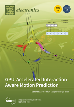
The main goal of this publication is to explore hardware acceleration techniques in the field of motion prediction for autonomous vehicles. In this paper, a set of techniques to bring a computationally expensive, state-of-the-art motion prediction algorithm to real-time execution are presented with the goal of achieving a standard motion-planning execution frequency of 5 Hz. This is achieved by applying novel and existing parallelization algorithms that take advantage of graphic processing units (GPUs) through the compute unified device architecture (CUDA) programming language and managing to produce an average 5x speedup over raw C++ in the studied cases. The optimizations are evaluated using public datasets and a real vehicle on a test track. View this paper
  • Issues are regarded as officially published after their release is announced to the table of contents alert mailing list.
  • You may sign up for e-mail alerts to receive table of contents of newly released issues.
  • PDF is the official format for papers published in both, html and pdf forms. To view the papers in pdf format, click on the "PDF Full-text" link, and use the free Adobe Reader to open them.
Order results
Result details
Section
Select all
Export citation of selected articles as:
19 pages, 582 KiB  
Article
Electrical Power Edge-End Interaction Modeling with Time Series Label Noise Learning
by Zhenshang Wang, Mi Zhou, Yuming Zhao, Fan Zhang, Jing Wang, Bin Qian, Zhen Liu, Peitian Ma and Qianli Ma
Electronics 2023, 12(18), 3987; https://doi.org/10.3390/electronics12183987 - 21 Sep 2023
Cited by 3 | Viewed by 1275
Abstract
In the context of electrical power systems, modeling the edge-end interaction involves understanding the dynamic relationship between different components and endpoints of the system. However, the time series of electrical power obtained by user terminals often suffer from low-quality issues such as missing [...] Read more.
In the context of electrical power systems, modeling the edge-end interaction involves understanding the dynamic relationship between different components and endpoints of the system. However, the time series of electrical power obtained by user terminals often suffer from low-quality issues such as missing values, numerical anomalies, and noisy labels. These issues can easily reduce the robustness of data mining results for edge-end interaction models. Therefore, this paper proposes a time–frequency noisy label classification (TF-NLC) model, which improves the robustness of edge-end interaction models in dealing with low-quality issues. Specifically, we employ two deep neural networks that are trained concurrently, utilizing both the time and frequency domains. The two networks mutually guide each other’s classification training by selecting clean labels from batches within small loss data. To further improve the robustness of the classification of time and frequency domain feature representations, we introduce a time–frequency domain consistency contrastive learning module. By classifying the selection of clean labels based on time–frequency representations for mutually guided training, TF-NLC can effectively mitigate the negative impact of noisy labels on model training. Extensive experiments on eight electrical power and ten other different realistic scenario time series datasets show that our proposed TF-NLC achieves advanced classification performance under different noisy label scenarios. Also, the ablation and visualization experiments further demonstrate the robustness of our proposed method. Full article
(This article belongs to the Special Issue Knowledge Engineering and Data Mining Volume II)
Show Figures

Figure 1

Figure 1
<p>The framework for the time–frequency noisy label classification model.</p>
Full article ">Figure 2
<p>The left plot shows the bluecurve representing a time series in C1P1 that is labeled as normal electricity consumption behavior. On the right plot, the red curve represents a series in C1P1 that is labeled as abnormal electricity consumption behavior (notably around 9 o’clock, where there is an abnormal fluctuation in the sensor readings).</p>
Full article ">Figure 3
<p>The t-SNE visualization depicts the performance of three methods on the Epilepsy dataset under 30% symmetric noise. Four classes are shown in different colors. Among these visualizations: (<b>a</b>) illustrates the data feature representation learned by one of the encoders after training, where the dual network (TT) works in the time domain; (<b>b</b>) shows the data feature representation obtained by one of the encoders after training, with the dual network (FF) working in the frequency domain; (<b>c</b>) demonstrates the data feature representation learned by the encoder (T) working in the time domain for TF-NLC; (<b>d</b>) indicates the data feature representation learned by the encoder (F) working in the frequency domain for TF-NLC. Upon comparing (<b>a</b>) with (<b>c</b>) and (<b>b</b>) with (<b>d</b>), it can be found that the feature representation learned by TF-NLC in both the time and frequency domains exhibits greater robustness as the feature representation is more compact.</p>
Full article ">Figure 4
<p>The training loss curves of the two methods on the ArrowHead dataset under the 30% symmetric noise setting are displayed. Specifically, (<b>a</b>) represents the loss curve for Vanilla, and (<b>b</b>) illustrates the loss curve for TF-NLC. The red curve corresponds to the average training loss of the noisy samples, while the blue curve represents the average training loss of the clean samples.</p>
Full article ">
23 pages, 807 KiB  
Article
Open-Source HW/SW Co-Simulation Using QEMU and GHDL for VHDL-Based SoC Design
by Giorgio Biagetti, Laura Falaschetti, Paolo Crippa, Michele Alessandrini and Claudio Turchetti
Electronics 2023, 12(18), 3986; https://doi.org/10.3390/electronics12183986 - 21 Sep 2023
Cited by 3 | Viewed by 4348
Abstract
Hardware/software co-simulation is a technique that can help design and validate digital circuits controlled by embedded processors. Co-simulation has largely been applied to system-level models, and tools for SystemC or SystemVerilog are readily available, but they are either not compatible or very cumbersome [...] Read more.
Hardware/software co-simulation is a technique that can help design and validate digital circuits controlled by embedded processors. Co-simulation has largely been applied to system-level models, and tools for SystemC or SystemVerilog are readily available, but they are either not compatible or very cumbersome to use with VHDL, the most commonly used language for FPGA design. This paper presents a direct, simple-to-use solution to co-simulate a VHDL design together with the firmware (FW) that controls it. It aims to bring the power of co-simulation to every digital designer, so it uses open-source tools, and the developed code is also open. A small patch applied to the QEMU emulator allows it to communicate with a custom-written VHDL module that exposes a CPU bus to the digital design, controlled by the FW emulated in QEMU. No changes to FW code or VHDL device code are required: with our approach, it is possible to co-simulate the very same code base that would then be implemented into an FPGA, enabling debugging, verification, and tracing capabilities that would not be possible even with the real hardware. Full article
(This article belongs to the Special Issue Embedded Systems: Fundamentals, Design and Practical Applications)
Show Figures

Figure 1

Figure 1
<p>Overview of the modules and of their interactions in a full HW/FW/SW co-simulation environment: The VHDL HW model is simulated by GHDL. The top-level design must include the DUT itself and our CPUemu entity to connect it to the AXI bus of the emulated CPU, where the RTLbridge virtual device takes care of handling the IPC protocol between QEMU and GHDL and synchronizes the two simulations. The DUT can also connect to our PTYemu entity, which emulates a serial port routed to the host by means of a PTY, for direct HW-SW interaction not mediated by QEMU. Standard QEMU-emulated peripherals can also be added to the virtual machine for other FW-SW communication channels not captured in the VHDL model. In general, no changes are required in the DUT HW model, FW code, and SW code between the co-simulation environment and a real hardware implementation.</p>
Full article ">Figure 2
<p>Example code to test the synchronization between QEMU and GHDL for an HW-driven process such as IRQ-based PWM generation. Excerpt from <tt>test-pwm.c</tt>; see the <a href="#app1-electronics-12-03986" class="html-app">Supplementary Materials</a> for the complete sources. The <tt>count_events</tt> function was meant to compute statistics of the ISR entry latency, besides counting the events, of course. The entry latency was found to be 2 clock cycles—the time required to setup an AXI read transaction—because for this short code QEMU is much faster than GHDL, and so from the VHDL point of view no time has elapsed at all between IRQ assertion and the reading of the <tt>count</tt> register.</p>
Full article ">Figure 3
<p>Waveforms resulting from co-simulating the FW shown in <a href="#electronics-12-03986-f002" class="html-fig">Figure 2</a>. <tt>value</tt> is the PWM value written by the FW, while <tt>actual</tt> is its double-buffered counterpart updated when <tt>count</tt> is reset to 0.</p>
Full article ">Figure 4
<p>UART simplified block diagram.</p>
Full article ">Figure 5
<p>UART control register bit assignment. From top (LSB) to bottom (MSB): TX and RX FIFO status and control, flow control, and individual IRQ enable flags. <span style="color:#0000FF"><span class="html-sans-serif">RW:</span></span> read/write; <span style="color:#00BFFF"><span class="html-sans-serif">RO:</span></span> read only; <span style="color:#FFA501"><span class="html-sans-serif">WO:</span></span> write only; <span style="color:#FF4500"><span class="html-sans-serif">W1C:</span></span> write 1 to clear; <span style="color:#FF4500"><span class="html-sans-serif">W1S:</span></span> write 1 to set (clears the FIFOs).</p>
Full article ">Figure 6
<p>Example code to test the interaction between C register access and VHDL bus transactions. Excerpt from <tt>test-bfm.c</tt>; see the <a href="#app1-electronics-12-03986" class="html-app">Supplementary Materials</a> for the complete sources.</p>
Full article ">Figure 7
<p>Skeleton of a VHDL test bench that instantiates our modules to allow co-simulation. Some connections are compacted for conciseness of explanation; the “•” symbol stands for a placeholder for all the 21 signals that actually constitute the AXI-Lite bus as shown in <a href="#electronics-12-03986-f004" class="html-fig">Figure 4</a> (see the <tt>cosim_tb.vhdl</tt> file in the <a href="#app1-electronics-12-03986" class="html-app">Supplementary Materials</a> for the complete source code).</p>
Full article ">Figure 8
<p>GDB session connected to the QEMU system emulator showing the looped-back serial data stored in memory by the emulated CPU after running the code listed in <a href="#electronics-12-03986-f006" class="html-fig">Figure 6</a>.</p>
Full article ">Figure 9
<p>Digital waveforms saved by GHDL during co-simulation of the loopback test. This overview spans the entire duration of the test and reports all the main signals: AXI-Lite bus lanes, UART internal control signals (see text for description), and the serial data waveform (UART TX) synthesized by the DUT being co-simulated. The full VCD file is available in the <a href="#app1-electronics-12-03986" class="html-app">Supplementary Materials</a>.</p>
Full article ">Figure 10
<p>Details of the bus transactions that occur at the beginning (top panel) and at the end (bottom panel) of the overall simulation shown in <a href="#electronics-12-03986-f009" class="html-fig">Figure 9</a>. The first part of the test was designed to test the correct implementation of all the possible bus access patterns and widths, as shown in the code excerpt. As can be seen from the “write strobe” (<tt>W strb</tt>) trace, the different C data types are correctly mapped to the corresponding access widths. Byte lanes are also correctly shifted (transactions at time 0.44 µs for the upper 16-bit and 0.58, 0.65, and 0.72 µs for non-32-bit aligned 8-bit accesses).</p>
Full article ">Figure 11
<p>Fragment of C code that interacts with a terminal emulator: initial connection detection. Excerpt from <tt>test-pty.c</tt>; see the <a href="#app1-electronics-12-03986" class="html-app">Supplementary Materials</a> for the complete sources.</p>
Full article ">Figure 12
<p>Example of an interactive terminal session (through the utility <tt>picocom</tt>) talking to the FW being emulated in QEMU by means of a PTY being simulated by GHDL. The command “help” and the characters ENQ (CTRL+E) and EOT (CTRL+D) after the “&gt;” prompt had been interactively typed on the keyboard and caused the FW to reply (and terminate simulation after processing EOT). Complete source code of the example is in the <tt>test-pty.c</tt> file.</p>
Full article ">Figure 13
<p>VHDL testbench for the DAQ system. Besides the CPUemu and PTYemu modules necessary to make the HW talk to the FW and SW, respectively, something to create the signal to be acquired by the DAQ must also be included in the testbench. The “analog model” serves this purpose and includes a low-pass filter and an “ideal” ADC to feed the DAQ with the PWM signal from TMR2, while TMR1 generates its sampling clock.</p>
Full article ">Figure 14
<p>Example FW code to test the DAQ system. See <tt>test-daq.c</tt> in the <a href="#app1-electronics-12-03986" class="html-app">Supplementary Materials</a> for register definitions, ISRs, and all the other details.</p>
Full article ">Figure 15
<p>Data saved from the SW-side of the co-simulation of the DAQ system when the FW feeds the 400 kHz PWM with a 120-point sampled sine wave, resulting in a 3.333 kHz frequency, for the first 2.4 ms; then, the PWM frequency is abruptly halved. Halving the frequency also results in halving the amplitude because the waveform lookup table remains the same. The LPF has a cut-off frequency of 5 kHz so the transition is smoothed (and there is some ringing).</p>
Full article ">Scheme 1
<p>The text-based IPC protocol used between QEMU and VHDL.</p>
Full article ">
21 pages, 4868 KiB  
Article
Optimizing Long Short-Term Memory Network for Air Pollution Prediction Using a Novel Binary Chimp Optimization Algorithm
by Sahba Baniasadi, Reza Salehi, Sepehr Soltani, Diego Martín, Parmida Pourmand and Ehsan Ghafourian
Electronics 2023, 12(18), 3985; https://doi.org/10.3390/electronics12183985 - 21 Sep 2023
Cited by 5 | Viewed by 2000
Abstract
Elevated levels of fine particulate matter (PM2.5) in the atmosphere present substantial risks to human health and welfare. The accurate assessment of PM2.5 concentrations plays a pivotal role in facilitating prompt responses by pertinent regulatory bodies to mitigate air pollution. [...] Read more.
Elevated levels of fine particulate matter (PM2.5) in the atmosphere present substantial risks to human health and welfare. The accurate assessment of PM2.5 concentrations plays a pivotal role in facilitating prompt responses by pertinent regulatory bodies to mitigate air pollution. Additionally, it furnishes indispensable information for epidemiological studies concentrating on PM2.5 exposure. In recent years, predictive models based on deep learning (DL) have offered promise in improving the accuracy and efficiency of air quality forecasts when compared to other approaches. Long short-term memory (LSTM) networks have proven to be effective in time series forecasting tasks, including air pollution prediction. However, optimizing LSTM models for enhanced accuracy and efficiency remains an ongoing research area. In this paper, we propose a novel approach that integrates the novel binary chimp optimization algorithm (BChOA) with LSTM networks to optimize air pollution prediction models. The proposed BChOA, inspired by the social behavior of chimpanzees, provides a powerful optimization technique to fine-tune the LSTM architecture and optimize its parameters. The evaluation of the results is performed using cross-validation methods such as the coefficient of determination (R2), accuracy, the root mean square error (RMSE), and receiver operating characteristic (ROC) curve. Additionally, the performance of the BChOA-LSTM model is compared against eight DL architectures. Experimental evaluations using real-world air pollution data demonstrate the superior performance of the proposed BChOA-based LSTM model compared to traditional LSTM models and other optimization algorithms. The BChOA-LSTM model achieved the highest accuracy of 96.41% on the validation datasets, making it the most successful approach. The results show that the BChOA-LSTM architecture performs better than the other architectures in terms of the  R2 convergence curve, RMSE, and accuracy. Full article
(This article belongs to the Special Issue Advances in Embedded Deep Learning Systems)
Show Figures

Figure 1

Figure 1
<p>The position vectors and their possible next locations.</p>
Full article ">Figure 2
<p>Position updating in ChOA.</p>
Full article ">Figure 3
<p>Position updating mechanism of chimps and effects of <math display="inline"><semantics> <mrow> <mo>|</mo> <mi mathvariant="bold-italic">a</mi> <mo>|</mo> </mrow> </semantics></math> on it.</p>
Full article ">Figure 4
<p>The structure of the proposed BChOA.</p>
Full article ">Figure 5
<p>The structure of the proposed BChOA-LSTM.</p>
Full article ">Figure 6
<p>The geographical location of the 22 districts of Tehran.</p>
Full article ">Figure 7
<p>The time series of the wind speed parameter.</p>
Full article ">Figure 8
<p>Refined wind speed image with Savitzky–Golay filter.</p>
Full article ">Figure 9
<p>The PM<sub>2.5</sub> pollutant level map in Tehran using the Kriging interpolation method.</p>
Full article ">Figure 10
<p>The generated map of PM<sub>2.5</sub> concentration using the proposed BChOA-LSTM model.</p>
Full article ">Figure 11
<p>A graphical depiction illustrating the comparison of algorithms by utilizing training datasets.</p>
Full article ">Figure 12
<p>A graphical depiction illustrating the comparison of algorithms by utilizing validation datasets.</p>
Full article ">Figure 13
<p>A visual comparison of the ROC curve for various architectures.</p>
Full article ">Figure 14
<p>The convergence trend of the algorithms.</p>
Full article ">
14 pages, 536 KiB  
Article
Towards Privacy-Preserving Federated Neuromorphic Learning via Spiking Neuron Models
by Bing Han, Qiang Fu and Xinliang Zhang
Electronics 2023, 12(18), 3984; https://doi.org/10.3390/electronics12183984 - 21 Sep 2023
Cited by 2 | Viewed by 1628
Abstract
Federated learning (FL) has been broadly adopted in both academia and industry in recent years. As a bridge to connect the so-called “data islands”, FL has contributed greatly to promoting data utilization. In particular, FL enables disjoint entities to cooperatively train a shared [...] Read more.
Federated learning (FL) has been broadly adopted in both academia and industry in recent years. As a bridge to connect the so-called “data islands”, FL has contributed greatly to promoting data utilization. In particular, FL enables disjoint entities to cooperatively train a shared model, while protecting each participant’s data privacy. However, current FL frameworks cannot offer privacy protection and reduce the computation overhead at the same time. Therefore, its implementation in practical scenarios, such as edge computing, is limited. In this paper, we propose a novel FL framework with spiking neuron models and differential privacy, which simultaneously provides theoretically guaranteed privacy protection and achieves low energy consumption. We model the local forward propagation process in a discrete way similar to nerve signal travel in the human brain. Since neurons only fire when the accumulated membrane potential exceeds a threshold, spiking neuron models require significantly lower energy compared to traditional neural networks. In addition, to protect sensitive information in model gradients, we add differently private noise in both the local training phase and server aggregation phase. Empirical evaluation results show that our proposal can effectively reduce the accuracy of membership inference attacks and property inference attacks, while maintaining a relatively low energy cost. blueFor example, the attack accuracy of a membership inference attack drops to 43% in some scenarios. As a result, our proposed FL framework can work well in large-scale cross-device learning scenarios. Full article
(This article belongs to the Special Issue Data Privacy and Cybersecurity in Mobile Crowdsensing)
Show Figures

Figure 1

Figure 1
<p>Our proposed training framework at a high level.</p>
Full article ">Figure 2
<p>Change in global model accuracy with the increase in communication rounds (CIFAR-10, M2).</p>
Full article ">
12 pages, 16406 KiB  
Article
A Study on Webtoon Generation Using CLIP and Diffusion Models
by Kyungho Yu, Hyoungju Kim, Jeongin Kim, Chanjun Chun and Pankoo Kim
Electronics 2023, 12(18), 3983; https://doi.org/10.3390/electronics12183983 - 21 Sep 2023
Viewed by 2769
Abstract
This study focuses on harnessing deep-learning-based text-to-image transformation techniques to help webtoon creators’ creative outputs. We converted publicly available datasets (e.g., MSCOCO) into a multimodal webtoon dataset using CartoonGAN. First, the dataset was leveraged for training contrastive language image pre-training (CLIP), a model [...] Read more.
This study focuses on harnessing deep-learning-based text-to-image transformation techniques to help webtoon creators’ creative outputs. We converted publicly available datasets (e.g., MSCOCO) into a multimodal webtoon dataset using CartoonGAN. First, the dataset was leveraged for training contrastive language image pre-training (CLIP), a model composed of multi-lingual BERT and a Vision Transformer that learnt to associate text with images. Second, a pre-trained diffusion model was employed to generate webtoons through text and text-similar image input. The webtoon dataset comprised treatments (i.e., textual descriptions) paired with their corresponding webtoon illustrations. CLIP (operating through contrastive learning) extracted features from different data modalities and aligned similar data more closely within the same feature space while pushing dissimilar data apart. This model learnt the relationships between various modalities in multimodal data. To generate webtoons using the diffusion model, the process involved providing the CLIP features of the desired webtoon’s text with those of the most text-similar image to a pre-trained diffusion model. Experiments were conducted using both single- and continuous-text inputs to generate webtoons. In the experiments, both single-text and continuous-text inputs were used to generate webtoons, and the results showed an inception score of 7.14 when using continuous-text inputs. The text-to-image technology developed here could streamline the webtoon creation process for artists by enabling the efficient generation of webtoons based on the provided text. However, the current inability to generate webtoons from multiple sentences or images while maintaining a consistent artistic style was noted. Therefore, further research is imperative to develop a text-to-image model capable of handling multi-sentence and -lingual input while ensuring coherence in the artistic style across the generated webtoon images. Full article
(This article belongs to the Special Issue Machine Learning and Deep Learning Based Pattern Recognition)
Show Figures

Figure 1

Figure 1
<p>The training process of the diffusion model.</p>
Full article ">Figure 2
<p>The structure of CLIP and an example of the logits matrix for a text–image pair.</p>
Full article ">Figure 3
<p>Calculation method of consine similarity in the pseudocode of CLIP.</p>
Full article ">Figure 4
<p>Method for calculating accuracy in the pseudocode of CLIP.</p>
Full article ">Figure 5
<p>Graph of accuracy (<b>a</b>) and loss (<b>b</b>) during CLIP training on the train dataset. Graph of accuracy (<b>c</b>) and loss (<b>d</b>) during CLIP training on the validation dataset. The x-axis of accuracy (<b>a</b>,<b>c</b>) represents the training steps, and the y-axis represents accuracy. For loss (<b>b</b>,<b>d</b>) the x-axis represents training steps, and the y-axis represents loss.</p>
Full article ">
16 pages, 3630 KiB  
Technical Note
A Novel DME-YOLO Structure in a High-Frequency Transformer Improves the Accuracy and Speed of Detection
by Zhiqiang Kang, Wenqian Jiang, Lile He and Chenrui Zhang
Electronics 2023, 12(18), 3982; https://doi.org/10.3390/electronics12183982 - 21 Sep 2023
Cited by 1 | Viewed by 1801
Abstract
Traditional YOLO models face a dilemma when it comes to dim detection targets: the detection accuracy increases while the speed inevitably reduces, or vice versa. To resolve this issue, we propose a novel DME-YOLO model, which is characterized by the establishment of a [...] Read more.
Traditional YOLO models face a dilemma when it comes to dim detection targets: the detection accuracy increases while the speed inevitably reduces, or vice versa. To resolve this issue, we propose a novel DME-YOLO model, which is characterized by the establishment of a backbone based on the YOLOv7 and Dense blocks. Moreover, through the application of feature multiplexing, both the parameters and floating-point computation were decreased; therefore, the defect detection process was accelerated. We also designed a multi-source attention mechanism module called MSAM, which is capable of integrating spatial information from multiple sources. Due to its outstanding quality, the addition of MSAM as the neck of the original YOLOv7 model compensated for the loss of spatial information in the process of forward propagation, thereby improving the detection accuracy of small target defects and simultaneously ensuring real-time detection. Finally, EIOU was adopted as a loss function to bolster the target frame regression process. The results of the experiment indicated detection accuracy and speed values of up to 97.6 mAP and 51.2 FPS, respectively, suggesting the superiority of the model. Compared with the YOLOv7 model, the experimental parameters for the novel DME-YOLO increased by 2.8% for mAP and 15.7 for FPS, respectively. In conclusion, the novel DME-YOLO model had excellent overall performance regarding detection speed and accuracy. Full article
(This article belongs to the Special Issue Advances and Applications of Computer Vision in Electronics)
Show Figures

Figure 1

Figure 1
<p>Some high-frequency transformers with surface defects.</p>
Full article ">Figure 2
<p>The original architecture of YOLOv7.</p>
Full article ">Figure 3
<p>Comparison between the ELAN block and Dense block.</p>
Full article ">Figure 4
<p>Multi-Source Space Attention Module.</p>
Full article ">Figure 5
<p>The MSAM-YOLO architecture.</p>
Full article ">Figure 6
<p>The overall architecture of MSAM.</p>
Full article ">Figure 7
<p>Mosaic data augmentation.</p>
Full article ">Figure 8
<p>Results of detection.</p>
Full article ">Figure 9
<p>Grad-CAM thermal region.</p>
Full article ">Figure 10
<p>Four locations on the neck for attention.</p>
Full article ">
17 pages, 4959 KiB  
Article
Target Localization and Grasping of NAO Robot Based on YOLOv8 Network and Monocular Ranging
by Yingrui Jin, Zhaoyuan Shi, Xinlong Xu, Guang Wu, Hengyi Li and Shengjun Wen
Electronics 2023, 12(18), 3981; https://doi.org/10.3390/electronics12183981 - 21 Sep 2023
Cited by 10 | Viewed by 2522
Abstract
As a typical visual positioning system, monocular ranging is widely used in various fields. However, when the distance increases, there is a greater error. YOLOv8 network has the advantages of fast recognition speed and high accuracy. This paper proposes a method by combining [...] Read more.
As a typical visual positioning system, monocular ranging is widely used in various fields. However, when the distance increases, there is a greater error. YOLOv8 network has the advantages of fast recognition speed and high accuracy. This paper proposes a method by combining YOLOv8 network recognition with a monocular ranging method to achieve target localization and grasping for the NAO robots. By establishing a visual distance error compensation model and applying it to correct the estimation results of the monocular distance measurement model, the accuracy of the NAO robot’s long-distance monocular visual positioning is improved. Additionally, a grasping control strategy based on pose interpolation is proposed. Throughout, the proposed method’s advantage in measurement accuracy was confirmed via experiments, and the grasping strategy has been implemented to accurately grasp the target object. Full article
Show Figures

Figure 1

Figure 1
<p>Schematic diagram of monocular ranging based on YOLOv8.</p>
Full article ">Figure 2
<p>The structure of YOLOv8 network.</p>
Full article ">Figure 3
<p>The pinhole imaging model.</p>
Full article ">Figure 4
<p>The monocular ranging model for the NAO robot.</p>
Full article ">Figure 5
<p>Vertical view of the monocular ranging model.</p>
Full article ">Figure 6
<p>Relationship between the <math display="inline"><semantics> <mrow> <mi>γ</mi> </mrow> </semantics></math> angle and the measured distance.</p>
Full article ">Figure 7
<p>Relationship between the measured distance and error coefficient <math display="inline"><semantics> <mrow> <mi>k</mi> </mrow> </semantics></math>.</p>
Full article ">Figure 8
<p>Gaussian process regression result.</p>
Full article ">Figure 9
<p>Interpolation curves for displacement, velocity, and acceleration.</p>
Full article ">Figure 10
<p>Linear motion interpolation diagram.</p>
Full article ">Figure 11
<p>Joint angle motion curves.</p>
Full article ">Figure 12
<p>D-H model of NAO robot’s right arm.</p>
Full article ">Figure 13
<p>(<b>a</b>) Original image captured by NAO robot; (<b>b</b>) Target object identified by YOLOv8.</p>
Full article ">Figure 14
<p>(<b>a</b>) Endpoints of the target object; (<b>b</b>) Edge of the target object.</p>
Full article ">Figure 15
<p>Comparison of measured distances before and after error compensation.</p>
Full article ">Figure 16
<p>NAO robot grasping process.</p>
Full article ">
19 pages, 3408 KiB  
Article
Convolutional Neural Networks Adapted for Regression Tasks: Predicting the Orientation of Straight Arrows on Marked Road Pavement Using Deep Learning and Rectified Orthophotography
by Calimanut-Ionut Cira, Alberto Díaz-Álvarez, Francisco Serradilla and Miguel-Ángel Manso-Callejo
Electronics 2023, 12(18), 3980; https://doi.org/10.3390/electronics12183980 - 21 Sep 2023
Cited by 5 | Viewed by 3896
Abstract
Arrow signs found on roadway pavement are an important component of modern transportation systems. Given the rise in autonomous vehicles, public agencies are increasingly interested in accurately identifying and analysing detailed road pavement information to generate comprehensive road maps and decision support systems [...] Read more.
Arrow signs found on roadway pavement are an important component of modern transportation systems. Given the rise in autonomous vehicles, public agencies are increasingly interested in accurately identifying and analysing detailed road pavement information to generate comprehensive road maps and decision support systems that can optimise traffic flow, enhance road safety, and provide complete official road cartographic support (that can be used in autonomous driving tasks). As arrow signs are a fundamental component of traffic guidance, this paper aims to present a novel deep learning-based approach to identify the orientation and direction of arrow signs on marked roadway pavements using high-resolution aerial orthoimages. The approach is based on convolutional neural network architectures (VGGNet, ResNet, Xception, and DenseNet) that are modified and adapted for regression tasks with a proposed learning structure, together with an ad hoc model, specially introduced for this task. Although the best-performing artificial neural network was based on VGGNet (VGG-19 variant), it only slightly surpassed the proposed ad hoc model in the average values of the R2 score, mean squared error, and angular error by 0.005, 0.001, and 0.036, respectively, using the training set (the ad hoc model delivered an average R2 score, mean squared error, and angular error of 0.9874, 0.001, and 2.516, respectively). Furthermore, the ad hoc model’s predictions using the test set were the most consistent (a standard deviation of the R2 score of 0.033 compared with the score of 0.042 achieved using VGG19), while being almost eight times more computationally efficient when compared with the VGG19 model (2,673,729 parameters vs VGG19′s 20,321,985 parameters). Full article
(This article belongs to the Special Issue Advances in Computer Vision and Deep Learning and Its Applications)
Show Figures

Figure 1

Figure 1
<p>Process diagram showing the workflow applied in this study that includes the generation of an arrow dataset from orthophotography and the evaluation method to determine the final selected model.</p>
Full article ">Figure 2
<p>Proposed procedure for generating the dataset containing arrow signs found on pavement and their corresponding orientation label.</p>
Full article ">Figure 3
<p>The proposed ad hoc architecture is based on CNN learning structures together with the proposed CNN adaptation for regression tasks.</p>
Full article ">Figure 4
<p>Example showing the distribution of bootstrapped R<sup>2</sup> values for one of the neural networks trained in this study (the modified VGG19 model).</p>
Full article ">Figure 5
<p>Examples of tiles belonging to the RoadArrowORIEN dataset (used for training and testing the artificial neural networks), together with their corresponding angular value.</p>
Full article ">Figure 6
<p>Illustration showing the VGG-16 and VGG-19 architectures. Note: VGG-16 is equivalent to VGG-19 but without the “CONV_3-4”, “CONV_4-4”, and “CONV_5-4” layers. Note: for training, the classifier part (the last three FC layers) was replaced with the inference block of the orientation angle proposed in <a href="#sec3dot2-electronics-12-03980" class="html-sec">Section 3.2</a>.</p>
Full article ">Figure 7
<p>The ResNet-50 architecture consists of 50 layers, including convolutional layers, pooling layers, residual blocks, and a global average pooling layer. Note: for training, the last FC layer was replaced with the inference block of the orientation angle proposed in <a href="#sec3dot2-electronics-12-03980" class="html-sec">Section 3.2</a>.</p>
Full article ">Figure 8
<p>The Xception architecture consists of a series of convolutional and depth-wise separable convolutional layers, with skip connections, batch normalisation, and global average pooling. Note: for training, the last FC layer was replaced with the inference block of the orientation angle proposed in <a href="#sec3dot2-electronics-12-03980" class="html-sec">Section 3.2</a>.</p>
Full article ">Figure 9
<p>A schematic representation showing the DenseNet architecture, illustrating the information flow through the densely connected layers (based on [<a href="#B4-electronics-12-03980" class="html-bibr">4</a>]). Between the three dense blocks, two adjacent blocks are referred to as transition layers, which change feature-map sizes via convolutional and pooling layers. Note: For training, the classifier part was replaced with the inference block of the orientation angle proposed in <a href="#sec3dot2-electronics-12-03980" class="html-sec">Section 3.2</a>.</p>
Full article ">Figure 10
<p>Visual representation showing the performance metrics achieved on the test set using the trained models in terms of (<b>a</b>) R<sup>2</sup> score, (<b>b</b>) MSE, and (<b>c</b>) angular error. Note: The intervals represent the values obtained from applying the bootstrapping training procedure (described in <a href="#sec3dot3-electronics-12-03980" class="html-sec">Section 3.3</a>).</p>
Full article ">Figure 11
<p>(<b>a</b>–<b>f</b>) Random samples featuring high predicted angular error (superior to 30 degrees) that were obtained using the ad hoc model.</p>
Full article ">
21 pages, 6773 KiB  
Article
Comparison of 2L + 2M and 6L SVPWM for Five-Phase Inverter to Reduce Common Mode Voltage
by Kotb B. Tawfiq, Arafa S. Mansour and Peter Sergeant
Electronics 2023, 12(18), 3979; https://doi.org/10.3390/electronics12183979 - 21 Sep 2023
Cited by 2 | Viewed by 1516
Abstract
Multiphase drives have received a lot of interest because of their several features over traditional three-phase systems for high-power applications. Pulse-width modulation (PWM) approaches are necessary to regulate the supply for multiphase ac drives. As a result, it is vital to continually improve [...] Read more.
Multiphase drives have received a lot of interest because of their several features over traditional three-phase systems for high-power applications. Pulse-width modulation (PWM) approaches are necessary to regulate the supply for multiphase ac drives. As a result, it is vital to continually improve the modulation and control approaches used to upgrade output power converters’ quality. This paper offers a comparative analysis of the 2L + 2M and 6L space vector pulse-width modulation (SVPWM) techniques applied to a five-phase two-level voltage source inverter (VSI) fed an inductive (R-L) load. The comparative evaluation is based on measuring the inverter switching losses, the total harmonic distortion (THD) values, and the common mode voltage (CMV) under different operation scenarios. A system model is carried out by MATLAB/Simulink. An experimental prototype is constructed in the lab to validate the theoretical analysis. Simulation results for the system based on the two SVPWM techniques are obtained at different modulation indices and different output frequencies and are confirmed by the experimental results. It has been found that the peak-to-peak CMV of the 6L method is 80% lower than that of the 2L + 2M method. Moreover, 6L SVPWM offers better DC-link utilization compared to 2L + 2M SVPWM. Full article
(This article belongs to the Special Issue Power Electronic Converters in a Multiphase Drive Systems)
Show Figures

Figure 1

Figure 1
<p>Two-level five-phase VSI.</p>
Full article ">Figure 2
<p>Switching voltage space vectors in the <span class="html-italic">α–β</span> plane.</p>
Full article ">Figure 3
<p>The 2L + 2M switching pattern for the top switches of the five-phase VSI in the first sector.</p>
Full article ">Figure 4
<p>The 6L switching pattern in the α–β plane.</p>
Full article ">Figure 5
<p>The 6L switching arrangement for the top switches of the five-phase VSI in the first zone.</p>
Full article ">Figure 6
<p>Simulation results of the CMV at unity modulation index and 50 Hz for (<b>a</b>) 2L + 2M and (<b>b</b>) 6L methods.</p>
Full article ">Figure 7
<p>Simulation results of the output phase voltages at unity modulation index and 50 Hz for (<b>a</b>) 2L + 2M and (<b>b</b>) 6L methods.</p>
Full article ">Figure 7 Cont.
<p>Simulation results of the output phase voltages at unity modulation index and 50 Hz for (<b>a</b>) 2L + 2M and (<b>b</b>) 6L methods.</p>
Full article ">Figure 8
<p>Simulation results of the output line-to-line voltages at unity modulation index and 50 Hz for (<b>a</b>) 2L + 2M and (<b>b</b>) 6L methods.</p>
Full article ">Figure 8 Cont.
<p>Simulation results of the output line-to-line voltages at unity modulation index and 50 Hz for (<b>a</b>) 2L + 2M and (<b>b</b>) 6L methods.</p>
Full article ">Figure 9
<p>Simulation results of the output phase currents at unity modulation index and 50 Hz for (<b>a</b>) 2L + 2M and (<b>b</b>) 6L methods.</p>
Full article ">Figure 10
<p>Simulation results of the THD of the output phase currents for 2L + 2M and 6L methods at 50 Hz and modulation indices of (<b>a</b>) 1 and (<b>b</b>) 0.5.</p>
Full article ">Figure 11
<p>Simulation results of the inverter switching and conduction losses at unity modulation index and 50 Hz.</p>
Full article ">Figure 12
<p>Simulation results of the output phase currents at unity modulation index and 25 Hz for (<b>a</b>) 2L + 2M and (<b>b</b>) 6L methods.</p>
Full article ">Figure 13
<p>Simulation results of the output line-to-line voltage at unity modulation index and 25 Hz for (<b>a</b>) 2L + 2M and (<b>b</b>) 6L methods.</p>
Full article ">Figure 14
<p>Photo of the experimental setup.</p>
Full article ">Figure 15
<p>Experimental and simulation results of the CMV at unity modulation index and 50 Hz for (<b>a</b>) simulation of 2L + 2M method, (<b>b</b>) experiment of 2L + 2M method, (<b>c</b>) simulation of 6L method, and (<b>d</b>) experiment of 6L method.</p>
Full article ">Figure 16
<p>Experimental and simulation results of the output phase voltages at unity modulation index and 50 Hz for 2L + 2M (<b>a</b>) simulation and (<b>b</b>) experiment.</p>
Full article ">Figure 16 Cont.
<p>Experimental and simulation results of the output phase voltages at unity modulation index and 50 Hz for 2L + 2M (<b>a</b>) simulation and (<b>b</b>) experiment.</p>
Full article ">Figure 17
<p>Experimental and simulation results of the output phase voltages at unity modulation index and 50 Hz for 6L (<b>a</b>) simulation and (<b>b</b>) experiment.</p>
Full article ">Figure 17 Cont.
<p>Experimental and simulation results of the output phase voltages at unity modulation index and 50 Hz for 6L (<b>a</b>) simulation and (<b>b</b>) experiment.</p>
Full article ">Figure 18
<p>Experimental and simulation results of the output line-to-line voltages at unity modulation index and 50 Hz for 2L + 2M method’s (<b>a</b>) simulation results and (<b>b</b>) experimental results.</p>
Full article ">Figure 18 Cont.
<p>Experimental and simulation results of the output line-to-line voltages at unity modulation index and 50 Hz for 2L + 2M method’s (<b>a</b>) simulation results and (<b>b</b>) experimental results.</p>
Full article ">Figure 19
<p>Experimental and simulation results of the output line-to-line voltages at unity modulation index and 50 Hz for 6L method’s (<b>a</b>) simulation results and (<b>b</b>) experimental results.</p>
Full article ">Figure 19 Cont.
<p>Experimental and simulation results of the output line-to-line voltages at unity modulation index and 50 Hz for 6L method’s (<b>a</b>) simulation results and (<b>b</b>) experimental results.</p>
Full article ">Figure 20
<p>Experimental and simulation results of the output phase currents at unity modulation index and 50 Hz: (<b>a</b>) simulation results of 2L + 2M method, (<b>b</b>) experimental results of 2L + 2M method, (<b>c</b>) simulation results of 6L method, and (<b>d</b>) experimental results of 6L method.</p>
Full article ">Figure 21
<p>Experimental results of the output phase currents at unity modulation index and 25 Hz: (<b>a</b>) simulation results of 2L + 2M method, (<b>b</b>) experimental results of 2L + 2M method, (<b>c</b>) simulation results of 6L method, and (<b>d</b>) experimental results of 6L method.</p>
Full article ">
19 pages, 9083 KiB  
Article
A Deep Learning-Enhanced Stereo Matching Method and Its Application to Bin Picking Problems Involving Tiny Cubic Workpieces
by Masaru Yoshizawa, Kazuhiro Motegi and Yoichi Shiraishi
Electronics 2023, 12(18), 3978; https://doi.org/10.3390/electronics12183978 - 21 Sep 2023
Viewed by 1457
Abstract
This paper proposes a stereo matching method enhanced by object detection and instance segmentation results obtained through the use of a deep convolutional neural network. Then, this method is applied to generate a picking plan to solve bin picking problems, that is, to [...] Read more.
This paper proposes a stereo matching method enhanced by object detection and instance segmentation results obtained through the use of a deep convolutional neural network. Then, this method is applied to generate a picking plan to solve bin picking problems, that is, to automatically pick up objects with random poses in a stack using a robotic arm. The system configuration and bin picking process flow are suggested using the proposed method, and it is applied to bin picking problems, especially those involving tiny cubic workpieces. The picking plan is generated by applying the Harris corner detection algorithm to the point cloud in the generated three-dimensional map. In the experiments, two kinds of stacks consisting of cubic workpieces with an edge length of 10 mm or 5 mm are tested for bin picking. In the first bin picking problem, all workpieces are successfully picked up, whereas in the second, the depths of the workpieces are obtained, but the instance segmentation process is not completed. In future work, not only cubic workpieces but also other arbitrarily shaped workpieces should be recognized in various types of bin picking problems. Full article
(This article belongs to the Special Issue Recent Advances in Object Detection and Image Processing)
Show Figures

Figure 1

Figure 1
<p>Example of a workpiece being mounted on a 3-D board using a robotic arm.</p>
Full article ">Figure 2
<p>Future assembly work with tiny workpieces.</p>
Full article ">Figure 3
<p>Images obtained using a depth camera.</p>
Full article ">Figure 4
<p>Image obtained using a 3D scanner.</p>
Full article ">Figure 5
<p>Bin picking problem and tiny workpieces.</p>
Full article ">Figure 6
<p>Suggested system configuration.</p>
Full article ">Figure 7
<p>Process flow of the proposed system.</p>
Full article ">Figure 8
<p>Synthesis of depth values and instance segmentation.</p>
Full article ">Figure 9
<p>Rotational angle calculation.</p>
Full article ">Figure 10
<p>Contact estimation of the end effector with workpieces.</p>
Full article ">Figure 11
<p>Experimental system.</p>
Full article ">Figure 12
<p>Bin picking problem for the experiment.</p>
Full article ">Figure 13
<p>Image of a stack of workpieces used for training.</p>
Full article ">Figure 14
<p>Object detection and instance segmentation results for the bin picking problem.</p>
Full article ">Figure 15
<p>Obtained result using conventional stereo matching.</p>
Full article ">Figure 16
<p>Detected corner point candidates using the “cornerHarris” function.</p>
Full article ">Figure 17
<p>First picking selection.</p>
Full article ">Figure 18
<p>Second picking process.</p>
Full article ">Figure 19
<p>Bin picking process for the final stage.</p>
Full article ">Figure 20
<p>Example of picking by the robotic arm, and the first workpiece is picked up as shown in the processes from (<b>a</b>) to (<b>f</b>).</p>
Full article ">Figure 21
<p>Example of a bin picking problem consisting of tinier workpieces.</p>
Full article ">Figure 22
<p>Input images and instance segmentation results in each stage.</p>
Full article ">Figure 23
<p>Workpieces with recognition failure.</p>
Full article ">Figure 24
<p>Picking process by the robotic arm in the first stage, and the target workpiece is picked up as shown in the processes from (<b>a</b>) to (<b>c</b>).</p>
Full article ">
14 pages, 1476 KiB  
Article
Property Analysis of Gateway Refinement of Object-Oriented Petri Net with Inhibitor-Arcs-Based Representation for Embedded Systems
by Chuanliang Xia, Mengying Qin, Yan Sun and Maibo Guo
Electronics 2023, 12(18), 3977; https://doi.org/10.3390/electronics12183977 - 21 Sep 2023
Viewed by 1147
Abstract
This paper focuses on embedded system modeling, proposing a solution to obtain a refined net via the refinement operation of an extended Petri net. Object-oriented technology and Petri net with inhibitor-arcs-based representation for embedded systems (PIRES+) are combined to obtain an object-oriented PIRES+ [...] Read more.
This paper focuses on embedded system modeling, proposing a solution to obtain a refined net via the refinement operation of an extended Petri net. Object-oriented technology and Petri net with inhibitor-arcs-based representation for embedded systems (PIRES+) are combined to obtain an object-oriented PIRES+ (OOPIRES+). A gateway refinement method of OOPIRES+ is proposed, and the preservation of the liveness, boundedness, reachability, functionality, and timing of the refined net system is investigated. The modeling analysis of a smart home system is taken as an example to verify the effectiveness of the refinement method. The results can provide an effective way for the investigation of the refined properties of a Petri net system and a favorable means for large-scale complex embedded system modeling, which has broad application prospects. Full article
(This article belongs to the Special Issue Deep Learning for Data Mining: Theory, Methods, and Applications)
Show Figures

Figure 1

Figure 1
<p>An example of the PIRES+ model.</p>
Full article ">Figure 2
<p>An example of the OOPIRES+ object subnet.</p>
Full article ">Figure 3
<p>Gateway refinement operation schematic diagram of the OOPIRES+ net system.</p>
Full article ">Figure 4
<p>Abstract model <math display="inline"><semantics> <mrow> <mi>OPN</mi> </mrow> </semantics></math> of the system.</p>
Full article ">Figure 5
<p>The object subnet <math display="inline"><semantics> <mrow> <msub> <mrow> <mi>OPSN</mi> </mrow> <mi mathvariant="normal">A</mi> </msub> </mrow> </semantics></math>.</p>
Full article ">Figure 6
<p>The object subnet <math display="inline"><semantics> <mrow> <msub> <mrow> <mi>OPSN</mi> </mrow> <mrow> <mi>AA</mi> </mrow> </msub> </mrow> </semantics></math>.</p>
Full article ">Figure 7
<p>The refined smart home remote control system <math display="inline"><semantics> <mrow> <msub> <mrow> <mi>OPN</mi> </mrow> <mi mathvariant="normal">B</mi> </msub> </mrow> </semantics></math>.</p>
Full article ">Figure 8
<p>Verification result of liveness and boundedness of <math display="inline"><semantics> <mrow> <mi>OPN</mi> </mrow> </semantics></math>.</p>
Full article ">Figure 9
<p>Verification result of liveness and boundedness of <math display="inline"><semantics> <mrow> <msub> <mrow> <mi>OPN</mi> </mrow> <mi mathvariant="normal">B</mi> </msub> </mrow> </semantics></math>.</p>
Full article ">
17 pages, 5460 KiB  
Article
An Objective Holographic Feedback Linearization Based on a Sliding Mode Control for a Buck Converter with a Constant Power Load
by Jiyong Li, Benquan Pi, Pengcheng Zhou, Jingwen Li, Hao Dong and Peiwen Chen
Electronics 2023, 12(18), 3976; https://doi.org/10.3390/electronics12183976 - 21 Sep 2023
Viewed by 1185
Abstract
As a typical load, the constant power load (CPL) has negative impedance characteristics. The stability of the buck converter system with a mixed load of CPL and resistive load is affected by the size of the CPL. When the resistive load is larger [...] Read more.
As a typical load, the constant power load (CPL) has negative impedance characteristics. The stability of the buck converter system with a mixed load of CPL and resistive load is affected by the size of the CPL. When the resistive load is larger than the CPL, the buck converter with the output voltage as an output function is a non-minimum phase nonlinear system, because its linear approximation has a right-half-plane pole. The non-minimum phase characteristic limits the application of many control techniques, but the objective holographic feedback linearization control (OHFLC) method is a good control strategy that can bypass the non-minimum phase system and make the system stable. However, the traditional OHFLC method, in designing the controller, generally uses a linear optimal quadratic design method to obtain a linear feedback control law. It requires a state quantity component with a one-order relative degree to the system. But it is not easy to find such a suitable state quantity with a one-order relative degree to the system. In this paper, an improved OHFLC method is proposed for Buck converters with a mixed loads of CPL and resistive loads, using the sliding mode control (SMC) theory to design the controller, so that the output state quantity components with different relative degrees to the system can be used in the holographic feedback linearization method. Finally, the simulation and experimental results also demonstrate that this method has the same, or even better, dynamic response performance and robustness than the traditional OHFLC method. Full article
(This article belongs to the Special Issue Advanced Control Techniques of Power Electronics)
Show Figures

Figure 1

Figure 1
<p>Main circuit diagram of Buck converter.</p>
Full article ">Figure 2
<p>Graphical representation of the sliding mode process.</p>
Full article ">Figure 3
<p>Closed-loop control block diagram of Buck converter with OHFL based on SMC.</p>
Full article ">Figure 4
<p>Simulation waveforms when CPL changes in the two situations and traditional OHFLC: (<b>a</b>) voltage waveforms, (<b>b</b>) current waveforms.</p>
Full article ">Figure 5
<p>Simulation waveforms when <span class="html-italic">R</span> changes in the two situations and traditional OHFLC: (<b>a</b>) voltage waveforms, (<b>b</b>) current waveforms.</p>
Full article ">Figure 6
<p>Experimental platform.</p>
Full article ">Figure 7
<p>System dynamic responses when the CPL increases: (<b>a</b>) waveform in situation ①, (<b>b</b>) waveform in situation ②.</p>
Full article ">Figure 8
<p>System dynamic responses when the CPL decreases: (<b>a</b>) waveform in situation ①, (<b>b</b>) waveform in situation ②.</p>
Full article ">Figure 9
<p>System dynamic responses when the <span class="html-italic">R</span> decreases: (<b>a</b>) waveform in situation ①, (<b>b</b>) waveform in situation ②.</p>
Full article ">Figure 10
<p>System dynamic responses when the <span class="html-italic">R</span> increases: (<b>a</b>) waveform in situation ①, (<b>b</b>) waveform in situation ②.</p>
Full article ">
20 pages, 11052 KiB  
Article
A High-Power Density DC Converter for Medium-Voltage DC Distribution Networks
by Dai Wan, Qianfan Zhou, Xujin Duan, Jiran Zhu, Junhao Li and Hengyi Zhou
Electronics 2023, 12(18), 3975; https://doi.org/10.3390/electronics12183975 - 21 Sep 2023
Cited by 3 | Viewed by 1719
Abstract
A DC converter is the core equipment of voltage conversion and power distribution in a DC distribution network. Its operating characteristics have a profound impact on the flexible regulation of distributed resources in an active distribution network. It is challenging for the existing [...] Read more.
A DC converter is the core equipment of voltage conversion and power distribution in a DC distribution network. Its operating characteristics have a profound impact on the flexible regulation of distributed resources in an active distribution network. It is challenging for the existing single-stage conversion topology to meet the requirements of distributed renewable energy connected to a multi-voltage level, medium-voltage grid. It is necessary to study the multistage transform power unit topology further, which can satisfy high reliability, high efficiency, and wide input range. This paper proposes a high-power density DC converter for medium-voltage DC networks with wide voltage levels. It adopts Buck-LLC integrated modular composition. The input ends of the high isolation resonant power unit are connected in series to provide high voltage endurance, and the output ends are connected in parallel to meet the high-power demand and achieve high-power transmission efficiency. The proposed series dual Buck-LLC resonant power unit topology can adjust the duty cycle of series dual buck circuits to meet the needs of different levels of medium-voltage DC power grids. The soft switching problem within the wide input range of all switching tubes is solved by introducing auxiliary inductors, thereby improving energy transmission efficiency. The auxiliary circuit and control parameters are optimized based on the research of each switching tube’s soft switching boundary conditions. Finally, an experimental prototype of a 6.25~7 kW power unit is designed and developed to prove the proposed topology’s feasibility and effectiveness. Great breakthroughs have been made both in theoretical research and engineering prototype development. Full article
Show Figures

Figure 1

Figure 1
<p>Modular combined DC-DC converter based on Buck-LLC integration.</p>
Full article ">Figure 2
<p>Waveforms of each operational mode of SDBuck-LLC.</p>
Full article ">Figure 3
<p>Key voltage and current waveforms of SDBuck-LLC (<b>a</b>) mode X1 and (<b>b</b>) mode Y2.</p>
Full article ">Figure 4
<p>Equivalent circuits of stage 1 and stage 2 in mode X1.</p>
Full article ">Figure 5
<p>Equivalent circuits of stage 3 and stage 4 in mode X1.</p>
Full article ">Figure 6
<p>Equivalent circuits of stage 5 and stage 6 in mode X1.</p>
Full article ">Figure 7
<p>Equivalent circuits of stage 7, stage 8, and stage 9 in mode X1.</p>
Full article ">Figure 7 Cont.
<p>Equivalent circuits of stage 7, stage 8, and stage 9 in mode X1.</p>
Full article ">Figure 8
<p>Steady-state equivalent circuit of SDBuck-LLC.</p>
Full article ">Figure 9
<p>The relationship between power <span class="html-italic">P</span> and <span class="html-italic">D</span><sub>1</sub>, <span class="html-italic">L</span><sub>b</sub> under different phase shifts <span class="html-italic">φT</span><sub>s</sub>.</p>
Full article ">Figure 10
<p>The relationship between <span class="html-italic">I</span><sub>S5on</sub> and <span class="html-italic">D</span><sub>1</sub>, <span class="html-italic">L</span><sub>b</sub> under different phase shifts <span class="html-italic">φT</span><sub>s</sub>.</p>
Full article ">Figure 11
<p>The relationship between <span class="html-italic">I</span><sub>S6on</sub> and <span class="html-italic">D</span><sub>1</sub>, <span class="html-italic">L</span><sub>b</sub> under different phase shifts <span class="html-italic">φT</span><sub>s</sub>.</p>
Full article ">Figure 12
<p>The relationship between <span class="html-italic">I</span><sub>S1on</sub>, <span class="html-italic">I</span><sub>S4on</sub>, and <span class="html-italic">D</span><sub>1</sub>, <span class="html-italic">L</span><sub>b</sub> under different phase shifts <span class="html-italic">φT</span><sub>s</sub>.</p>
Full article ">Figure 13
<p>Experimental prototype of SDBuck-LLC.</p>
Full article ">Figure 14
<p>Steady-state experimental waveform of SDBuck-LLC with an output power of 6.25 kW under different <span class="html-italic">V</span><sub>i</sub>.</p>
Full article ">Figure 15
<p>Steady-state experimental waveforms of SDBuck-LLC with an output power of 6.25 kW and input voltage of 1400 V.</p>
Full article ">Figure 16
<p>ZVS waveforms of each switch under full load and different input voltages <span class="html-italic">V</span><sub>i</sub>.</p>
Full article ">Figure 17
<p>ZVS waveforms of each switch under light load and different input voltages <span class="html-italic">V</span><sub>i</sub>.</p>
Full article ">Figure 18
<p>Efficiency curves of SDBuck-LLC under different input voltages <span class="html-italic">V</span><sub>i</sub>.</p>
Full article ">
15 pages, 1483 KiB  
Article
Miniaturized Dual-Band SIW-Based Bandpass Filters Using Open-Loop Ring Resonators
by Nrusingha Charan Pradhan, Slawomir Koziel, Rusan Kumar Barik, Anna Pietrenko-Dabrowska and Sholampettai Subramanian Karthikeyan
Electronics 2023, 12(18), 3974; https://doi.org/10.3390/electronics12183974 - 21 Sep 2023
Cited by 12 | Viewed by 2400
Abstract
This article presents two novel architectures of dual-band substrate-integrated waveguide (SIW) bandpass filters (BPFs). Initially, two identical open-loop ring resonators (OLRRs) were coupled face-to-face on the top of the SIW cavity to realize a dual-band single-pole BPF. To obtain two-pole dual-band characteristics, two [...] Read more.
This article presents two novel architectures of dual-band substrate-integrated waveguide (SIW) bandpass filters (BPFs). Initially, two identical open-loop ring resonators (OLRRs) were coupled face-to-face on the top of the SIW cavity to realize a dual-band single-pole BPF. To obtain two-pole dual-band characteristics, two OLRRs resonant units were assembled horizontally within the top metal layer of the SIW, which is a technique used for the first time in the literature. For demonstration purposes, two types of SIW filters loaded with OLRRs were designed and fabricated. The proposed filters feature an extremely compact size, a low insertion loss, and good selectivity. The single- and two-pole filters have an overall size of 0.012λg2 and 0.041λg2, respectively. The simulated and measured circuit responses are in good agreement. Full article
(This article belongs to the Special Issue Advanced RF, Microwave, and Millimeter-Wave Circuits and Systems)
Show Figures

Figure 1

Figure 1
<p>The schematic of the proposed dual-band SIW filter (<span class="html-italic">w</span> = 21, <span class="html-italic">L</span> = 10, <math display="inline"><semantics> <msub> <mi>t</mi> <mn>1</mn> </msub> </semantics></math> = 9, <math display="inline"><semantics> <msub> <mi>t</mi> <mn>2</mn> </msub> </semantics></math> = 11, <math display="inline"><semantics> <msub> <mi>t</mi> <mn>3</mn> </msub> </semantics></math> = 3, <math display="inline"><semantics> <msub> <mi>t</mi> <mn>4</mn> </msub> </semantics></math> = 5, <math display="inline"><semantics> <msub> <mi>t</mi> <mn>5</mn> </msub> </semantics></math> = 8.4, <math display="inline"><semantics> <msub> <mi>k</mi> <mn>1</mn> </msub> </semantics></math> = 0.3, <math display="inline"><semantics> <msub> <mi>k</mi> <mn>3</mn> </msub> </semantics></math> = 0.4, <span class="html-italic">d</span> = 1.0, <span class="html-italic">s</span> = 2.0, and <math display="inline"><semantics> <msub> <mi>h</mi> <mi>s</mi> </msub> </semantics></math> = 0.787; all dimensions in mm).</p>
Full article ">Figure 2
<p>The equivalent circuit of the one-cell dual-band SIW BPF.</p>
Full article ">Figure 3
<p>S parameters of the one-cell dual-band SIW BPF: EM-simulated data vs. circuit-simulated data.</p>
Full article ">Figure 4
<p>The schematic design of proposed two-pole dual band SIW filter (<span class="html-italic">w</span> = 22, <span class="html-italic">L</span> = 26, <math display="inline"><semantics> <msub> <mi>t</mi> <mn>1</mn> </msub> </semantics></math> = 9, <math display="inline"><semantics> <msub> <mi>t</mi> <mn>2</mn> </msub> </semantics></math> = 11, <math display="inline"><semantics> <msub> <mi>t</mi> <mn>3</mn> </msub> </semantics></math> = 3, <math display="inline"><semantics> <msub> <mi>t</mi> <mn>4</mn> </msub> </semantics></math> = 5, <math display="inline"><semantics> <msub> <mi>t</mi> <mn>5</mn> </msub> </semantics></math> = 8.4, <math display="inline"><semantics> <msub> <mi>k</mi> <mn>1</mn> </msub> </semantics></math> = 0.3, <math display="inline"><semantics> <msub> <mi>k</mi> <mn>2</mn> </msub> </semantics></math> = 5, <math display="inline"><semantics> <msub> <mi>k</mi> <mn>3</mn> </msub> </semantics></math> = 0.4, <span class="html-italic">d</span> = 1.0, <span class="html-italic">s</span> = 2.0, and <math display="inline"><semantics> <msub> <mi>h</mi> <mi>s</mi> </msub> </semantics></math> = 0.787; all dimensions in mm.</p>
Full article ">Figure 5
<p>EM-simulated S parameters of filter II (solid lines) vs. coupling matrix (dotted lines) of the first operating band.</p>
Full article ">Figure 6
<p>EM-simulated S parameters of filter II (solid lines) vs. coupling matrix (dotted lines) of the second operating band.</p>
Full article ">Figure 7
<p>Properties of filter II: coupling coefficient <span class="html-italic">K</span> vs. OLRR parameters <math display="inline"><semantics> <msub> <mi>K</mi> <mn>2</mn> </msub> </semantics></math> and <math display="inline"><semantics> <msub> <mi>K</mi> <mn>3</mn> </msub> </semantics></math>.</p>
Full article ">Figure 8
<p>Electric field distribution of one-cell dual-band SIW BPF.</p>
Full article ">Figure 9
<p>Electric field distribution of two pole dual-band SIW BPF.</p>
Full article ">Figure 10
<p>Fabricated circuit prototype of one-cell dual-band SIW BPF.</p>
Full article ">Figure 11
<p>Fabricated circuit prototype of two-pole dual-band SIW BPF.</p>
Full article ">Figure 12
<p>S parameters of the one-cell dual-band SIW BPF: EM-simulated data (solid lines) and measured data (dotted lines).</p>
Full article ">Figure 13
<p>S parameters of the two-cell dual-band SIW BPF: EM-simulated data (solid lines), measured data (dotted lines).</p>
Full article ">Figure 14
<p>Properties of filter II: group delay characteristic.</p>
Full article ">
9 pages, 996 KiB  
Article
Shielding Effectiveness of Unmanned Aerial Vehicle Electronics with Graphene-Based Absorber
by Roman Kubacki, Rafał Przesmycki and Dariusz Laskowski
Electronics 2023, 12(18), 3973; https://doi.org/10.3390/electronics12183973 - 21 Sep 2023
Cited by 7 | Viewed by 1727
Abstract
Within this study, we explored the augmented security measures for the electronics of unmanned aerial vehicles (UAVs) within an RF environment. UAVs are commonly utilised across various sectors, and their use as auxiliary platforms for cellular networks, as parallel networks working in tandem [...] Read more.
Within this study, we explored the augmented security measures for the electronics of unmanned aerial vehicles (UAVs) within an RF environment. UAVs are commonly utilised across various sectors, and their use as auxiliary platforms for cellular networks, as parallel networks working in tandem with ground-based base stations, holds considerable promise. In this context, ensuring the uninterrupted operation of UAVs is a paramount objective. However, the considerable external electromagnetic interference emitted by existing base stations may jeopardise the functionality of UAV electronics. This could potentially lead to an unintended flight path and a sudden cessation of communication with the operator. To mitigate the detrimental impact of the RF field, we advocate covering the UAV casing with reduced graphene oxide (RGO). The efficacy of RGO’s shielding effectiveness (SE) was investigated over a frequency spectrum from 100 MHz to 10 GHz. Our scrutiny of this property was centred around the measurement of scattering matrix coefficients of the unadulterated material—without additives of any kind. Our findings show that this material is a favourable candidate for UAV absorbers due to its low reflection coefficient coupled with its high absorption capacity. The studied absorber ensures an SE value of 25 dB and 30 dB for a 3 mm layer at frequencies of 3.6 GHz (pertaining to the 5G system) and 5.8 GHz (pertaining to LTE), respectively. Full article
(This article belongs to the Section Microwave and Wireless Communications)
Show Figures

Figure 1

Figure 1
<p>(<b>a</b>) Permittivity (solid—real part, dotted—imaginary part), (<b>b</b>) permeability (solid—real part, dotted—imaginary part).</p>
Full article ">Figure 2
<p>Multiple EM ray reflections inside the material.</p>
Full article ">Figure 3
<p>Values of of <span class="html-italic">LR</span>, <span class="html-italic">LA</span>, and <span class="html-italic">SE</span> of 3 mm and 5 mm slabs of RGO.</p>
Full article ">
22 pages, 5465 KiB  
Article
Model Predictive Secondary Frequency Control for Islanded Microgrid under Wind and Solar Stochastics
by Zhongwei Zhao, Xiangyu Zhang and Cheng Zhong
Electronics 2023, 12(18), 3972; https://doi.org/10.3390/electronics12183972 - 21 Sep 2023
Cited by 2 | Viewed by 1585
Abstract
As microgrids are the main carriers of renewable energy sources (RESs), research on them has been receiving more attention. When considering the increase in the penetration of renewable energy sources/distributed generators (DGs) in microgrids, their low inertia and high stochastic power disturbance pose [...] Read more.
As microgrids are the main carriers of renewable energy sources (RESs), research on them has been receiving more attention. When considering the increase in the penetration of renewable energy sources/distributed generators (DGs) in microgrids, their low inertia and high stochastic power disturbance pose more challenges for frequency control. To address these challenges, this paper proposes a model predictive control (MPC) secondary control that incorporates an unknown input observer and where RESs/DGs use a deloading virtual synchronous generator (VSG) control to improve the system’s inertia. An unknown input observer is employed to estimate the system states and random power disturbance from the RESs/DGs and load to improve the effect of the predictive control. The distributed restorative power of each DG is obtained by solving the quadratic programming (QP) optimal problem with variable constraints. The RESs/DGs are given priority to participate in secondary frequency control due to the proper weighting factors being set. An islanded microgrid model consisting of multiple photovoltaic and wind power sources was built. The simulation results demonstrate that the proposed method improves the system frequency, restoration speed, and reduces frequency deviations compared with the traditional secondary control method. Full article
Show Figures

Figure 1

Figure 1
<p>Schematic diagram of the microgrid structure.</p>
Full article ">Figure 2
<p>VSG control schematic diagram.</p>
Full article ">Figure 3
<p>Virtual synchronous generator small-signal model.</p>
Full article ">Figure 4
<p>Equivalent model of the microgrid.</p>
Full article ">Figure 5
<p>UIO schematic diagram.</p>
Full article ">Figure 6
<p>Schematic diagram of the MPC control principle.</p>
Full article ">Figure 7
<p>MPC control flow chart.</p>
Full article ">Figure 8
<p>Random disturbance of WT, PV, loads, and equivalent load.</p>
Full article ">Figure 9
<p>(<b>a</b>) Equivalent load estimation value; (<b>b</b>) system state <math display="inline"><semantics> <mrow> <msub> <mi>x</mi> <mn>6</mn> </msub> </mrow> </semantics></math> estimation value; (<b>c</b>) system state <math display="inline"><semantics> <mrow> <msub> <mi>x</mi> <mn>9</mn> </msub> </mrow> </semantics></math> estimation value; (<b>d</b>) system state <math display="inline"><semantics> <mrow> <msub> <mi>x</mi> <mrow> <mn>11</mn> </mrow> </msub> </mrow> </semantics></math> estimation value.</p>
Full article ">Figure 9 Cont.
<p>(<b>a</b>) Equivalent load estimation value; (<b>b</b>) system state <math display="inline"><semantics> <mrow> <msub> <mi>x</mi> <mn>6</mn> </msub> </mrow> </semantics></math> estimation value; (<b>c</b>) system state <math display="inline"><semantics> <mrow> <msub> <mi>x</mi> <mn>9</mn> </msub> </mrow> </semantics></math> estimation value; (<b>d</b>) system state <math display="inline"><semantics> <mrow> <msub> <mi>x</mi> <mrow> <mn>11</mn> </mrow> </msub> </mrow> </semantics></math> estimation value.</p>
Full article ">Figure 10
<p>Controller instruction value in Case 1. (<b>a</b>) PV power output, (<b>b</b>) WT power output, (<b>c</b>) energy storage output, (<b>d</b>) diesel engine output.</p>
Full article ">Figure 10 Cont.
<p>Controller instruction value in Case 1. (<b>a</b>) PV power output, (<b>b</b>) WT power output, (<b>c</b>) energy storage output, (<b>d</b>) diesel engine output.</p>
Full article ">Figure 11
<p>System frequency in Case 1.</p>
Full article ">Figure 12
<p>Random disturbance of the WTs, PVs, loads, and equivalent load.</p>
Full article ">Figure 13
<p>Observer output in Case 2. (<b>a</b>) Equivalent load estimation value, (<b>b</b>) system state <math display="inline"><semantics> <mrow> <msub> <mi>x</mi> <mn>6</mn> </msub> </mrow> </semantics></math> estimation value, (<b>c</b>) system state <math display="inline"><semantics> <mrow> <msub> <mi>x</mi> <mn>9</mn> </msub> </mrow> </semantics></math> estimation value, (<b>d</b>) system state <math display="inline"><semantics> <mrow> <msub> <mi>x</mi> <mrow> <mn>11</mn> </mrow> </msub> </mrow> </semantics></math> estimation value.</p>
Full article ">Figure 13 Cont.
<p>Observer output in Case 2. (<b>a</b>) Equivalent load estimation value, (<b>b</b>) system state <math display="inline"><semantics> <mrow> <msub> <mi>x</mi> <mn>6</mn> </msub> </mrow> </semantics></math> estimation value, (<b>c</b>) system state <math display="inline"><semantics> <mrow> <msub> <mi>x</mi> <mn>9</mn> </msub> </mrow> </semantics></math> estimation value, (<b>d</b>) system state <math display="inline"><semantics> <mrow> <msub> <mi>x</mi> <mrow> <mn>11</mn> </mrow> </msub> </mrow> </semantics></math> estimation value.</p>
Full article ">Figure 14
<p>Controller instruction value in Case 2. (<b>a</b>) PV power output, (<b>b</b>) WT power output, (<b>c</b>) energy storage output, (<b>d</b>) diesel engine output.</p>
Full article ">Figure 14 Cont.
<p>Controller instruction value in Case 2. (<b>a</b>) PV power output, (<b>b</b>) WT power output, (<b>c</b>) energy storage output, (<b>d</b>) diesel engine output.</p>
Full article ">Figure 15
<p>System frequency in Case 2.</p>
Full article ">
22 pages, 8506 KiB  
Article
Anomaly Detection Methods for Industrial Applications: A Comparative Study
by Maria Antonietta Panza, Marco Pota and Massimo Esposito
Electronics 2023, 12(18), 3971; https://doi.org/10.3390/electronics12183971 - 20 Sep 2023
Cited by 8 | Viewed by 4122
Abstract
Anomaly detection (AD) algorithms can be instrumental in industrial scenarios to enhance the detection of potentially serious problems at a very early stage. Of course, the “Industry 4.0” revolution is fostering the implementation of intelligent data-driven decisions in industry based on increasingly efficient [...] Read more.
Anomaly detection (AD) algorithms can be instrumental in industrial scenarios to enhance the detection of potentially serious problems at a very early stage. Of course, the “Industry 4.0” revolution is fostering the implementation of intelligent data-driven decisions in industry based on increasingly efficient machine learning (ML) algorithms. Most well-known AD methods use a supervised learning approach focusing on fault classification. They assume the availability of labeled data for both normal and anomalous classes. However, in many industrial environments, a labeled set of anomalous data instances is more challenging to obtain than a labeled set of normal data. Hence, this work implements an unsupervised approach based on two different methods using a typical benchmark bearing-fault dataset. The first method relies on the manual extraction of typical vibration metrics provided as input to an ML algorithm. The second one is based on a deep learning (DL) approach, automatically learning latent representation from raw data. The performance metrics demonstrate that both approaches can distinguish the state of a bearing from normal to faulty. DL methodology proves a higher accuracy rate in recognizing faults and a better ability to provide information about the fault size. Full article
(This article belongs to the Special Issue Advances in Predictive Maintenance for Critical Infrastructure)
Show Figures

Figure 1

Figure 1
<p>CWRU bearing test rig.</p>
Full article ">Figure 2
<p>Raw vibration data in bearing normal baseline and faulty states at 3-hp motor load.</p>
Full article ">Figure 3
<p>Methodology flow chart.</p>
Full article ">Figure 4
<p>Sliding window for data segmentation.</p>
Full article ">Figure 5
<p>AE framework.</p>
Full article ">Figure 6
<p>AE threshold definition.</p>
Full article ">Figure 7
<p>Anomaly scores of trained OC-SVM (<b>a</b>) and AE (<b>b</b>) models applied to test mixed data (normal + outer race fault modes) at 1-hp load.</p>
Full article ">Figure 8
<p>Anomaly scores of trained OC-SVM (<b>a</b>) and AE (<b>b</b>) models applied to test mixed data (normal + inner race fault modes) at 2-hp load.</p>
Full article ">Figure 9
<p>Anomaly scores of trained OC-SVM (<b>a</b>) and AE (<b>b</b>) models applied to test mixed data (normal + ball fault modes) at 3-hp load.</p>
Full article ">Figure 10
<p>OC-SVM and AE confusion matrices on test dataset (normal + outer race fault modes) at 1-hp load.</p>
Full article ">Figure 11
<p>OC-SVM and AE confusion matrices on test dataset (normal + inner race fault modes) at 2-hp load.</p>
Full article ">Figure 12
<p>OC-SVM and AE confusion matrices on test dataset (normal + ball fault modes) at 3-hp load.</p>
Full article ">Figure 13
<p>Time (<b>a</b>) and frequency (<b>b</b>) analysis of sample # 261—normal and inner race fault signals at 2-hp load.</p>
Full article ">Figure 14
<p>Scatter plots of test feature set for normal and inner race fault modes at 2-hp load.</p>
Full article ">Figure 15
<p>Compared PSD spectra of normal and inner race fault signals at 2-hp load—Sample # 397 Fault_IR014_2, Sample # 375 Fault_IR021_2.</p>
Full article ">Figure 16
<p>Scatter plots of test feature subset for normal and fault modes at 3-hp load.</p>
Full article ">Figure 16 Cont.
<p>Scatter plots of test feature subset for normal and fault modes at 3-hp load.</p>
Full article ">
11 pages, 436 KiB  
Article
Python Framework for Modular and Parametric SPICE Netlists Generation
by Sergio Vinagrero Gutiérrez, Giorgio Di Natale and Elena-Ioana Vatajelu
Electronics 2023, 12(18), 3970; https://doi.org/10.3390/electronics12183970 - 20 Sep 2023
Cited by 1 | Viewed by 1956
Abstract
Due to the complex specifications of current electronic systems, design decisions need to be explored automatically. However, the exploration process is a complex task given the plethora of design choices such as the selection of components, number of components, operating modes of each [...] Read more.
Due to the complex specifications of current electronic systems, design decisions need to be explored automatically. However, the exploration process is a complex task given the plethora of design choices such as the selection of components, number of components, operating modes of each of the components, connections between the components and variety of ways in which the same functionality can be implemented. To tackle these issues, scripts are used to generate designs based on high-level abstract constructions. Still, this approach is usually ad hoc and platform dependent, making the whole procedure hardly reusable, scalable and versatile. We propose a generic, open-source framework tackling rapid design exploration for the generation of modular and parametric electronic designs that is able to work on any major simulator. Full article
(This article belongs to the Special Issue Design of Mixed Analog/Digital Circuits, Volume 2)
Show Figures

Figure 1

Figure 1
<p>Schematic of a ring oscillator physical unclonable function.</p>
Full article ">Figure 2
<p>Benchmark for the generation of Inverter chains. X axis in logarithmic scale.</p>
Full article ">
15 pages, 11341 KiB  
Article
YOLO v7-ECA-PConv-NWD Detects Defective Insulators on Transmission Lines
by Jianrui Zhang, Xia Wei, Linxuan Zhang, Libin Yu, Yannan Chen and Meiqi Tu
Electronics 2023, 12(18), 3969; https://doi.org/10.3390/electronics12183969 - 20 Sep 2023
Cited by 14 | Viewed by 2960
Abstract
This paper proposes an enhanced YOLO v7-based method for detecting insulator defects in transmission lines, addressing the challenges of low accuracy and high leakage rates caused by complex backgrounds and electric poles alongside varying sizes of insulator targets in the image. Firstly, to [...] Read more.
This paper proposes an enhanced YOLO v7-based method for detecting insulator defects in transmission lines, addressing the challenges of low accuracy and high leakage rates caused by complex backgrounds and electric poles alongside varying sizes of insulator targets in the image. Firstly, to address the issue of background interference and improve the importance of insulator features, a lightweight attention mechanism named Efficient Channel Attention (ECA) was introduced. With the incorporation of ECA, this model could effectively suppress background noise and provide more focus to insulator regions, thus enhancing its ability to detect insulator defects accurately. Secondly, a partial convolution (PConv) approach was employed in the backbone network instead of conventional convolution, which learned some important channels. This substitution improved both the network model’s accuracy and the training speed. Finally, the Normalized Wasserstein Distance (NWD) prevented insulator features from being lost during pre-feature extraction, which reduced the leakage rate and improved the detection accuracy of small target insulators and defective insulators. The experimental results demonstrate that the improved YOLO v7 network model achieved an average detection accuracy (mAP) of 98.1%, recall of 93.7%, and precision of 96.8% on the TISLTR dataset. On the FISLTR dataset, the average detection accuracy (mAP) for flashover insulators was 93%, with a recall of 92.3% and precision of 87.1%. The average detection accuracy (mAP) for broken insulators was 92.2%, with a recall of 90.3% and a precision of 95.2%. These metrics demonstrate significant improvements in both datasets, highlighting the proposed algorithms’ strong generalization capability and practicable potential to detect insulator targets. Full article
Show Figures

Figure 1

Figure 1
<p>The structure diagram of the improved YOLO v7 network model.</p>
Full article ">Figure 2
<p>ECA channel attention module.</p>
Full article ">Figure 3
<p>GAP global average pooling.</p>
Full article ">Figure 4
<p>PConv structure diagram.</p>
Full article ">Figure 5
<p><span class="html-italic">IoU</span> sensitivity analysis graph. (<b>a</b>) Small target insulators. (<b>b</b>) Normal insulators.</p>
Full article ">Figure 6
<p>Insulator image data enhancement.</p>
Full article ">Figure 7
<p>This paper improves the YOLO v7 network model insulator heat map. (<b>a</b>) Normal insulator thermal diagram. (<b>b</b>) Thermal diagram of broken, flashing insulators.</p>
Full article ">Figure 8
<p>Comparison of insulator detection results of different network models in a complex background.</p>
Full article ">Figure 9
<p>Comparison of insulator test results of different sizes.</p>
Full article ">
13 pages, 4943 KiB  
Article
Soft Error Simulation of Near-Threshold SRAM Design for Nanosatellite Applications
by Laurent Artola, Benjamin Ruard, Julien Forest and Guillaume Hubert
Electronics 2023, 12(18), 3968; https://doi.org/10.3390/electronics12183968 - 20 Sep 2023
Viewed by 1789
Abstract
This paper presents the benefit of the near-threshold design of random-access memory (SRAM) design to reduce software errors during very low-power operations in nanosatellites. The near-threshold design is based on an optimization of the use of the Schmitt trigger structure for a 45 [...] Read more.
This paper presents the benefit of the near-threshold design of random-access memory (SRAM) design to reduce software errors during very low-power operations in nanosatellites. The near-threshold design is based on an optimization of the use of the Schmitt trigger structure for a 45 nm technology. The results of the soft error susceptibility of the optimized design are compared to a standard 6T SRAM cell. These two designs are modeled and validated by comparing the results with experimental measurements of both static noise margin (SNM) and single event upset (SEU). The optimized circuit reduces the multiple upsets occurrence from 95% down to 14%. Based on the use of simulation tools, the paper demonstrates that the near-threshold design of SRAM is an excellent candidate for the radiation point of view for agile nanosatellites. The results computed for the near-threshold SRAM device demonstrate an improvement of a factor of up to 25 of the soft error rate (SER) in a GEO orbit. Full article
(This article belongs to the Special Issue Advanced CMOS Devices)
Show Figures

Figure 1

Figure 1
<p>Schematic of (<b>a</b>) basic Schmitt trigger inverter and (<b>b</b>) optimized Schmitt trigger inverter dedicated for 10T ST SRAM cell [<a href="#B3-electronics-12-03968" class="html-bibr">3</a>].</p>
Full article ">Figure 2
<p>Circuits and top views of layouts of SRAM cell: (<b>a</b>) the conventional 6T SRAM cell for 45 nm technologies [<a href="#B6-electronics-12-03968" class="html-bibr">6</a>], (<b>b</b>) the 10T optimized Schmitt trigger SRAM [<a href="#B3-electronics-12-03968" class="html-bibr">3</a>] shrunk to the 45 nm technology.</p>
Full article ">Figure 3
<p>(<b>a</b>) Simulated butterfly curves of the 45 nm SRAM in read mode and (<b>b</b>) the simulated SNM (black) and measured SNM (red) [<a href="#B6-electronics-12-03968" class="html-bibr">6</a>] of 6T SRAM cell as a function of core voltage in read mode.</p>
Full article ">Figure 4
<p>SRAM cell characteristics modeled for the standard 6T SRAM (black lines) and optimized ST SRAM (red lines) which operate at 1.0 V and 0.3 V.</p>
Full article ">Figure 5
<p>Read SNM obtained by simulation for standard 6T SRAM (blue) and the optimized ST SRAM (red) as a function of voltage.</p>
Full article ">Figure 6
<p>Hold SNM obtained by simulation for standard 6T SRAM (blue) and the optimized ST SRAM (red) as a function of voltage.</p>
Full article ">Figure 7
<p>Evolution of the upset voltage threshold simulated for standard 6T SRAM (black squares) and optimized ST SRAM (red dots) as a function of bias voltage.</p>
Full article ">Figure 8
<p>General simulation framework at transistor level based on MUSCA SEP3 and TERRIFIC tools.</p>
Full article ">Figure 9
<p>Validation of SEU prediction with experimental data of 45 nm 6T SRAM devices: SPARTAN6 FPGA SRAM based from M. Gadlage et al. [<a href="#B15-electronics-12-03968" class="html-bibr">15</a>] and N. Sukhaseum et al. [<a href="#B16-electronics-12-03968" class="html-bibr">16</a>], and STMicroelectronics SRAMs from G. Gasiot et al. [<a href="#B17-electronics-12-03968" class="html-bibr">17</a>].</p>
Full article ">Figure 10
<p>Estimated SEU cross-section of the standard 6T SRAM in 45 nm technology simulated for heavy ions irradiation as a function of the bias of the memory.</p>
Full article ">Figure 11
<p>Enhancement of SEU cross section using ST structure in 45 nm SRAM cells operating at 1 V (empty symbols) and (filled symbols) 0.5 V as a function of the LET of heavy ions.</p>
Full article ">Figure 12
<p>Calculated MBU (in red) and SEU (in blue) ratio as a function of the LET of heavy ions (MeV·cm<sup>2</sup>·mg<sup>−1</sup>) for 6T SRAM (<b>top</b>) and optimized ST SRAM (<b>bottom</b>) operating at 1 V (<b>left</b>) and 0.4 V (<b>right</b>).</p>
Full article ">Figure 13
<p>(<b>a</b>) The 2U nanosatellite platform with its different boards whose the OBC board, (<b>b</b>) potential locations of the OBC board simulated by the tool SEE-U.</p>
Full article ">Figure 14
<p>Simulation of the SER mapping as a function of the position of the OBC board in the 2U nanosatellite platform: (<b>a</b>) for the Standard SRAM, (<b>b</b>) for the optimized ST SRAM.</p>
Full article ">
25 pages, 21025 KiB  
Article
A Multi-Strategy Crazy Sparrow Search Algorithm for the Global Optimization Problem
by Xuewei Jiang, Wei Wang, Yuanyuan Guo and Senlin Liao
Electronics 2023, 12(18), 3967; https://doi.org/10.3390/electronics12183967 - 20 Sep 2023
Cited by 1 | Viewed by 1399
Abstract
A multi-strategy crazy sparrow search algorithm (LTMSSA) for logic-tent hybrid chaotic maps is given in the research to address the issues of poor population diversity, slow convergence, and easily falling into the local optimum of the sparrow search algorithm (SSA). Firstly, the LTMSSA [...] Read more.
A multi-strategy crazy sparrow search algorithm (LTMSSA) for logic-tent hybrid chaotic maps is given in the research to address the issues of poor population diversity, slow convergence, and easily falling into the local optimum of the sparrow search algorithm (SSA). Firstly, the LTMSSA employs an elite chaotic backward learning strategy and an improved discoverer-follower ratio factor to improve the population’s quality and diversity. Secondly, the LTMSSA updates the positions of discoverers and followers by the crazy operator and the Lévy flight strategy to expand the selection range of target following individuals. Finally, during the algorithm’s optimization search, the LTMSSA introduces the tent hybrid and Corsi variable perturbation strategies to improve the population’s ability to jump out of the local optimum. Different types and dimensions of test functions are used as performance benchmark functions to test the performance of the LTMSSA with SSA variants and other algorithms. The simulation results show that the LTMSSA can jump out of the optimal local solution, converge faster, and have higher accuracy. Its overall performance is better than the other seven algorithms, and the LTMSSA can find smaller optimal values than other algorithms in the welded beam and reducer designs. The results confirm that the LTMSSA is an effective aid for computationally complex practical tasks, provides high-quality solutions, and outperforms other algorithms. Full article
Show Figures

Figure 1

Figure 1
<p>The LTMSSA process diagram.</p>
Full article ">Figure 2
<p>(<b>a</b>): Initial population distribution of the LTMSSA; (<b>b</b>): Sparrow population distribution for 10 iterations of the LTMSSA; (<b>c</b>): Sparrow population distribution for 50 iterations of the LTMSSA; (<b>d</b>): Sparrow population distribution for 50 iterations of the SSA.</p>
Full article ">Figure 3
<p>Convergence curves of each algorithm on the single-peak test functions.</p>
Full article ">Figure 4
<p>Convergence curves of each algorithm on the multi-peak test functions.</p>
Full article ">Figure 5
<p>Convergence curves of each algorithm on the fixed-dimensional test functions.</p>
Full article ">Figure 6
<p>Box plot of 23 benchmark functions.</p>
Full article ">Figure 7
<p>Radar map of 23 benchmark functions.</p>
Full article ">Figure 8
<p>Welded beam design problem.</p>
Full article ">Figure 9
<p>Reducer design problem.</p>
Full article ">
11 pages, 1455 KiB  
Article
Enhanced Speech Emotion Recognition Using DCGAN-Based Data Augmentation
by Ji-Young Baek and Seok-Pil Lee
Electronics 2023, 12(18), 3966; https://doi.org/10.3390/electronics12183966 - 20 Sep 2023
Cited by 10 | Viewed by 2764
Abstract
Although emotional speech recognition has received increasing emphasis in research and applications, it remains challenging due to the diversity and complexity of emotions and limited datasets. To address these limitations, we propose a novel approach utilizing DCGAN to augment data from the RAVDESS [...] Read more.
Although emotional speech recognition has received increasing emphasis in research and applications, it remains challenging due to the diversity and complexity of emotions and limited datasets. To address these limitations, we propose a novel approach utilizing DCGAN to augment data from the RAVDESS and EmoDB databases. Then, we assess the efficacy of emotion recognition using mel-spectrogram data by utilizing a model that combines CNN and BiLSTM. The preliminary experimental results reveal that the suggested technique contributes to enhancing the emotional speech identification performance. The results of this study provide directions for further development in the field of emotional speech recognition and the potential for practical applications. Full article
(This article belongs to the Special Issue Theories and Technologies of Network, Data and Information Security)
Show Figures

Figure 1

Figure 1
<p>(<b>a</b>) Original speech waveform; (<b>b</b>) speech waveform after envelope detection.</p>
Full article ">Figure 1 Cont.
<p>(<b>a</b>) Original speech waveform; (<b>b</b>) speech waveform after envelope detection.</p>
Full article ">Figure 2
<p>Mel-spectrogram after dB scaling.</p>
Full article ">Figure 3
<p>Generated mel-spectrogram using DCGAN.</p>
Full article ">
25 pages, 564 KiB  
Article
Verifiable and Searchable Symmetric Encryption Scheme Based on the Public Key Cryptosystem
by Gangqiang Duan and Shuai Li
Electronics 2023, 12(18), 3965; https://doi.org/10.3390/electronics12183965 - 20 Sep 2023
Cited by 1 | Viewed by 1598
Abstract
With the rapid development of Internet of Things technology and cloud computing technology, all industries need to outsource massive data to third-party clouds for storage in order to reduce storage and computing costs. Verifiable and dynamic searchable symmetric encryption is a very important [...] Read more.
With the rapid development of Internet of Things technology and cloud computing technology, all industries need to outsource massive data to third-party clouds for storage in order to reduce storage and computing costs. Verifiable and dynamic searchable symmetric encryption is a very important cloud security technology, which supports the dynamic update of private data and allows users to perform search operations on the cloud server and verify the legitimacy of the returned results. Therefore, how to realize the dynamic search of encrypted cloud data and the effective verification of the results returned by the cloud server is a key problem to be solved. To solve this problem, we propose a verifiable dynamic encryption scheme (v-PADSSE) based on the public key cryptosystem. In order to achieve efficient and correct data updating, the scheme designs verification information (VI) for each keyword and constructs a verification list (VL) to store it. When dynamic update operations are performed on the cloud data, it is easy to quickly update the security index through obtaining the latest verification information in the VL. The safety and performance evaluation of the v-PADSSE scheme proved that the scheme is safe and effective. Full article
(This article belongs to the Special Issue AI-Driven Network Security and Privacy)
Show Figures

Figure 1

Figure 1
<p>System security architecture.</p>
Full article ">Figure 2
<p>Security index structure.</p>
Full article ">Figure 3
<p>Structure of VL.</p>
Full article ">Figure 4
<p>Security index and VL construction time cost.</p>
Full article ">Figure 5
<p>Security index and VL construction time cost.</p>
Full article ">Figure 6
<p>The update token generation time cost.</p>
Full article ">Figure 7
<p>Search secure index time cost.</p>
Full article ">Figure 8
<p>Search secure index and VL time cost.</p>
Full article ">Figure 9
<p>Verification efficiency comparison.</p>
Full article ">Figure 10
<p>CPU clock cycles of per data comparison.</p>
Full article ">Figure 11
<p>The comparison of add operation time cost.</p>
Full article ">Figure 12
<p>The comparison of modify operation time cost.</p>
Full article ">Figure 13
<p>The comparison of delete operation time cost.</p>
Full article ">
12 pages, 1402 KiB  
Article
A Resource-Efficient Keyword Spotting System Based on a One-Dimensional Binary Convolutional Neural Network
by Jinsung Yoon, Neungyun Kim, Donghyun Lee, Su-Jung Lee, Gil-Ho Kwak and Tae-Hwan Kim
Electronics 2023, 12(18), 3964; https://doi.org/10.3390/electronics12183964 - 20 Sep 2023
Cited by 2 | Viewed by 2015
Abstract
This paper proposes a resource-efficient keyword spotting (KWS) system based on a convolutional neural network (CNN). The end-to-end KWS process is performed based solely on 1D-CNN inference, where features are first extracted from a few convolutional blocks, and then the keywords are classified [...] Read more.
This paper proposes a resource-efficient keyword spotting (KWS) system based on a convolutional neural network (CNN). The end-to-end KWS process is performed based solely on 1D-CNN inference, where features are first extracted from a few convolutional blocks, and then the keywords are classified using a few fully connected blocks. The 1D-CNN model is binarized to reduce resource usage, and its inference is executed by employing a dedicated engine. This engine is designed to skip redundant operations, enabling high inference speed despite its low complexity. The proposed system is implemented using 6895 ALUTs in an Intel Cyclone V FPGA by integrating the essential components for performing the KWS process. In the system, the latency required to process a frame is 22 ms, and the spotting accuracy is 91.80% in an environment where the signal-to-noise ratio is 10 dB for Google speech commands dataset version 2. Full article
(This article belongs to the Section Artificial Intelligence Circuits and Systems (AICAS))
Show Figures

Figure 1

Figure 1
<p>Overall process flow in the proposed KWS system.</p>
Full article ">Figure 2
<p>Framing in the proposed system, where <span class="html-italic">I</span> and <span class="html-italic">J</span> stand for the inter-frame shift and jitter, respectively.</p>
Full article ">Figure 3
<p>Overall architecture of the proposed system, where M and S stand for the master and slave interfaces, respectively.</p>
Full article ">Figure 4
<p>Processing procedure in the proposed system.</p>
Full article ">Figure 5
<p>(<b>a</b>) BCNN model structure and (<b>b</b>) processing procedure in the inference engine incorporated in the proposed system.</p>
Full article ">Figure 6
<p>Microarchitecture of the inference engine in the proposed system.</p>
Full article ">Figure 7
<p>Training curve of the BCNN model for GSCD v2.</p>
Full article ">Figure 8
<p>KWS results for the test set in GSCD v2, where the results were obtained under SNRs of (<b>a</b>) 20 dB and (<b>b</b>) −5 dB by the model trained with random noise.</p>
Full article ">Figure 9
<p>Demonstration environment setup. The demonstration video can be seen at <a href="https://abit.ly/kws" target="_blank">https://abit.ly/kws</a> (accessed on 18 September 2023).</p>
Full article ">
19 pages, 11266 KiB  
Article
Research on Tuning Control Technology for Wireless Power Transfer Systems for Concrete Embedded Sensors
by Cancan Rong, Zhousen Wu, Lihui Yan, Mengmeng Chen, Jiaan Yan, Gang Ren and Chenyang Xia
Electronics 2023, 12(18), 3963; https://doi.org/10.3390/electronics12183963 - 20 Sep 2023
Cited by 2 | Viewed by 1392
Abstract
Concrete embedded sensors play a very important role in structural health monitoring. However, the time of endurance of sensors remains a performance bottleneck and sensors need to be charged without damaging the structure as well. Wireless power transfer (WPT) technology is a promising [...] Read more.
Concrete embedded sensors play a very important role in structural health monitoring. However, the time of endurance of sensors remains a performance bottleneck and sensors need to be charged without damaging the structure as well. Wireless power transfer (WPT) technology is a promising approach to solving this problem. However, the electromagnetic characteristics of concrete medium can cause WPT systems to be untuned and can reduce the energy transmission efficiency of the system. In this paper, the induced medium loss and eddy current loss of a WPT system in concrete are calculated using analytical equations and finite element analysis method. The equivalent circuit model of a concrete–air transmedia WPT system is established according to the calculated losses and a composite tuning control technology is proposed based on the above analysis. In addition, the composite tuning control technology combines the advantages of frequency-modulation tuning and dynamic compensation tuning to ensure the overall resonance of the WPT system. The tuning control technology can ensure the whole resonance of the WPT system and make the natural resonant frequencies of primary and secondary sides consistent. The experimental results show that compared with the untuned control technology, the output power and efficiency of the tuned control system increased by 73% and 11.05%, respectively. The proposed tuning control technology provides direction for future charging of concrete-embedded sensors. Full article
(This article belongs to the Section Power Electronics)
Show Figures

Figure 1

Figure 1
<p>Air–concrete transmedia WPT system.</p>
Full article ">Figure 2
<p>Cross-section diagram of a planar spiral coil.</p>
Full article ">Figure 3
<p>Simplified diagram of the cross section of a planar spiral coil.</p>
Full article ">Figure 4
<p>Single-turn coil equivalent circuit model.</p>
Full article ">Figure 5
<p>The curve of coil parameter change with the change of relative dielectric constant.</p>
Full article ">Figure 6
<p>Cross section of air–concrete transmedia WPT system.</p>
Full article ">Figure 7
<p>Equivalent circuit model of WPT system.</p>
Full article ">Figure 8
<p>Curve of eddy current loss equivalent resistance change with conductivity change.</p>
Full article ">Figure 9
<p>Simulation model and external circuit interface.</p>
Full article ">Figure 10
<p>The distribution of the magnetic field before and after adding the concrete. Magnetic field of air: (<b>a</b>) longitudinal cross section and (<b>b</b>) transverse cross section. Magnetic field of concrete: (<b>c</b>) longitudinal cross section and (<b>d</b>) transverse cross section. Magnetic field distribution during migration: (<b>e</b>) longitudinal cross section and (<b>f</b>) transverse cross section.</p>
Full article ">Figure 11
<p>Curve of mutual inductance change of WPT system: (<b>a</b>) mutual inductance variation curve with horizontal deviation distance and (<b>b</b>) mutual inductance varies with angle.</p>
Full article ">Figure 12
<p>Efficiency curve of WPT system before and after detuning.</p>
Full article ">Figure 13
<p>Basic schematic diagram of PLL. Where PD: phase detector, LF: loop filter and VCO: voltage-controlled oscillator.</p>
Full article ">Figure 14
<p>PLL control schematic diagram based on FPGA.</p>
Full article ">Figure 15
<p>Topology of adjustable capacitance: (<b>a</b>) <span class="html-italic">i</span> &gt; 0 and (<b>b</b>) <span class="html-italic">i</span> &lt; 0.</p>
Full article ">Figure 16
<p>Adjustable capacitor voltage-current waveform. Where <span class="html-italic">i</span> is adjustable capacitor module input current, <span class="html-italic">α</span> is the on-angle of the MOS tube, <span class="html-italic">i</span><sub>Ca</sub> is the current flowing through capacitor <span class="html-italic">C</span>, <span class="html-italic">u</span><sub>c</sub> is the voltage of capacitor <span class="html-italic">C</span>.</p>
Full article ">Figure 17
<p>The experimental prototype.</p>
Full article ">Figure 18
<p>Inverter output voltage and primary current waveform: (<b>a</b>) primary voltage and current waveform and (<b>b</b>) secondary voltage and current waveform.</p>
Full article ">Figure 18 Cont.
<p>Inverter output voltage and primary current waveform: (<b>a</b>) primary voltage and current waveform and (<b>b</b>) secondary voltage and current waveform.</p>
Full article ">Figure 19
<p>The output voltage and primary current waveform of the inverter: (<b>a</b>) in the tuning process, (<b>b</b>) primary voltage and current waveform after tuning and (<b>c</b>) secondary voltage and current waveform after tuning.</p>
Full article ">Figure 20
<p>Spectrum waveform of WPT system: (<b>a</b>) before tuning and (<b>b</b>) after tuning.</p>
Full article ">Figure 21
<p>Spectrum waveform of WPT system during tuning.</p>
Full article ">
22 pages, 4842 KiB  
Article
Automatic Modulation Classification with Deep Neural Networks
by Clayton A. Harper, Mitchell A. Thornton and Eric C. Larson
Electronics 2023, 12(18), 3962; https://doi.org/10.3390/electronics12183962 - 20 Sep 2023
Cited by 4 | Viewed by 2939
Abstract
Automatic modulation classification is an important component in many modern aeronautical communication systems to achieve efficient spectrum usage in congested wireless environments and other communications systems applications. In recent years, numerous convolutional deep learning architectures have been proposed for automatically classifying the modulation [...] Read more.
Automatic modulation classification is an important component in many modern aeronautical communication systems to achieve efficient spectrum usage in congested wireless environments and other communications systems applications. In recent years, numerous convolutional deep learning architectures have been proposed for automatically classifying the modulation used on observed signal bursts. However, a comprehensive analysis of these differing architectures and the importance of each design element has not been carried out. Thus, it is unclear what trade-offs the differing designs of these convolutional neural networks might have. In this research, we investigate numerous architectures for automatic modulation classification and perform a comprehensive ablation study to investigate the impacts of varying hyperparameters and design elements on automatic modulation classification accuracy. We show that a new state-of-the-art accuracy can be achieved using a subset of the studied design elements, particularly as applied to modulation classification over intercepted bursts of varying time duration. In particular, we show that a combination of dilated convolutions, statistics pooling, and squeeze-and-excitation units results in the strongest performing classifier achieving 98.9% peak accuracy and 63.7% overall accuracy on the RadioML 2018.01A dataset. We further investigate this best performer according to various other criteria, including short signal bursts of varying length, common misclassifications, and performance across differing modulation categories and modes. Full article
(This article belongs to the Topic Machine Learning in Communication Systems and Networks)
Show Figures

Figure 1

Figure 1
<p>ResNet architecture used in [<a href="#B1-electronics-12-03962" class="html-bibr">1</a>]. Each block represents a unit in the network, which may be composed of several layers and connections as shown on the right of the figure. Dimensions of the tensors on the output of each block are also shown where appropriate.</p>
Full article ">Figure 2
<p>X-Vector architecture overview. The convolutional activations immediately before pooling are shown. These activations are fed into two statistical pooling layers that collapse the activations over time, creating a fixed-length tensor that can be further processed by fully connected dense layers.</p>
Full article ">Figure 3
<p>Proposed CNN Architecture in [<a href="#B7-electronics-12-03962" class="html-bibr">7</a>]. This is the first work to employ an X-Vector-inspired architecture for AMC showing strong performance. This architecture is used as a baseline for the modifications investigated in this paper. The <span class="html-italic">f</span> and <span class="html-italic">k</span> variables shown designate the number of kernels and size of each kernel, respectively, in each layer. These parameters are investigated for optimal sizing in our initial investigation.</p>
Full article ">Figure 4
<p>Accuracy comparison of the ResNet reproduced in [<a href="#B1-electronics-12-03962" class="html-bibr">1</a>] and the X-Vector-inspired model from [<a href="#B7-electronics-12-03962" class="html-bibr">7</a>] over varying SNRs. This accuracy comparison shows the superior performance of the X-Vector architecture, especially at higher SNRs, and supports using this architecture as a baseline for the improvements investigated in this paper.</p>
Full article ">Figure 5
<p>Summary of percentage improvement in accuracy over [<a href="#B7-electronics-12-03962" class="html-bibr">7</a>] seen in [<a href="#B3-electronics-12-03962" class="html-bibr">3</a>]. This work showed how the baseline architecture could be tuned to specific SNR ranges. Positive improvement is observed for most SNR ranges.</p>
Full article ">Figure 6
<p>SNR vs. accuracy comparison of the initial investigation using the X-Vector baseline architecture [<a href="#B7-electronics-12-03962" class="html-bibr">7</a>]. Noticeable improvements can be observed across all SNRs.</p>
Full article ">Figure 7
<p>Squeeze-and-excitation block proposed in [<a href="#B34-electronics-12-03962" class="html-bibr">34</a>]. One SE block is shown applied to a single layer convolutional output activation. Two paths are shown: a scaling path and an identity path. The scaling vector is applied across channels to the identity path of the activations.</p>
Full article ">Figure 8
<p>Dilated convolutions diagram. The top shows a traditional kernel applied to sequential time series points. The middle and bottom diagrams illustrate dilation rates of two and three, respectively. These dilations serve to increase the receptive field of the filter without increasing the number of trainable variables in the kernel.</p>
Full article ">Figure 9
<p>Proposed architecture with modifications including SENets, dilated convolutions, optional ReLU activation before statistics pooling, and self-attention. The output tensor sizes are also shown for each unit in the diagram. * denotes where the sizes differ from the baseline architecture.</p>
Full article ">Figure 10
<p>Ablation study results in terms of classification accuracy across SNR ranges. The reproduced ResNet [<a href="#B1-electronics-12-03962" class="html-bibr">1</a>] and X-Vector baseline [<a href="#B7-electronics-12-03962" class="html-bibr">7</a>] architectures are included. The best-performing model is in the second-to-last row and displays strong performance across SNR values.</p>
Full article ">Figure 11
<p>Ablation study parameter count trade-off including the reproduced ResNet [<a href="#B1-electronics-12-03962" class="html-bibr">1</a>] and X-Vector baseline [<a href="#B7-electronics-12-03962" class="html-bibr">7</a>]. The <span class="html-italic">x</span>-axis shows the number of trainable variables in each model and the <span class="html-italic">y</span>-axis shows max or average accuracy. The callout for each point denotes the model name, as shown in <a href="#electronics-12-03962-t003" class="html-table">Table 3</a>.</p>
Full article ">Figure 12
<p>Top-1 (<b>top left</b>), top-2 (<b>top right</b>), and top-5 (<b>bottom</b>) accuracy over varying SNR conditions for model 1110. Random chance for each is defined as 1/24, 2/24, and 5/24, respectively.</p>
Full article ">Figure 13
<p>Trade-off in accuracy for various signal lengths across the SNR, grouped by modulation category for the best-performing model, 1110. The top plot shows the baseline performance using the full sequence. Subsequent plots show the same information using increasingly smaller signal lengths for classification.</p>
Full article ">Figure 14
<p>Confusion matrices for model 1110—the best-performing model from this work (<b>top left</b>), the reproduced ResNet model from [<a href="#B1-electronics-12-03962" class="html-bibr">1</a>] (<b>top right</b>), and the X-Vector-inspired model from [<a href="#B7-electronics-12-03962" class="html-bibr">7</a>] (<b>bottom</b>) with SNR ≥ 0 dB.</p>
Full article ">
23 pages, 4838 KiB  
Article
Mining Highly Visited Co-Location Patterns Based on Minimum Visitor Similarity Constraints
by Xiaoxuan Wang, Peijie Jin, Wen Xiong and Song Gao
Electronics 2023, 12(18), 3961; https://doi.org/10.3390/electronics12183961 - 20 Sep 2023
Viewed by 1164
Abstract
Spatial co-location pattern is a subset of spatial features which shows association relationships based on the spatial neighborhoods. Because the previous prevalence measurements of a co-location pattern have not considered the visited information of spatial instances, co-location patterns do not reflect the social [...] Read more.
Spatial co-location pattern is a subset of spatial features which shows association relationships based on the spatial neighborhoods. Because the previous prevalence measurements of a co-location pattern have not considered the visited information of spatial instances, co-location patterns do not reflect the social connections (such as their spatial instances are constantly visited by common or similar moving objects) between spatial features. In this paper, a special type of co-location pattern, “Highly visited co-location patterns”, is proposed, which considers the spatial proximity and visitor similarity of spatial features at the same time. A new measurement, “Minimum visitor similarity”, has been proposed to reflect the visitor similarity of co-location patterns. By discussing the properties of the minimum visitor similarity, we propose an efficient algorithm to mine the highly visited co-locations and give two pruning strategies to improve the efficiency of the algorithm. Finally, extensive experiments on YELP and Foursquare datasets prove the practicability and efficiency of the proposed algorithm, and we define a “Social Entropy” to prove that spatial features in the co-locations we mined have stronger social connections. Full article
Show Figures

Figure 1

Figure 1
<p>A spatial dataset with visited information <span class="html-italic">S.</span> (* represents that there are no moving objects visited this instance <span class="html-italic">o<sub>j</sub></span> at time point <span class="html-italic">t<sub>k</sub></span>).</p>
Full article ">Figure 2
<p>An example of visiting crowds.</p>
Full article ">Figure 3
<p>Minimum Visitor similarity of co-location patterns. (* represents that there are no moving objects visited this instance <span class="html-italic">o<sub>j</sub></span> at time point <span class="html-italic">t<sub>k</sub></span>).</p>
Full article ">Figure 4
<p>A spatial dataset with visited information <span class="html-italic">S’</span>.</p>
Full article ">Figure 5
<p>Discussion on the average and maximum values of minimum visitor similarity.</p>
Full article ">Figure 6
<p>Visitor similarity evaluation.</p>
Full article ">Figure 7
<p>Social entropy evaluation with different spatial distance thresholds.</p>
Full article ">Figure 8
<p>Social entropy evaluation with different time thresholds.</p>
Full article ">Figure 9
<p>Social entropy evaluation with different thresholds of participation index and minimum visitor similarity.</p>
Full article ">Figure 10
<p>Comparing with other similarity indices.</p>
Full article ">Figure 11
<p>Running Times of different algorithms.</p>
Full article ">Figure 12
<p>Running Times of four algorithms on three datasets.</p>
Full article ">Figure 13
<p>Pruning Ratio.</p>
Full article ">Figure 14
<p>Instance distribution of &lt;Gym/Fitness Center, Park&gt; with different algorithms. (Yellow star represents the Gym/Fitness Center and green Circle represents the Park).</p>
Full article ">Figure 15
<p>Instance distribution of &lt;Jewelry Store, Nail salon&gt;, &lt;Jewelry Store, Art Gallery&gt; and &lt;History Museum, Art Gallery&gt;.</p>
Full article ">
19 pages, 5943 KiB  
Article
A Deep Learning Approach with Extensive Sentiment Analysis for Quantitative Investment
by Wang Li, Chaozhu Hu and Youxi Luo
Electronics 2023, 12(18), 3960; https://doi.org/10.3390/electronics12183960 - 20 Sep 2023
Cited by 2 | Viewed by 2970
Abstract
Recently, deep-learning-based quantitative investment is playing an increasingly important role in the field of finance. However, due to the complexity of the stock market, establishing effective quantitative investment methods is facing challenges from various aspects because of the complexity of the stock market. [...] Read more.
Recently, deep-learning-based quantitative investment is playing an increasingly important role in the field of finance. However, due to the complexity of the stock market, establishing effective quantitative investment methods is facing challenges from various aspects because of the complexity of the stock market. Existing research has inadequately utilized stock news information, overlooking significant details within news content. By constructing a deep hybrid model for comprehensive analysis of historical trading data and news information, complemented by momentum trading strategies, this paper introduces a novel quantitative investment approach. For the first time, we fully consider two dimensions of news, including headlines and contents, and further explore their combined impact on modeling stock price. Our approach initially employs fundamental analysis to screen valuable stocks. Subsequently, we built technical factors based on historical trading data. We then integrated news headlines and content summarized through language models to extract semantic information and representations. Lastly, we constructed a deep neural model to capture global features by combining technical factors with semantic representations, enabling stock prediction and trading decisions. Empirical results conducted on over 4000 stocks from the Chinese stock market demonstrated that incorporating news content enriched semantic information and enhanced objectivity in sentiment analysis. Our proposed method achieved an annualized return rate of 32.06% with a maximum drawdown rate of 5.14%. It significantly outperformed the CSI 300 index, indicating its applicability to guiding investors in making more effective investment strategies and realizing considerable returns. Full article
(This article belongs to the Special Issue Applications of Deep Learning Techniques)
Show Figures

Figure 1

Figure 1
<p>The framework of our proposed approach. (<b>a</b>) The structure and workflow of our proposed method. (<b>b</b>) The architecture of our proposed hybrid deep neural model for stock price movement prediction and trading decision. (<b>c</b>) The generation of sentiment embedding from the news. First, a large pretrained language model was utilized to extract summarized content, which was then concatenated with title and input to a fine-tuned ALBERT model to obtain sentiment embedding. (<b>d</b>) Stock fundamental analysis and selection. With the scores obtained from fundamental analysis, high-quality stocks can be preliminarily screened.</p>
Full article ">Figure 2
<p>Fine-tuning process and examples of sentiment analysis. The model takes preprocessed text sequences as input and outputs probabilities of positive/negative sentiment. If the probability of positive sentiment is greater than 0.5, it is considered positive.</p>
Full article ">Figure 3
<p>The structure of an LSTM unit.</p>
Full article ">Figure 4
<p>Statistics of the proportion of positive sentiment news for stocks in different boards.</p>
Full article ">Figure 5
<p>Average loss and accuracy curves of LSTM and Transformer on the train and validation sets across three groups.</p>
Full article ">Figure 6
<p>Comparison of backtesting metrics. (<b>a</b>) Evaluation with annual return rate; (<b>b</b>) evaluation with max drawdown rate.</p>
Full article ">Figure 7
<p>Variation of backtesting metrics over trading time. (<b>a</b>,<b>b</b>) present the dynamic change of metrics for the LSTM and Transformer models, respectively, across three control groups. Note that each subfigure consists of three parts. The upper part is the cumulative return curve, the middle part is the drawdown curve, and the lower part is the daily return curve. The x-axis denotes the trading time, spanning from June 2022 to December 2022, within the test dataset.</p>
Full article ">Figure 8
<p>Comparison of ARR between our proposed investment method and the CSI 300 index. Here, (<b>a</b>,<b>b</b>) illustrate the dynamic comparative results for the LSTM and Transformer models, respectively. Note that for each subfigure, the x-axis represents trading time, and the y-axis denotes cumulative returns for our proposed method and baseline benchmark CSI 300 index. The cumulative returns curves for the corresponding methods are marked in blue and yellow, respectively.</p>
Full article ">Figure 9
<p>Backtesting performance comparison between the sentiment of news and social media.</p>
Full article ">
19 pages, 10975 KiB  
Article
The Distributed HTAP Architecture for Real-Time Analysis and Updating of Point Cloud Data
by Juhyun Kim and Changjoo Moon
Electronics 2023, 12(18), 3959; https://doi.org/10.3390/electronics12183959 - 20 Sep 2023
Viewed by 1734
Abstract
Updating the most recent set of point cloud data is critical in autonomous driving environments. However, existing systems for point cloud data management often fail to ensure real-time updates or encounter situations in which data cannot be effectively refreshed. To address these challenges, [...] Read more.
Updating the most recent set of point cloud data is critical in autonomous driving environments. However, existing systems for point cloud data management often fail to ensure real-time updates or encounter situations in which data cannot be effectively refreshed. To address these challenges, this study proposes a distributed hybrid transactional/analytical processing architecture designed for the efficient management and real-time processing of point cloud data. The proposed architecture leverages both columnar and row-based tables, enabling it to handle the substantial workloads associated with its hybrid architecture. The construction of this architecture as a distributed database cluster ensures real-time online analytical process query performance through query parallelization. A dissimilarity analysis algorithm for point cloud data, built by utilizing the capabilities of the spatial database, updates the point cloud data for the relevant area whenever the online analytical process query results indicate high dissimilarity. This research contributes to ensuring real-time hybrid transactional/analytical processing workload processing in dynamic road environments, helping autonomous vehicles generate safe, optimized routes. Full article
(This article belongs to the Special Issue Autonomous Vehicles Technological Trends, 2nd Edition)
Show Figures

Figure 1

Figure 1
<p>An example of safe autonomous driving through point cloud map updating.</p>
Full article ">Figure 2
<p>System architecture.</p>
Full article ">Figure 3
<p>Distributed database cluster for hybrid transactional/analytical processing (HTAP) workloads.</p>
Full article ">Figure 4
<p>Entity relation diagram.</p>
Full article ">Figure 5
<p>Data flow chart.</p>
Full article ">Figure 6
<p>An example depicting the <span class="html-italic">x</span>-axis point cloud histogram of the sector 2 area.</p>
Full article ">Figure 7
<p>Experimental route at Konkuk University.</p>
Full article ">Figure 8
<p>Detected changes. <b>Left</b>: first drive; <b>right</b>: second drive; <b>upper</b>: camera; <b>lower</b>: LiDAR.</p>
Full article ">Figure 9
<p>Point cloud map comparison. <b>Left</b>: before update; <b>right</b>: after update.</p>
Full article ">Figure 10
<p>Spatial query results. <b>Upper</b>: before update; <b>lower</b>: after update.</p>
Full article ">Figure 11
<p>Data size by storage type according to the number of points.</p>
Full article ">Figure 12
<p>Response time by query type according to stored data size.</p>
Full article ">Figure 13
<p>Response time by query type and total processing time of proposed HTAP architecture.</p>
Full article ">Figure 14
<p>Response time by query type and total processing time of distributed RDB cluster.</p>
Full article ">
19 pages, 2436 KiB  
Review
Cybersecurity Risk Analysis in the IoT: A Systematic Review
by Thanaa Saad AlSalem, Mohammed Amin Almaiah and Abdalwali Lutfi
Electronics 2023, 12(18), 3958; https://doi.org/10.3390/electronics12183958 - 20 Sep 2023
Cited by 15 | Viewed by 21469
Abstract
The Internet of Things (IoT) is increasingly becoming a part of our daily lives, raising significant concerns about future cybersecurity risks and the need for reliable solutions. This study conducts a comprehensive systematic literature review to examine the various challenges and attacks threatening [...] Read more.
The Internet of Things (IoT) is increasingly becoming a part of our daily lives, raising significant concerns about future cybersecurity risks and the need for reliable solutions. This study conducts a comprehensive systematic literature review to examine the various challenges and attacks threatening IoT cybersecurity, as well as the proposed frameworks and solutions. Furthermore, it explores emerging trends and identifies existing gaps in this domain. The study’s novelty lies in its extensive exploration of machine learning techniques for detecting and countering IoT threats. It also contributes by highlighting research gaps in economic impact assessment and industrial IoT security. The systematic review analyzes 40 articles, providing valuable insights and guiding future research directions. Results show that privacy issues and cybercrimes are the primary concerns in IoT security, and artificial intelligence holds promise for future cybersecurity. However, some attacks remain inadequately addressed by existing solutions, such as confidentiality, security authentication, and data server connection attacks, necessitating further research and real-life testing of proposed remedies. Full article
(This article belongs to the Special Issue IoT-Enabled Smart Applications for Post-COVID-19)
Show Figures

Figure 1

Figure 1
<p>Search strategy framework.</p>
Full article ">Figure 2
<p>Percentages of reviewed attacks.</p>
Full article ">Figure 3
<p>Top two cybersecurity concerns.</p>
Full article ">Figure 4
<p>Cybersecurity detection techniques.</p>
Full article ">
Previous Issue
Back to TopTop