[go: up one dir, main page]

Next Issue
Volume 10, February
Previous Issue
Volume 9, December


J. Mar. Sci. Eng., Volume 10, Issue 1 (January 2022) – 121 articles

Cover Story (view full-size image): 
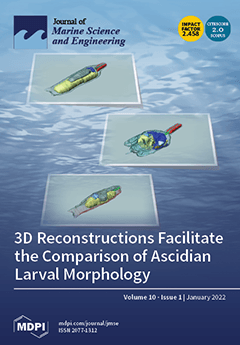
The swimming larva represent the dispersal phase of ascidians, marine invertebrates belonging to tunicates. The anatomy of larva, which reveals the structures that tunicates share with vertebrates, has been described in detail in a few species, showing different degrees of adult structure differentiation, called adultation. By 3D reconstruction, we compared the anatomy of the larva of the solitary ascidian Halocynthia roretzi, a species reared for commercial purpose, with that of two other common species: Ciona intestinalis and Botryllus schlosseri. This approach allowed us to clearly evaluate the different levels of adultation displayed by the diverse species. View this paper
  • Issues are regarded as officially published after their release is announced to the table of contents alert mailing list.
  • You may sign up for e-mail alerts to receive table of contents of newly released issues.
  • PDF is the official format for papers published in both, html and pdf forms. To view the papers in pdf format, click on the "PDF Full-text" link, and use the free Adobe Reader to open them.
Order results
Result details
Section
Select all
Export citation of selected articles as:
18 pages, 4167 KiB  
Article
Strahler Ordering Analyses on Branching Coral Canopies: Stylophora pistillata as a Case Study
by Yaniv Shmuel, Yaron Ziv and Baruch Rinkevich
J. Mar. Sci. Eng. 2022, 10(1), 121; https://doi.org/10.3390/jmse10010121 - 17 Jan 2022
Cited by 4 | Viewed by 3531
Abstract
The three-dimensional structural complexities generated by living sessile organisms, such as trees and branching corals, embrace distinct communities of dwelling organisms, many of which are adapted to specific niches within the structure. Thus, characterizing the build-up rules and the canopy compartments may clarify [...] Read more.
The three-dimensional structural complexities generated by living sessile organisms, such as trees and branching corals, embrace distinct communities of dwelling organisms, many of which are adapted to specific niches within the structure. Thus, characterizing the build-up rules and the canopy compartments may clarify small-scale biodiversity patterns and rules for canopy constituents. While biodiversity within tree canopies is usually typified by the vertical axis that is delineated by its main compartments (understory, trunk, crown), traditional studies of coral canopy dwelling species are evaluated only by viewing the whole coral head as a single homogeneous geometric structure. Here, we employ the Strahler number of a mathematical tree for the numerical measurements of the coral’s canopy complexity. We use the branching Indo-Pacific coral species Stylophora pistillata as a model case, revealing five compartments in the whole coral canopy volume (Understory, Base, Middle, Up, and Bifurcation nods). Then, the coral’s dwellers’ diel distribution patterns were quantified and analyzed. We observed 114 natal colonies, containing 32 dwelling species (11 sessile), totaling 1019 individuals during day observations, and 1359 at night (1–41 individuals/colony). Biodiversity and abundance associated with Strahler numbers, diel richness, abundance, and patterns for compartmental distributions differed significantly between day/night. These results demonstrate that the coral-canopy Strahler number is an applicable new tool for assessing canopy landscapes and canopy associated species biodiversity, including the canopy-compartmental utilization by mobile organisms during day/night and young/adult behaviors. Full article
(This article belongs to the Section Marine Biology)
Show Figures

Figure 1

Figure 1
<p>(<b>a</b>) A colony of <span class="html-italic">Stylophora pistillata</span> from Eilat’s reef (4 m depth); (<b>b</b>) A schematic illustration for Strahler order system applying on a coral canopy. Initiate branches receive the first order (1, yellow branches), and branches that are formed by joining of two branches of the same order i, receive the order i + 1; (<b>c</b>) <span class="html-italic">Stylophora pistillata</span> canopy compartments as revealed via the use of branch analyses through the Strahler order technique: Up: the outermost canopy layer, in analogy to the foliage of the tree canopy. This is the canopy peripheral volume that encloses the first Strahler order branches; Base: the canopy two highest Strahler numbers of a specific coral colony, that in analogical to trees create the canopy’s trunk; Middle: middle branches area, this is the space above the base and below the first Strahler branches, resembling the crown area of the tree’s canopy.; Understory: the space found beneath the canopy base that occupies the space between the coral’s substate plain to the parallel first canopy branches. Bifurcation: the branches node, these are the spaces surrounding the initiating axes of all branches above the base. Yellow = ‘up’ compartment; Purple = ‘middle’; Red = ‘base’; Green = ‘bifurcation’; Dark-blue = ‘understory’. Part c was extracted from a <span class="html-italic">S. pistillata</span> skeleton using Autodesk ReCap Photo and Photoshop programs.</p>
Full article ">Figure 2
<p>Canopy dweller species and total abundance within <span class="html-italic">Stylophora pistillata</span> canopies (<span class="html-italic">n</span> = 114) at day and night paired surveys. (<b>a</b>) mobile species, day time (orange) surveys, compared to night (blue); (<b>b</b>) sessile species counted in day surveys.</p>
Full article ">Figure 3
<p>Correlation between canopy volume and canopy Straler number to day/night richness and abundance. (<b>a</b>–<b>d</b>) Linear regression of Log-Log canopy volume vs. richness/abundance. Shaded areas are the standart errors for the regressions; (<b>e</b>–<b>h</b>) Canopy Strahler number vs. richness/abundance, letters indicat significantly differet groups (Permutation one way ANOVA).</p>
Full article ">Figure 4
<p>Nonmetric multidimensional scaling ordination plots for Bray–Curtis distance matrix of community dissimilarities based on 0.85 square transformation of S. pistillata dwelling species abundance data. (<b>a</b>,<b>b</b>) communities grouped by canopy size (large, medium small) at day and night time, respectively; (<b>c</b>,<b>d</b>) communities grouped by canopy Strahler order numbers (2–6) at day and night, respectively. Each canopy community sample is represented by a colored point. 2D stress values are marked for each plot.</p>
Full article ">Figure 5
<p>Proportion of three S. pistillata dwelling crustacean species according to their distribution between canopy compartments and their body-size groups during day and night censuses (left and right graphs, accordingly). (<b>a</b>,<b>b</b>) T. cymodoce; (<b>c</b>,<b>d</b>) T. digitalis; (<b>e</b>,<b>f</b>) Paguridae. Individual total observations by their size (L large, M medium, S small) are marked for each plot. Percentage was calculated according to the total abundance of each species size group for each day time census (UN) understory; (B) base; (M) middle; (B-UP) base, middle, and up; (M-UP) middle and up compartments.</p>
Full article ">Figure 6
<p>Proportion of <span class="html-italic">Stylophora pistillata</span> dwelling species according to their distribution between the canopy compartments during day and night censuses (mobile species), and for the sessile species (day surveys). (<b>a</b>) <span class="html-italic">Ophiocoma</span> sp.; (<b>b</b>) <span class="html-italic">Alpheus lottini</span>; (<b>c</b>) <span class="html-italic">Spirobranchus sp.</span>; (<b>d</b>) <span class="html-italic">Sebastapistes cyanostigma</span>; (<b>e</b>) <span class="html-italic">Paragobidon echinocephalus</span>; (<b>f</b>) <span class="html-italic">Palaemonella rotumana</span>; (<b>g</b>) <span class="html-italic">Pseudochromis olivaceus</span>; (<b>h</b>) <span class="html-italic">Ophiactis</span> sp.; (<b>i</b>) <span class="html-italic">Leiosolenus lessepsianus</span>. Percentage were calculated according to the total abundance of each species for each day time census (UN) understory, (B) base, (M) middle, (BIF) bifurcation nods; (UN-B) understory and base; (UN-M) understory, base, and middle; (UN-UP) understory, base, middle, and up; (B-M) base and middle; (B-UP) base, middle, and up; (M-UP) middle, and up compartments.</p>
Full article ">
48 pages, 8326 KiB  
Article
Investigation on Hydrodynamic Characteristics, Wave–Current Interaction and Sensitivity Analysis of Submarine Hoses Attached to a CALM Buoy
by Chiemela Victor Amaechi, Facheng Wang and Jianqiao Ye
J. Mar. Sci. Eng. 2022, 10(1), 120; https://doi.org/10.3390/jmse10010120 - 17 Jan 2022
Cited by 19 | Viewed by 3875
Abstract
There is an increase in the utilization of the floating offshore structure (FOS) called Catenary Anchor Leg Mooring (CALM) buoys and the attached marine hoses due to the increasing demand for oil and gas products. These hoses are flexible and easier to use [...] Read more.
There is an increase in the utilization of the floating offshore structure (FOS) called Catenary Anchor Leg Mooring (CALM) buoys and the attached marine hoses due to the increasing demand for oil and gas products. These hoses are flexible and easier to use but have a short service life of about 25 years. They are adaptable in ocean locations of shallow, intermediate and deep waters. In this research, a numerical model was developed using a coupling method modeled by utilizing ANSYS AQWA and Orcaflex (Orcina Ltd., Ulverston, UK) dynamic models of the CALM buoy hoses. Two cases were comparatively studied: Lazy-S and Chinese-lantern configurations, under ocean waves and current. Comparisons were also made between coupled and uncoupled models. This research presents the hydrodynamic characteristics with a sensitivity analysis on the influence of waves, current attack angle, soil gradient, soil stiffness and environmental conditions that influence the performance of marine hoses. The study comparatively looked at the configurations from dynamic amplification factors (DAF) on marine hoses. The results show that marine hoses can be easily configured to suit the designer’s need, seabed soil type, seabed topography and the profiles that are useful for manufacturers. The sensitivity analysis also shows the effect of hose parameters on its hydrodynamic behavior from the wave–current interaction (WCI). Full article
(This article belongs to the Special Issue Waves and Ocean Structures II)
Show Figures

Figure 1

Figure 1
<p>CALM Turret buoy at Apache Stag Field, Australia, Buoy during installation (Reprinted with permission from ref. [<a href="#B49-jmse-10-00120" class="html-bibr">49</a>]. Copyright 2011 Bluewater).</p>
Full article ">Figure 2
<p>Sketch of the loading and offloading operation on a CALM buoy in (<b>a</b>) Lazy-S and (<b>b</b>) Chinese-Lantern configurations, with wave forces and boundary conditions.</p>
Full article ">Figure 3
<p>The six degrees of freedom of a floating CALM buoy.</p>
Full article ">Figure 4
<p>Description of the geometry for the first concept of CALM Buoy and skirt, showing (<b>a</b>) an isometric view and (<b>b</b>) a plan view.</p>
Full article ">Figure 5
<p>Numerical model of the CALM Buoy showing (<b>a</b>) shaded and (<b>b</b>) wireframe views.</p>
Full article ">Figure 6
<p>Submarine hose profile showing the radii for inner and outer surfaces in Orcaflex.</p>
Full article ">Figure 7
<p>Schematic for the moorings on the buoy showing.</p>
Full article ">Figure 8
<p>Typical floats attached to offshore submarine hoses.</p>
Full article ">Figure 9
<p>The methodology for the sensitivity studies in the numerical modeling.</p>
Full article ">Figure 10
<p>The description of the mooring conditions for the load cases applied in the hose analysis, showing (<b>a</b>) damaged mooring line 1, (<b>b</b>) damaged mooring line 6 and (<b>c</b>) intact mooring.</p>
Full article ">Figure 11
<p>The Orcaflex line theory depicting (Adapted, courtesy of Orcina; Source: [<a href="#B127-jmse-10-00120" class="html-bibr">127</a>,<a href="#B128-jmse-10-00120" class="html-bibr">128</a>]).</p>
Full article ">Figure 12
<p>CALM buoy finite element model of (<b>a</b>) Chinese-lantern and (<b>b</b>) Lazy-S configurations.</p>
Full article ">Figure 13
<p>The JONSWAP wave spectrum for the (<b>a</b>) first sea state and (<b>b</b>) third sea state.</p>
Full article ">Figure 14
<p>Definition of wave angles on the buoy at 30<sup>o</sup> intervals showing wave heading.</p>
Full article ">Figure 15
<p>Model ocean view of the free-floating CALM buoy in ANSYS AQWA R1 2021.</p>
Full article ">Figure 16
<p>Convergence study on buoy using surge RAO (m).</p>
Full article ">Figure 17
<p>Forces on the catenary design of a mooring line.</p>
Full article ">Figure 18
<p>Validation study using the bending moment of the submarine hose, comparing the uncoupled and coupled models.</p>
Full article ">Figure 19
<p>Bending moment profile for uncoupled model showing Hose1, Hose2, three sea states and five wave angles.</p>
Full article ">Figure 20
<p>Bending moment profile for coupled model showing Hose1, Hose2, three sea states and five wave angles.</p>
Full article ">Figure 21
<p>Influence of loadings from hydrodynamics on the curvature of the submarine hose. (<b>a</b>) Hose Curvature including hose hydrodynamic load in Lazy-S config. (<b>b</b>) Hose Curvature excluding hose hydrodynamic load in Lazy-S config. (<b>c</b>) Hose Curvature including hose hydrodynamic load in Chinese-lantern config. (<b>d</b>) Hose Curvature excluding hose hydrodynamic load in Chinese-lantern config.</p>
Full article ">Figure 22
<p>Influence of loadings from hydrodynamics on the effective tension of the submarine hose. (<b>a</b>) Coupled Hose Effective Tension in Lazy-S config. (<b>b</b>) Uncoupled Hose Effective Tension in Lazy-S config. (<b>c</b>) Coupled Hose Effective Tension in Chinese-lantern config. (<b>d</b>) Uncoupled Hose Effective Tension in Chinese-lantern config.</p>
Full article ">Figure 23
<p>Curvature of submarine hose in Chinese-lantern configuration.</p>
Full article ">Figure 24
<p>Influence of hydrodynamic loads on the bending moment of the submarine hose. (<b>a</b>) Coupled model for hose bending moment in Lazy-S config. (<b>b</b>) Uncoupled hose bending moment in Lazy-S config. (<b>c</b>) Coupled hose bending moment in Chinese-lantern config. (<b>d</b>) Uncoupled hose bending moment in Chinese-lantern config.</p>
Full article ">Figure 25
<p>Influence of loadings from hydrodynamics on the <span class="html-italic">DAF<sub>Hose</sub></span> of the submarine hose. (<b>a</b>) Curvature <span class="html-italic">DAF<sub>Hose</sub></span> for the hose in Lazy-S config. (<b>b</b>) Curvature <span class="html-italic">DAF<sub>Hose</sub></span> for the hose in Chinese-lantern config. (<b>c</b>) Effective Tension <span class="html-italic">DAF<sub>Hose</sub></span> for the hose in Lasy-S config. (<b>d</b>) Effective Tension <span class="html-italic">DAF<sub>Hose</sub></span> for the hose in Chinese-lantern config. (<b>e</b>) Bending moment <span class="html-italic">DAF<sub>Hose</sub></span> for the hose in Lazy-S config. (<b>f</b>) Bending Moment <span class="html-italic">DAF<sub>Hose</sub></span> for the hose in Chinese-lantern config.</p>
Full article ">Figure 26
<p>Influence of the current velocity on the motion RAOs for the CALM buoy, showing (<b>a</b>) surge, (<b>b</b>) heave, (<b>c</b>) pitch and (<b>d</b>) yaw.</p>
Full article ">Figure 27
<p>Influence of current velocity on the first-order forces for the CALM buoy, showing (<b>a</b>) surge, (<b>b</b>) heave, (<b>c</b>) pitch and (<b>d</b>) yaw.</p>
Full article ">Figure 28
<p>Influence of surface currents (<b>a</b>,<b>b</b>) and seabed currents (<b>c</b>,<b>d</b>) on submarine hoses.</p>
Full article ">Figure 29
<p>Influence of current attack angle on bending moment (<b>a</b>,<b>b</b>), effective tension (<b>c</b>,<b>d</b>) and curvature (<b>e</b>,<b>f</b>) on hose.</p>
Full article ">Figure 30
<p>Snapshots of hose behavior at different times, <span class="html-italic">H<sub>s</sub></span> = 1.87 m, <span class="html-italic">T<sub>z</sub></span> = 4.10 s, 0° flow angle.</p>
Full article ">
17 pages, 5774 KiB  
Article
Sound Field Fluctuations in Shallow Water in the Presence of Moving Nonlinear Internal Waves
by Yanyu Jiang, Valery Grigorev and Boris Katsnelson
J. Mar. Sci. Eng. 2022, 10(1), 119; https://doi.org/10.3390/jmse10010119 - 17 Jan 2022
Cited by 9 | Viewed by 1933
Abstract
Fluctuations of sound intensity in the presence of moving nonlinear internal waves (NIWs) are studied. Prior works revealed the existence of peaks in the spectrum of these fluctuations due to mode coupling. In the given paper, the results of experiment ASIAEX 2001 are [...] Read more.
Fluctuations of sound intensity in the presence of moving nonlinear internal waves (NIWs) are studied. Prior works revealed the existence of peaks in the spectrum of these fluctuations due to mode coupling. In the given paper, the results of experiment ASIAEX 2001 are considered. Episodes are analyzed when soliton-like NIW move for ~6 h approximately along an acoustic track of length ~30 km. The depth of the ocean changes from ~350 m (position of the source) up to ~120 m near the receiver (Vertical Line Array). The source, placed near the bottom, transmitted pulses (M-sequences) with a frequency of 224 Hz. Theoretical analysis and numerical modeling show that peak frequencies in the spectrum of intensity fluctuations correspond to the most strongly interacting pairs of modes: in the given case pairs 2–3 and 3–4 and values of dominating frequencies are determined by the spatial scale of interference beating Λ of coupling modes and by the speed v of NIW. Due to the fact that in the narrowing channel velocity v decreases as well as the value of Λ, the predominant frequency as a function of time remains approximately the same. Results of modeling are in a good agreement with experimental data. Full article
Show Figures

Figure 1

Figure 1
<p>Schematic of acoustic track with a moving nonlinear internal wave (<b>left</b>), sound speed profile (<b>right</b>).</p>
Full article ">Figure 2
<p>(<b>a</b>) Temporal dependence of modal amplitudes; (<b>b</b>) spectrum of fluctuations (12) of sound intensity.</p>
Full article ">Figure 3
<p>Schematic of the experiment: (<b>a</b>) top view, (<b>b</b>) view perpendicular to the track. S224 is the source, VLA is the receiving array, Env denotes three thermistor strings. The soliton is shown with a bold dotted line.</p>
Full article ">Figure 4
<p>Temperature versus time for three thermistor strings (7 May 2001). The dotted lines show the arrival times of the soliton under consideration.</p>
Full article ">Figure 5
<p>The soliton’s velocity calculated within the framework of the two-layer model (blue line) and average velocity in two sections (black line).</p>
Full article ">Figure 6
<p>The unperturbed temperature profile (<b>a</b>), the SSP (<b>b</b>), obtained using the ship’s CTD probe, and the dependence of the speed of sound on temperature (<b>c</b>) constructed on their basis.</p>
Full article ">Figure 7
<p>Reconstruction of the sound speed field. Dashed lines denote positions of E2. Each panel shows position of NIW at the time moment indicated above the panel.</p>
Full article ">Figure 8
<p>Time as a function of the soliton’s position for different models of its speed.</p>
Full article ">Figure 9
<p>Amplitude of intensity fluctuations as a function of depth and time. The red line denotes the time moment of appearance of the soliton on the acoustic track (07:54).</p>
Full article ">Figure 10
<p>Experimental spectrogram of intensity fluctuations. Normalization: (<b>a</b>) on global maximum during all the time period (<b>b</b>) on local maximum for each moment of time. Dashed lines denote time moments of the soliton’s passing of thorough the source position (07:54) and chain E2 (11:50).</p>
Full article ">Figure 11
<p>Dominating frequency on the spectrogram using the Hamming window.</p>
Full article ">Figure 12
<p>Comparison of experiment and theory. Normalization: (<b>a</b>,<b>b</b>) to the global maximum over the whole picture; (<b>c</b>,<b>d</b>) to a local maximum on each time moment. The dashed line is the time of passage of the soliton through the chain E2 (11:50). Black lines are dependencies <math display="inline"><semantics> <mrow> <msub> <mi>F</mi> <mrow> <mi>m</mi> <mi>n</mi> </mrow> </msub> <mrow> <mo>(</mo> <mi>T</mi> <mo>)</mo> </mrow> </mrow> </semantics></math>.</p>
Full article ">Figure 13
<p>Modal amplitudes <math display="inline"><semantics> <mrow> <msub> <mi>C</mi> <mi>m</mi> </msub> <mrow> <mo>(</mo> <mi>r</mi> <mo>)</mo> </mrow> </mrow> </semantics></math> for the waveguide without the soliton. In area of 25 km there is area of steep slope between shallow and deep parts of acoustic track.</p>
Full article ">
11 pages, 30663 KiB  
Article
Methods and Proposals for Solutions in the Applicability of a Software-Defined Radio in Maritime Communication
by Miroslav Bistrović and Domagoj Komorčec
J. Mar. Sci. Eng. 2022, 10(1), 118; https://doi.org/10.3390/jmse10010118 - 17 Jan 2022
Cited by 1 | Viewed by 2280
Abstract
Ship communication systems are defined in one part as GMDSS, while the other part consists of systems with secondary importance in safety communications. Each of these devices and systems makes an independent or separate system that works in a specific frequency range and [...] Read more.
Ship communication systems are defined in one part as GMDSS, while the other part consists of systems with secondary importance in safety communications. Each of these devices and systems makes an independent or separate system that works in a specific frequency range and is, at some level, connected to other communication systems. A step forward regarding frequency range and level of networking can be achieved with the application of a software-defined radio. This paper examines a variety of GMDSS communication equipment in terms of technical discrepancy and frequency range. Furthermore, the software-defined radio and SDR configuration development are described according to their theoretical feasibility in the maritime domain. The paper proposes the concept of SDR-based communication systems quite different from conventional maritime communication systems. This approach, conducted in phases, would in turn ease the upgrading, enable flexibility and inter-operation, prolong system life cycle and integrate different maritime communication systems and devices. The proposed concept aims to develop a centralized communication system to incorporate the ship’s communication devices into one common ship communication system. Full article
(This article belongs to the Section Ocean Engineering)
Show Figures

Figure 1

Figure 1
<p>GMDSS communication used on a ship.</p>
Full article ">Figure 2
<p>Block scheme of a typical radio receiver.</p>
Full article ">Figure 3
<p>Goals of the SDR system implementation.</p>
Full article ">Figure 4
<p>A generic hardware configuration of SDR.</p>
Full article ">Figure 5
<p>Comparison of conventional and digital RF architecture.</p>
Full article ">Figure 6
<p>Types of MIMO approaches in the design of the antenna.</p>
Full article ">Figure 7
<p>Model of the maritime communications system based on the SDR approach.</p>
Full article ">Figure 8
<p>Development phases of SDR for the needs of maritime communications.</p>
Full article ">
19 pages, 9629 KiB  
Article
Modular Approach in the Design of Small Passenger Vessels for Mediterranean
by Nikola Vladimir, Andro Bakica, Maja Perčić and Ivana Jovanović
J. Mar. Sci. Eng. 2022, 10(1), 117; https://doi.org/10.3390/jmse10010117 - 17 Jan 2022
Cited by 3 | Viewed by 2855
Abstract
This paper deals with the modular concept in the design of small passenger vessels for the Mediterranean, where the ship is assembled from three virtual modules (hull, power system and superstructure), enabling different vessel characteristics (speed, capacity, environmental performance, habitability, etc.). A set [...] Read more.
This paper deals with the modular concept in the design of small passenger vessels for the Mediterranean, where the ship is assembled from three virtual modules (hull, power system and superstructure), enabling different vessel characteristics (speed, capacity, environmental performance, habitability, etc.). A set of predefined modules is established based on the investigation of market needs, where the IHS Fairplay database is taken as a reference for ship particulars and power needs, while the set of environmental regulation scenarios and requirements on ship habitability are taken as relevant for the design of ship power systems and superstructure modules, respectively. For the selected hull, a series of computations have been conducted to obtain their resistance and power needs which are further satisfied in the above-described manner. Within the illustrative example, a small passenger vessel with a capacity of 250 passengers is considered, with a detailed description of relevant modules that fit future design requirement scenarios. This approach is aimed at small-scale shipyards with limited research capabilities, who can quickly obtain the preliminary design of the vessel which can be further optimized to the final solution. Full article
(This article belongs to the Section Ocean Engineering)
Show Figures

Figure 1

Figure 1
<p>Ship design and exploitation over time [<a href="#B3-jmse-10-00117" class="html-bibr">3</a>,<a href="#B17-jmse-10-00117" class="html-bibr">17</a>] (reproduced from [<a href="#B3-jmse-10-00117" class="html-bibr">3</a>] with permission of the Society of Naval Architects of Korea (SNAK), 2021).</p>
Full article ">Figure 2
<p>Methodology scheme.</p>
Full article ">Figure 3
<p>(<b>a</b>) Deadweight vs. Length overall, (<b>b</b>) Deadweight vs. Draft, (<b>c</b>) Deadweight vs. Beam, (<b>d</b>) Deadweight vs. Power.</p>
Full article ">Figure 4
<p>(<b>a</b>) Deadweight vs. Number of passengers, (<b>b</b>) Length overall vs. Number of passengers.</p>
Full article ">Figure 5
<p>Type of propulsors in the considered passenger vessels.</p>
Full article ">Figure 6
<p>The IMO strategy for the reduction of GHG emissions (reproduced from [<a href="#B31-jmse-10-00117" class="html-bibr">31</a>] with permission of Det Norske Veritas (DNV), 2022).</p>
Full article ">Figure 7
<p>Decarbonization measures.</p>
Full article ">Figure 8
<p>Main noise sources onboard [<a href="#B35-jmse-10-00117" class="html-bibr">35</a>].</p>
Full article ">Figure 9
<p>Source-Path-Receiver model.</p>
Full article ">Figure 10
<p>Hull modules are used within the proposed design procedure (fore, mid and stern modules).</p>
Full article ">Figure 11
<p>(<b>a</b>) Two adjacent compartments with noise source and receiver, (<b>b</b>) insulated bulkhead between passenger spaces.</p>
Full article ">Figure 12
<p>Noise reduction potential of different materials and specific prices.</p>
Full article ">Figure 13
<p>Comparative analysis of prices for different insulation materials.</p>
Full article ">Figure 14
<p>Noise levels at the receivers for different insulation materials.</p>
Full article ">Figure 15
<p>Vibratory response at passenger spaces depending on ship transfer functions and shifting to higher comfort level.</p>
Full article ">Figure 16
<p>Computational mesh and free surface at ship design speed (V = 14 kn).</p>
Full article ">Figure 17
<p>Resistance curve computed in CFD.</p>
Full article ">Figure 18
<p>Righting lever curve (GZ) for design draft.</p>
Full article ">Figure 19
<p>A comparison of the LCA and LCCA of alternative fuels.</p>
Full article ">Figure 20
<p>Typical results of noise prediction for ship compartments.</p>
Full article ">
20 pages, 4786 KiB  
Article
Research on the Water Ridge and Slamming Characteristics of a Semisubmersible Platform under Towing Conditions
by Fali Huo, Changdong Wei, Chenyang Zhu, Zhaojun Yuan and Sheng Xu
J. Mar. Sci. Eng. 2022, 10(1), 116; https://doi.org/10.3390/jmse10010116 - 15 Jan 2022
Cited by 1 | Viewed by 1813
Abstract
During the towing of semisubmersible platforms, waves impact and superpose in front of the platform to form a ridge shaped “water ridge”, which protrudes near the platform and produces a large slamming pressure. The water ridges occur frequently in the towing conditions of [...] Read more.
During the towing of semisubmersible platforms, waves impact and superpose in front of the platform to form a ridge shaped “water ridge”, which protrudes near the platform and produces a large slamming pressure. The water ridges occur frequently in the towing conditions of semisubmersible platforms. The wave–slamming on the braces and columns of platform is aggravated due to the water ridges, particularly in rough sea conditions. The effect of water ridges is usually ignored in slamming pressure analysis, which is used to check the structural strengths of the braces and columns. In this paper, the characteristics of the water ridge at the braces of a semisubmersible platform are studied by experimental tests and numerical simulations. In addition, the sensitivity of the water ridge to the wave height and period is studied. The numerical simulations are conducted by a Computational Fluid Dynamics (CFD) method, and their accuracy is validated based on experimental tests. The characteristics of the water ridge and slamming pressure on the braces and columns are studied in different wave conditions based on the validated numerical model. It is found that the wave extrusion is the main reason of water ridge. The wave–slamming pressure caused by the water ridge has an approximately linear increase with the wave height and is sensitive to the wave period. With the increase of the wave period, the wave–slamming pressure on the brace and column of the platform increases first and then decreases. The maximum wave–slamming pressure is found when the wave period is 10 s and the slamming pressure reduces rapidly with an increase of wave period. Full article
(This article belongs to the Special Issue Ship Motions and Wave Loads)
Show Figures

Figure 1

Figure 1
<p>Semisubmersible platform. (<b>a</b>) Numerical platform configuration. (<b>b</b>) Test platform model.</p>
Full article ">Figure 2
<p>Distribution of the monitoring points.</p>
Full article ">Figure 3
<p>Numerical wave tank.</p>
Full article ">Figure 4
<p>Computational domain grid and overlapping area grid. (<b>a</b>) Computational domain grid. (<b>b</b>) Overlapping area grid.</p>
Full article ">Figure 5
<p>Pitch decay cures of the platform under 2 degrees of inclination.</p>
Full article ">Figure 6
<p>Comparison between theoretical numerical and waveform. (<b>a</b>) 4 m from the calculation domain entrance. (<b>b</b>) 12 m from the calculation domain entrance.</p>
Full article ">Figure 7
<p>Installation position of the wave gauge.</p>
Full article ">Figure 8
<p>Wave time history of three foundation sizes. (<b>a</b>) Foundation size: 1 m. (<b>b</b>) Foundation size: 2 m. (<b>c</b>) Foundation size: 3 m.</p>
Full article ">Figure 9
<p>Comparison of points A4 A7 and B3 wave pressure under the same wave conditions. (<b>a</b>) The monitoring points of A4. (<b>b</b>) The monitoring points of A7. (<b>c</b>) The monitoring points of B3.</p>
Full article ">Figure 10
<p>Comparison of points A7 wave pressure under the C12 working condition. (<b>a</b>) Monitoring points of A7. (<b>b</b>) Monitoring points of B3.</p>
Full article ">Figure 11
<p>Water ridge phenomenon of the wave during the towing test. (<b>a</b>) Entering the water. (<b>b</b>) Exiting the water.</p>
Full article ">Figure 12
<p>Water ridge in front of the column. (<b>a</b>) Water ridge. (<b>b</b>) Wave run–up.</p>
Full article ">Figure 13
<p>Water ridge under the brace. (<b>a</b>) First water ridge. (<b>b</b>) Second water ridge.</p>
Full article ">Figure 14
<p>Wave pressure and wave run–up under the brace. (<b>a</b>) Time history curves of the wave pressure at different wave heights. (<b>b</b>) Time history curves of the wave pressure and wave run–up in the C5 case. (<b>c</b>) Time history curves of the wave pressure and wave run–up in the C11 case.</p>
Full article ">Figure 15
<p>Variation of wave pressure with wave height. (<b>a</b>) Wave pressure at B1. (<b>b</b>) Wave pressure at A7.</p>
Full article ">Figure 16
<p>Wave pressure and wave run–up under the brace. (<b>a</b>)Time history curves of the wave pressure at different wave periods. (<b>b</b>) Time history curves of the wave pressure and wave run–up.</p>
Full article ">Figure 17
<p>Variation of wave pressure with wave period. (<b>a</b>) Wave pressure on the column. (<b>b</b>) Wave pressure on the brace.</p>
Full article ">
24 pages, 10247 KiB  
Article
Research on the Matching Characteristics of the Impellers and Guide Vanes of Seawater Desalination Pumps with High Capacity and Pressure
by Wei Li, Mingjiang Liu, Leilei Ji, Yulu Wang, Muhammad Awais, Jingning Hu and Xiaoyan Ye
J. Mar. Sci. Eng. 2022, 10(1), 115; https://doi.org/10.3390/jmse10010115 - 15 Jan 2022
Cited by 2 | Viewed by 4275
Abstract
This paper presents the matching characteristics of impellers and guide vanes of high capacity and pressure seawater desalination pumps by using computational fluid dynamics (CFD). The single-stage pump is numerically calculated, and its external characteristics are consistent with the test results of model [...] Read more.
This paper presents the matching characteristics of impellers and guide vanes of high capacity and pressure seawater desalination pumps by using computational fluid dynamics (CFD). The single-stage pump is numerically calculated, and its external characteristics are consistent with the test results of model pump. Taking this scheme as a prototype, the research is carried out from three aspects: (i) the impeller blade outlet width; (ii) the number of impeller and guide vane blades; and (iii) the area ratio of impeller outlet to guide vane inlet. The results indicate that the blade outlet width significantly affects the pump head and efficiency. Appropriately increasing the number of guide vane blades or changing the number of impeller blades can improve efficiency and expand the high-efficiency area. Additionally, increasing the throat area of the guide vane has the opposite effect on the large flow and small flow area of the pump. An optimized hydraulic model design scheme is obtained. Full article
(This article belongs to the Section Ocean Engineering)
Show Figures

Figure 1

Figure 1
<p>Structure diagram of single-stage pump model.</p>
Full article ">Figure 2
<p>Three-dimensional modeling of main overflow components. (<b>a</b>) Guide vane entity, (<b>b</b>) Guide vane water body, (<b>c</b>) Impeller entity, (<b>d</b>) Impeller water body.</p>
Full article ">Figure 3
<p>Fluid computing domain of single-stage model pump.</p>
Full article ">Figure 4
<p>Meshing of main flow through components. (<b>a</b>) Impeller, (<b>b</b>) Guide vane, (<b>c</b>) Front pump chamber, (<b>d</b>) Rear pump chamber, (<b>e</b>) Outlet section.</p>
Full article ">Figure 5
<p>Assembly meshing in the fluid computing domain.</p>
Full article ">Figure 6
<p>Schematic diagram of the test bench.</p>
Full article ">Figure 7
<p>Model pump installation illustration.</p>
Full article ">Figure 8
<p>Comparison of external characteristics of numerical simulation and test.</p>
Full article ">Figure 9
<p>Four groups of impellers with different blade outlet widths. (<b>a</b>) <span class="html-italic">b</span><sub>2</sub> = 24 mm, (<b>b</b>) <span class="html-italic">b</span><sub>2</sub> = 26 mm, (<b>c</b>) <span class="html-italic">b</span><sub>2</sub> = 28 mm, (<b>d</b>) <span class="html-italic">b</span><sub>2</sub> = 30 mm.</p>
Full article ">Figure 10
<p>External characteristic curve of different blade outlet widths. (<b>a</b>) <span class="html-italic">Q-H</span>, (<b>b</b>) <span class="html-italic">Q-η</span>.</p>
Full article ">Figure 11
<p>Pressure distribution of impeller and guide vane with different <span class="html-italic">b</span><sub>2</sub> value. (<b>a</b>) <span class="html-italic">b</span><sub>2</sub> = 24 mm, (<b>b</b>) <span class="html-italic">b</span><sub>2</sub> = 26 mm, (<b>c</b>) <span class="html-italic">b</span><sub>2</sub> = 28 mm, (<b>d</b>) <span class="html-italic">b</span><sub>2</sub> = 30 mm.</p>
Full article ">Figure 11 Cont.
<p>Pressure distribution of impeller and guide vane with different <span class="html-italic">b</span><sub>2</sub> value. (<b>a</b>) <span class="html-italic">b</span><sub>2</sub> = 24 mm, (<b>b</b>) <span class="html-italic">b</span><sub>2</sub> = 26 mm, (<b>c</b>) <span class="html-italic">b</span><sub>2</sub> = 28 mm, (<b>d</b>) <span class="html-italic">b</span><sub>2</sub> = 30 mm.</p>
Full article ">Figure 12
<p>Velocity distribution of impellers and guide vanes with different <span class="html-italic">b</span><sub>2</sub> values. (<b>a</b>) <span class="html-italic">b</span><sub>2</sub> = 24 mm, (<b>b</b>) <span class="html-italic">b</span><sub>2</sub> = 26 mm, (<b>c</b>) <span class="html-italic">b</span><sub>2</sub> = 28 mm, (<b>d</b>) <span class="html-italic">b</span><sub>2</sub> = 30 mm.</p>
Full article ">Figure 13
<p>Three-dimensional modeling of impeller and guide vane. (<b>a</b>) 6-blade impeller, (<b>b</b>) 7-blade impeller, (<b>c</b>) 8-blade impeller, (<b>d</b>) 5-blade guide vane, (<b>e</b>) 7-blade guide vane, (<b>f</b>) 9-blade guide vane.</p>
Full article ">Figure 13 Cont.
<p>Three-dimensional modeling of impeller and guide vane. (<b>a</b>) 6-blade impeller, (<b>b</b>) 7-blade impeller, (<b>c</b>) 8-blade impeller, (<b>d</b>) 5-blade guide vane, (<b>e</b>) 7-blade guide vane, (<b>f</b>) 9-blade guide vane.</p>
Full article ">Figure 14
<p>Characteristic curves of various schemes when the impeller blade number is 6. (<b>a</b>) <span class="html-italic">Q-H</span>, (<b>b</b>) <span class="html-italic">Q-η</span>.</p>
Full article ">Figure 15
<p>Characteristic curves of various schemes when the impeller blade number is 7. (<b>a</b>) <span class="html-italic">Q-H</span>, (<b>b</b>) <span class="html-italic">Q-η</span>.</p>
Full article ">Figure 16
<p>Characteristic curves of various schemes when the impeller blade number is 8. (<b>a</b>) <span class="html-italic">Q-H</span>, (<b>b</b>) <span class="html-italic">Q-η</span>.</p>
Full article ">Figure 17
<p>Characteristic curves of different schemes when the guide vane number is 5. (<b>a</b>) <span class="html-italic">Q-H</span>, (<b>b</b>) <span class="html-italic">Q-η</span>.</p>
Full article ">Figure 18
<p>Characteristic curves of different schemes when the guide vane number is 7. (<b>a</b>) <span class="html-italic">Q-H</span>, (<b>b</b>) <span class="html-italic">Q-η</span>.</p>
Full article ">Figure 19
<p>Characteristic curves of different schemes when the guide vane number is 9. (<b>a</b>) <span class="html-italic">Q-H</span>, (<b>b</b>) <span class="html-italic">Q-η</span>.</p>
Full article ">Figure 20
<p>Pressure distribution of different guide vane schemes under the 8-blade impeller. (<b>a</b>) 5-blade guide vane, (<b>b</b>) 7-blade guide vane, (<b>c</b>) 9-blade guide vane.</p>
Full article ">Figure 21
<p>Velocity distribution of different guide vane schemes under the 8-blade impeller. (<b>a</b>) 5-blade impeller, (<b>b</b>) 7-blade impeller, (<b>c</b>) 9-blade impeller.</p>
Full article ">Figure 22
<p>Pressure distribution of different impeller blade numbers under the 7-blade guide vane. (<b>a</b>) 6-blade impeller, (<b>b</b>) 7-blade impeller, (<b>c</b>) 8-blade impeller.</p>
Full article ">Figure 23
<p>Velocity distribution of different impeller blade numbers under the 7-blade guide vane. (<b>a</b>) 6-blade impeller, (<b>b</b>) 7-blade impeller, (<b>c</b>) 8-blade impeller.</p>
Full article ">Figure 24
<p>Three-dimensional modeling of the four guide vanes. (<b>a</b>) Guide vane 1, (<b>b</b>) Guide vane 2, (<b>c</b>) Guide vane 3, (<b>d</b>) Guide vane 4.</p>
Full article ">Figure 25
<p>External characteristic curve of the different throat area schemes. (<b>a</b>) <span class="html-italic">Q-H</span>, (<b>b</b>) <span class="html-italic">Q-η</span>.</p>
Full article ">Figure 26
<p>Turbulence kinetic energy distribution of M1 scheme under different flow conditions. (<b>a</b>) 0.8<span class="html-italic">Q</span><sub>des</sub>, (<b>b</b>) 1.0<span class="html-italic">Q</span><sub>des</sub>, (<b>c</b>) 1.2<span class="html-italic">Q</span><sub>des</sub>.</p>
Full article ">Figure 27
<p>Turbulence kinetic energy distribution of M3 scheme under different flow conditions. (<b>a</b>) 0.8<span class="html-italic">Q</span><sub>des</sub>, (<b>b</b>) 1.0<span class="html-italic">Q</span><sub>des</sub>, (<b>c</b>) 1.2<span class="html-italic">Q</span><sub>des</sub>.</p>
Full article ">
13 pages, 1652 KiB  
Article
The Isolation of Vibrio crassostreae and V. cyclitrophicus in Lesser-Spotted Dogfish (Scyliorhinus canicula) Juveniles Reared in a Public Aquarium
by Mattia Tomasoni, Giuseppe Esposito, Davide Mugetti, Paolo Pastorino, Nadia Stoppani, Vasco Menconi, Flavio Gagliardi, Ilaria Corrias, Angela Pira, Pier Luigi Acutis, Alessandro Dondo, Marino Prearo and Silvia Colussi
J. Mar. Sci. Eng. 2022, 10(1), 114; https://doi.org/10.3390/jmse10010114 - 15 Jan 2022
Cited by 5 | Viewed by 2679
Abstract
The genus Vibrio currently contains 147 recognized species widely distributed, including pathogens for aquatic organisms. Vibrio infections in elasmobranchs are poorly reported, often with identifications as Vibrio sp. and without detailed diagnostic insights. The purpose of this paper is the description of the [...] Read more.
The genus Vibrio currently contains 147 recognized species widely distributed, including pathogens for aquatic organisms. Vibrio infections in elasmobranchs are poorly reported, often with identifications as Vibrio sp. and without detailed diagnostic insights. The purpose of this paper is the description of the isolation and identification process of Vibrio spp. following a mortality event of Scyliorhinus canicula juvenile reared in an Italian public aquarium. Following investigations aimed at excluding the presence of different pathogens of marine fish species (parasites, bacteria, Betanodavirus), several colonies were isolated and subjected to species identification using the available diagnostic techniques (a biochemical test, MALDI-TOF MS, and biomolecular analysis). Discrepancies were observed among the methods; the limits of biochemistry as a unique tool for Vibrio species determination were detected through statistical analysis. The use of the rpoB gene, as a diagnostic tool, allowed the identification of the isolates as V. crassostreae and V. cyclotrophicus. Although the pathogenic role of these microorganisms in lesser-spotted dogfish juveniles has not been demonstrated, and the presence of further pathogens cannot be excluded, this study allowed the isolation of two Vibrio species in less-studied aquatic organisms, highlighting the weaknesses and strengths of the different diagnostic methods applied. Full article
(This article belongs to the Special Issue Microbial Diseases of Marine Organisms)
Show Figures

Figure 1

Figure 1
<p>Specimens of lesser-spotted dogfish (<span class="html-italic">Scyliorhinus canicula</span>) analyzed during this survey.</p>
Full article ">Figure 2
<p>Biochemical features of isolates (API<sup>®</sup> 20E). ONPG: test for β-galactosidase enzyme by hydrolysis of the substrate o-nitrophenyl-b-D-galactopyranoside; ADH, decarboxylation of the amino acid arginine by arginine dihydrolase; LDC, decarboxylation of the amino acid lysine by lysine decarboxylase; ODC, decarboxylation of the amino acid ornithine by ornithine decarboxylase; CIT, utilization of citrate as only carbon source; H<sub>2</sub>S, production of hydrogen sulfide; URE, test for the enzyme urease; TDA, tryptophan deaminase; detection of the enzyme tryptophan deaminase: reagent, ferric chloride; IND: indole test production of indole from tryptophan by the enzyme tryptophanase. Reagent–indole is detected by addition of Kovac’s reagent; VP, the Voges–Proskauer test for the detection of acetoin (acetyl methylcarbinol) produced by fermentation of glucose by bacteria utilizing the butylene glycol pathway; GEL, test for the production of the enzyme gelatinase, which liquefies gelatin; GLU, fermentation of glucose (hexose sugar); MAN, fermentation of mannose (hexose sugar); INO, fermentation of inositol (cyclic polyalcohol); SOR, fermentation of sorbitol (alcohol sugar); RHA, fermentation of rhamnose (methyl pentose sugar); SAC, fermentation of sucrose (disaccharide); MEL, fermentation of melibiose (disaccharide); AMY, fermentation of amygdalin (glycoside); ARA, fermentation of arabinose (pentose sugar). In the last two columns, there is the API identifier and the real identifier provided by the molecular analysis.</p>
Full article ">Figure 3
<p>Phylogenetic relationship among <span class="html-italic">Vibrio</span> species isolated from lesser-spotted dogfish and different <span class="html-italic">Vibrio</span> species. Phylogenetic tree was constructed using MEGAX and neighbor-joining method. A bootstrap test of 1000 replicates was performed; the bootstrap condensed tree, using a cut-off value of 50% is shown. The sequences with “G” displayed after the scientific name derived from a deposited genome.</p>
Full article ">Figure 4
<p>Principal component analysis of biochemical features of <span class="html-italic">Vibrio</span> spp. strains based on phenotypic species identification (API<sup>®</sup> 20E test). The blue cluster contains most of the strains that were similar in biochemical features (<span class="html-italic">Vibrio celticus</span>, <span class="html-italic">V. gigantis</span>, and <span class="html-italic">V. gallicus</span>). The red cluster contains <span class="html-italic">V. fluvialis</span>, whereas the green cluster contains <span class="html-italic">Aeromonas hydrophila</span> and <span class="html-italic">V. splendidus</span>. Confidence ellipses (95%) plot convex hull values of each cluster.</p>
Full article ">Figure 5
<p>Principal component analysis of biochemical features of <span class="html-italic">Vibrio</span> spp. strains based on molecular species identification. The red cluster contains most of the strains that belonged to <span class="html-italic">V. crassostreae</span>, whereas the blue cluster contains <span class="html-italic">V. cyclitrophicus</span>. Confidence ellipses (95%) plot convex hull values of each cluster.</p>
Full article ">
26 pages, 12759 KiB  
Article
CFD Simulation and Experimental Study on Coupled Motion Response of Ship with Tank in Beam Waves
by Tao He, Dakui Feng, Liwei Liu, Xianzhou Wang and Hua Jiang
J. Mar. Sci. Eng. 2022, 10(1), 113; https://doi.org/10.3390/jmse10010113 - 14 Jan 2022
Cited by 14 | Viewed by 2643
Abstract
Tank sloshing is widely present in many engineering fields, especially in the field of marine. Due to the trend of large-scale liquid cargo ships, it is of great significance to study the coupled motion response of ships with tanks in beam waves. In [...] Read more.
Tank sloshing is widely present in many engineering fields, especially in the field of marine. Due to the trend of large-scale liquid cargo ships, it is of great significance to study the coupled motion response of ships with tanks in beam waves. In this study, the CFD (Computational Fluid Dynamics) method and experiments are used to study the response of a ship with/without a tank in beam waves. All the computations are performed by an in-house CFD solver, which is used to solve RANS (Reynold Average Navier-Stokes) equations coupled with six degrees-of-freedom solid-body motion equations. The Level Set Method is used to solve the free surface. Verification work on the grid number and time step size has been conducted. The simulation results agree with the experimental results well, which shows that the numerical method is accurate enough. In this paper, several different working conditions are set up, and the effects of the liquid height in the tank, the size of the tank and the wavelength ratio of the incident wave on the ship’s motion are studied. The results show the effect of tank sloshing on the ship’s motion in different working conditions. Full article
(This article belongs to the Special Issue Ship Motions and Wave Loads)
Show Figures

Figure 1

Figure 1
<p>Model size parameters.</p>
Full article ">Figure 2
<p>Experimental model and wave making (<b>a</b>) The experimental model; (<b>b</b>) The scene of making waves.</p>
Full article ">Figure 3
<p>The layout of the pressure sensor for the side bulkhead of the tank (<b>a</b>) The pressure sensor and the tank; (<b>b</b>) The layout of the pressure sensor.</p>
Full article ">Figure 4
<p>Measuring equipment in the experiment (<b>a</b>) The Angle measuring instrument; (<b>b</b>) The data acquisition instrument; (<b>c</b>) The pressure sensor.</p>
Full article ">Figure 4 Cont.
<p>Measuring equipment in the experiment (<b>a</b>) The Angle measuring instrument; (<b>b</b>) The data acquisition instrument; (<b>c</b>) The pressure sensor.</p>
Full article ">Figure 5
<p>Coordinate system.</p>
Full article ">Figure 6
<p>Surface grid of the ship.</p>
Full article ">Figure 7
<p>Comparison of the grid before and after overset.</p>
Full article ">Figure 8
<p>Computational domain and boundary conditions.</p>
Full article ">Figure 9
<p>Time histories of <math display="inline"><semantics> <mover accent="true"> <mi>θ</mi> <mo>˜</mo> </mover> </semantics></math> of the ship obtained on grids 1, 2 and 3.</p>
Full article ">Figure 10
<p>Time histories of <math display="inline"><semantics> <mover accent="true"> <mi>θ</mi> <mo>˜</mo> </mover> </semantics></math> of the ship obtained on grid 2 from simulations with three different time steps.</p>
Full article ">Figure 11
<p>Comparison of the roll angle of ship with tank between CFD and EFD at a wavelength ratio of 1.334 and a tank length of 1.17 m.</p>
Full article ">Figure 12
<p>For the ship in beam waves, comparative roll amplitudes by CFD and EFD without accounting for sloshing in tanks.</p>
Full article ">Figure 13
<p>For the ship in beam waves, comparative roll amplitudes of the ship obtained from numerical simulations and experiment with and without a tank.</p>
Full article ">Figure 14
<p>Roll moment of the ship and tank when the wavelength ratio is 0.787 (<b>a</b>) The height of liquid in the tank is 0.1 m; (<b>b</b>) The height of liquid in the tank is 0.2 m.</p>
Full article ">Figure 15
<p>Rolling moment of the ship and tank (the height of liquid in the tank is 0.1 m) when the wavelength ratio is 0.463.</p>
Full article ">Figure 16
<p>The pressure amplitude of two points on the bulkhead.</p>
Full article ">Figure 17
<p>The heave amplitude of the ship.</p>
Full article ">Figure 18
<p>For the ship in beam waves at <math display="inline"><semantics> <mrow> <mi>λ</mi> <mo>/</mo> <mi>L</mi> <mo>=</mo> <mn>0.787</mn> </mrow> </semantics></math>, time histories of the force in z direction.</p>
Full article ">Figure 19
<p>The wave pattern in different time.</p>
Full article ">Figure 20
<p>For the ship in beam waves at λ/L = 0.787 with the height of liquid in the tank at 0.1 m, wave-induced ship positions and sloshing-induced surface elevations inside the tank at time steps of t = 0, t = 1/4 × T, t = 1/2 × T and t = 3/4 × T.</p>
Full article ">Figure 21
<p>For the ship in beam waves at λ/L = 0.787 with the height of the liquid in the tank at 0.2 m, wave-induced ship positions and sloshing-induced surface elevations inside the tank at time steps of t = 0, t = 1/4 × T, t = 1/2 × T and t = 3/4 × T.</p>
Full article ">Figure 22
<p>For the ship in beam waves at λ/L = 0.787 with the height of the liquid in the tank at 0.3 m, wave-induced ship positions and sloshing-induced surface elevations inside the tank at time steps of t = 0, t = 1/4 × T, t = 1/2 × T, and t = 3/4 × T.</p>
Full article ">Figure 23
<p>For the ship in beam waves, comparative roll amplitudes of the ship obtained from numerical simulations and experiment with and without tank.</p>
Full article ">Figure 24
<p>The heave amplitude of the ship.</p>
Full article ">Figure 25
<p>The amplitude of transverse force on the tank (Case 1: The size of the tank is 0.57 × 0.57 × 0.5 m, and the height of liquid in the tank is 0.1 m; Case 2: The size of the tank is 0.57 × 0.57 × 0.5 m, and the height of liquid in the tank is 0.2 m; Case 3: The size of the tank is 1.17 × 0.57 × 0.5 m, and the height of liquid in the tank is 0.1 m).</p>
Full article ">
19 pages, 1661 KiB  
Review
Anomaly Detection in Maritime AIS Tracks: A Review of Recent Approaches
by Konrad Wolsing, Linus Roepert, Jan Bauer and Klaus Wehrle
J. Mar. Sci. Eng. 2022, 10(1), 112; https://doi.org/10.3390/jmse10010112 - 14 Jan 2022
Cited by 52 | Viewed by 10700
Abstract
The automatic identification system (AIS) was introduced in the maritime domain to increase the safety of sea traffic. AIS messages are transmitted as broadcasts to nearby ships and contain, among others, information about the identification, position, speed, and course of the sending vessels. [...] Read more.
The automatic identification system (AIS) was introduced in the maritime domain to increase the safety of sea traffic. AIS messages are transmitted as broadcasts to nearby ships and contain, among others, information about the identification, position, speed, and course of the sending vessels. AIS can thus serve as a tool to avoid collisions and increase onboard situational awareness. In recent years, AIS has been utilized in more and more applications since it enables worldwide surveillance of virtually any larger vessel and has the potential to greatly support vessel traffic services and collision risk assessment. Anomalies in AIS tracks can indicate events that are relevant in terms of safety and also security. With a plethora of accessible AIS data nowadays, there is a growing need for the automatic detection of anomalous AIS data. In this paper, we survey 44 research articles on anomaly detection of maritime AIS tracks. We identify the tackled AIS anomaly types, assess their potential use cases, and closely examine the landscape of recent AIS anomaly research as well as their limitations. Full article
(This article belongs to the Special Issue Risk Assessment and Traffic Behaviour Evaluation of Ships)
Show Figures

Figure 1

Figure 1
<p>The usual shipping lanes and common patterns are directly accessible in the visualization of AIS messages, exemplarily shown for the Gulf of Mexico (first four days of June 2020). The historic AIS data is made publicly available by the NOAA Office for Costal Management (AIS data was obtained by <a href="https://coast.noaa.gov/htdata/CMSP/AISDataHandler/2020/index.html" target="_blank">https://coast.noaa.gov/htdata/CMSP/AISDataHandler/2020/index.html</a>, accessed on 3 December 2021. Note that the central area with sparse AIS data might be explainable by the range of AIS transceivers and the providers’ reception capabilities).</p>
Full article ">Figure 2
<p>These general five AIS anomaly types, derived by Lane et al. [<a href="#B33-jmse-10-00112" class="html-bibr">33</a>], are used in the survey to classify the capabilities of published anomaly detectors. The arrows and data marked in orange in each figure indicate a potential deviation from the normally expected patterns.</p>
Full article ">Figure 3
<p>Classification of the underlying anomaly detection methods. Besides frameworks or miscellaneous approaches, most works can be grouped into one of the the major groups: machine-learning, stochastic, or geometry approaches.</p>
Full article ">
13 pages, 4708 KiB  
Article
Pore-Scale Investigation of the Electrical Property and Saturation Exponent of Archie’s Law in Hydrate-Bearing Sediments
by Jinhuan Zhao, Changling Liu, Chengfeng Li, Yongchao Zhang, Qingtao Bu, Nengyou Wu, Yang Liu and Qiang Chen
J. Mar. Sci. Eng. 2022, 10(1), 111; https://doi.org/10.3390/jmse10010111 - 14 Jan 2022
Cited by 16 | Viewed by 2013
Abstract
Characterizing the electrical property of hydrate-bearing sediments is essential for hydrate reservoir identification and saturation evaluation. As the major contributor to electrical conductivity, pore water is a key factor in characterizing the electrical properties of hydrate-bearing sediments. The objective of this study is [...] Read more.
Characterizing the electrical property of hydrate-bearing sediments is essential for hydrate reservoir identification and saturation evaluation. As the major contributor to electrical conductivity, pore water is a key factor in characterizing the electrical properties of hydrate-bearing sediments. The objective of this study is to clarify the effect of hydrates on pore water and the relationship between pore water characteristics and the saturation exponent of Archie’s law in hydrate-bearing sediments. A combination of X-ray computed tomography and resistivity measurement technology is used to derive the three-dimensional spatial structure and resistivity of hydrate-bearing sediments simultaneously, which is helpful to characterize pore water and investigate the saturation exponent of Archie’s law at the micro-scale. The results show that the resistivity of hydrate-bearing sediments is controlled by changes in pore water distribution and connectivity caused by hydrate formation. With the increase of hydrate saturation, pore water connectivity decreases, but the average coordination number and tortuosity increase due to much smaller and more tortuous throats of pore water divided by hydrate particles. It is also found that the saturation exponent of Archie’s law is controlled by the distribution and connectivity of pore water. As the parameters of connected pore water (e.g., porosity, water saturation) decrease, the saturation exponent decreases. At a low hydrate-saturation stage, the saturation exponent of Archie’s law changes obviously due to the complicated pore structure of hydrate-bearing sediments. A new logarithmic relationship between the saturation exponent of Archie’s law and the tortuosity of pore water is proposed which helps to calculate field hydrate saturation using resistivity logging data. Full article
Show Figures

Figure 1

Figure 1
<p>Schematic of experimental device.</p>
Full article ">Figure 2
<p>The two types of hydrate formation observed from the X-CT image. The left-hand images in (<b>a</b>,<b>b</b>) present the initial stage in which hydrate saturation is zero. The right-hand images in (<b>a</b>,<b>b</b>) present hydrate formation in pores. Hydrates formed from dissolved methane in the quadrilateral area of (<b>a</b>), and hydrates formed on a water–gas interface in the quadrilateral area of (<b>b</b>).</p>
Full article ">Figure 3
<p>The resistivity of hydrate-bearing sediments under different hydrate saturations. Different symbol shapes represent, respectively, the six tests described in <a href="#jmse-10-00111-t001" class="html-table">Table 1</a>: triangles represent test 1, pentagons represent test 2, squares represent test 3, circles represent test 4, inverted triangles represent test 5, and rhombuses represent test 6. Numbers 1 and 2 located at the middle of symbols represent the upper and lower layers, respectively. Six representative data located at the left <span class="html-italic">x</span>-axis are from the initial state in which hydrate saturation is zero.</p>
Full article ">Figure 4
<p>The content and distribution changes of pore water versus hydrate saturation. Six representative data of the initial state (hydrate saturation is zero) are presented. The three-dimensional X-CT images above show the pore water extracted from the three-dimensional X-CT images of the hydrate-bearing sediments. The three-dimensional X-CT images below show the distribution of pore water in a pore before (<b>left</b>) and after hydrate formation (<b>right</b>).</p>
Full article ">Figure 5
<p>The geometrical factors of pore water versus hydrate saturation, and the linear relationship between hydrate saturation and geometrical factors of pore water, including pore water number in (<b>a</b>), maximum pore water volume in (<b>b</b>), average coordination number in (<b>c</b>) and tortuosity in (<b>d</b>). R<sup>2</sup> is the correlation coefficient of the linear relationship.</p>
Full article ">Figure 6
<p>Comparison of pore water number before (<b>a</b>) and after (<b>b</b>) the formation of hydrates in two-dimensional X-CT images. Pore water is separated into lots of pores according to the topological connection relationship between pore water molecules. A pore is divided into five pores which leads to a greater coordination number and more tortuous paths of pore water.</p>
Full article ">Figure 7
<p>The distribution of the saturation exponent (n). The <span class="html-italic">x</span>-axis indicates the range of saturation exponent values. The <span class="html-italic">y</span>-axis represents the number of saturation exponents in a certain range of saturation exponent values.</p>
Full article ">Figure 8
<p>The saturation exponent versus connected water characteristics and the linear relationship between the saturation exponent and connected water characteristics, including the porosity in (<b>a</b>) and saturation of connected water in (<b>b</b>). R<sup>2</sup> is the correlation coefficient of the linear relationship.</p>
Full article ">Figure 9
<p>The saturation exponent versus pore water saturation.</p>
Full article ">Figure 10
<p>The experimental fitting mode of the saturation exponent and tortuosity in this study (<b>a</b>) and the comparison between the pore water saturation calculated by the experimental fitting model and from X-CT images (<b>b</b>). The relative errors are almost less than 5%.</p>
Full article ">Figure 11
<p>Comparison of the resistivity index from the fitting model and the results of previous research [<a href="#B17-jmse-10-00111" class="html-bibr">17</a>].</p>
Full article ">
14 pages, 2568 KiB  
Article
The Role of Soil Structure Interaction in the Fragility Assessment of HP/HT Unburied Subsea Pipelines
by Davide Forcellini, Daniele Mina and Hassan Karampour
J. Mar. Sci. Eng. 2022, 10(1), 110; https://doi.org/10.3390/jmse10010110 - 14 Jan 2022
Cited by 3 | Viewed by 1827
Abstract
Subsea high pressure/high temperature (HP/HT) pipelines may be significantly affected by the effects of soil structure interaction (SSI) when subjected to earthquakes. Numerical simulations are herein applied to assess the role of soil deformability on the seismic vulnerability of an unburied pipeline. Overcoming [...] Read more.
Subsea high pressure/high temperature (HP/HT) pipelines may be significantly affected by the effects of soil structure interaction (SSI) when subjected to earthquakes. Numerical simulations are herein applied to assess the role of soil deformability on the seismic vulnerability of an unburied pipeline. Overcoming most of the contributions existing in the literature, this paper proposes a comprehensive 3D model of the system (soil + pipeline) by performing OpenSees that allows the representation of non-linear mechanisms of the soil and may realistically assess the induced damage caused by the mutual interaction of buckling and seismic loads. Analytical fragility curves are herein derived to evaluate the role of soil structure interaction in the assessment of the vulnerability of a benchmark HP/HT unburied subsea pipeline. The probability of exceeding selected limit states was based on the definition of credited failure criteria. Full article
(This article belongs to the Special Issue Subsea System Design)
Show Figures

Figure 1

Figure 1
<p>Pipeline and sleeper model used in the thermal buckling and seismic/thermal interaction analyses.</p>
Full article ">Figure 2
<p>The finite element mesh (indications: dimensions and lateral boundaries).</p>
Full article ">Figure 3
<p>Backbone curves.</p>
Full article ">Figure 4
<p>Seismic scenarios.</p>
Full article ">Figure 5
<p>Comparison between results from Soil 1 and fixed based model.</p>
Full article ">Figure 6
<p>Comparison: SSI effects.</p>
Full article ">Figure 7
<p>Fragility Curves: SOIL1.</p>
Full article ">Figure 8
<p>Fragility Curves: SOIL2.</p>
Full article ">Figure 9
<p>Fragility Curves: comparison LS1.</p>
Full article ">Figure 10
<p>Fragility Curves: comparison LS4.</p>
Full article ">Figure 11
<p>Fragility Curves: SOIL3.</p>
Full article ">
16 pages, 31344 KiB  
Article
Control of Reactive Oxygen Species through Antioxidant Enzymes Plays a Pivotal Role during the Cultivation of Neopyropia yezoensis
by Zezhong Feng, Lingjuan Wu, Zhenjie Sun, Jiali Yang, Guiyan Liu, Jianfeng Niu and Guangce Wang
J. Mar. Sci. Eng. 2022, 10(1), 109; https://doi.org/10.3390/jmse10010109 - 14 Jan 2022
Cited by 6 | Viewed by 1888
Abstract
Neopyropia yezoensis is an economically important marine crop that can survive dehydrating conditions when nets are lifted from seawater. During this process, production of oxygen radicals and the resulting up-regulation of antioxidant enzymes mediated by the abscisic acid (ABA) signaling pathway played an [...] Read more.
Neopyropia yezoensis is an economically important marine crop that can survive dehydrating conditions when nets are lifted from seawater. During this process, production of oxygen radicals and the resulting up-regulation of antioxidant enzymes mediated by the abscisic acid (ABA) signaling pathway played an important role. However, there were no reports about the significance regarding the protection of seaweed throughout the entire production season. Especially, in new aquatic farms in Shandong Province that were formed when traditional N. yezoensis cultivation moved north. Here, we determined the levels of ABA, hydrogen peroxide (H2O2), soluble protein, chlorophyll, and cell wall polysaccharides in samples collected at different harvest periods from Jimo aquatic farm, Shandong Province. The activities and expression of NADPH oxidase (NOX) and antioxidant enzymes in the corresponding samples were also determined. Combined with the monitoring data of sea surface temperature and solar light intensity, we proposed that the cultivation of N. yezoensis in Shandong Province was not affected by high-temperature stress. However, photoinhibition in N. yezoensis usually occurs at noon, especially in March. Both the activities and the expression of NOX and antioxidant enzymes were up-regulated continuously. It is reasonable to speculate that the reactive oxygen species (ROS) produced by NOX induced the up-regulation of antioxidant enzymes through the ABA signaling pathway. Although antioxidant enzymes play a pivotal role during the cultivation of N. yezoensis, the production of ROS also caused a shift in gene expression, accumulation of secondary metabolites, and even decreased the chlorophyll pool size, which eventually led to a decrease in algae assimilation. Accordingly, we suggest that the dehydration of N. yezoensis nets should be adopted when necessary and the extent of dehydration should be paid special consideration to avoid an excessive cellular response caused by ROS. Full article
(This article belongs to the Special Issue Algal Cultivation and Breeding)
Show Figures

Figure 1

Figure 1
<p>Variation of the sea surface temperature from November 2020 to March 2021 in Jimo sea area.</p>
Full article ">Figure 2
<p>The hourly solar light intensity from November 2020 to March 2021 in Jimo sea area. The solar light intensity values were obtained from the simulated solar short-wave radiation data. The points marked in the figure were the sampling date.</p>
Full article ">Figure 3
<p>Quantity analysis of <span class="html-italic">N. yezoensis</span> samples at different harvest periods. (<b>a</b>) Total soluble protein content; (<b>b</b>) ChlorophyⅡ content; (<b>c</b>) Cell wall hydrolyzed polysaccharides. Data were Mean ± SD (<span class="html-italic">n</span> = 3). Different letters indicated significant differences (<span class="html-italic">p</span> &lt; 0.05).</p>
Full article ">Figure 4
<p>ABA content of <span class="html-italic">N. yezoensis</span> in different samples. Data were Mean ± SD (<span class="html-italic">n</span> = 3). Different letters indicated significant differences (<span class="html-italic">p</span> &lt; 0.05).</p>
Full article ">Figure 5
<p>Changes of certain antioxidant enzymes in <span class="html-italic">N. yezoensis</span> collected from different cultivation periods. (<b>a</b>) NADH oxidase (NOX); (<b>b</b>) Total antioxidant capacity (T-AOC); (<b>c</b>) Superoxide dismutase (SOD); (<b>d</b>) Catalase (CAT); (<b>e</b>). Ascorbate peroxidase (APX); (<b>f</b>) Peroxidases (POD). Data were Mean ± SD (<span class="html-italic">n</span> = 3). Different letters indicated significant differences (<span class="html-italic">p</span> &lt; 0.05).</p>
Full article ">Figure 6
<p>Expression of antioxidant enzyme genes in <span class="html-italic">N. yezoensis</span> collected from different cultivation periods. (<b>a</b>) NADH oxidase (NOX)<span class="html-italic">,</span> (<b>b</b>) Superoxide dismutase (SOD), (<b>c</b>) Catalase (CAT), (<b>d</b>) Ascorbate peroxidase (APX). Data were Mean ± SD (<span class="html-italic">n</span> = 3). Different letters indicated significant differences (<span class="html-italic">p</span> &lt; 0.05).</p>
Full article ">Figure 7
<p>Variations of H<sub>2</sub>O<sub>2</sub> and MDA in <span class="html-italic">N. yezoensis</span> collected from different cultivation periods. (<b>a</b>) H<sub>2</sub>O<sub>2</sub> content, (<b>b</b>) MDA content, (<b>c</b>) Relative contents of MAAs. Data were Mean ± SD (<span class="html-italic">n</span> = 3). Different letters indicated significant differences (<span class="html-italic">p</span> &lt; 0.05).</p>
Full article ">
20 pages, 5823 KiB  
Article
Influence Mechanism of Geomorphological Evolution in a Tidal Lagoon with Rising Sea Level
by Cuiping Kuang, Jiadong Fan, Zhichao Dong, Qingping Zou, Xin Cong and Xuejian Han
J. Mar. Sci. Eng. 2022, 10(1), 108; https://doi.org/10.3390/jmse10010108 - 14 Jan 2022
Cited by 4 | Viewed by 1608
Abstract
A tidal lagoon system has multiple environmental, societal, and economic implications. To investigate the mechanism of influence of the geomorphological evolution of a tidal lagoon, the effect of critical erosion shear stress, critical deposition shear stress, sediment settling velocity, and initial bed elevation [...] Read more.
A tidal lagoon system has multiple environmental, societal, and economic implications. To investigate the mechanism of influence of the geomorphological evolution of a tidal lagoon, the effect of critical erosion shear stress, critical deposition shear stress, sediment settling velocity, and initial bed elevation were assessed by applying the MIKE hydro- and morpho-dynamic model to a typical tidal lagoon, Qilihai Lagoon. According to the simulation results, without sediment supply, an increase of critical erosion, deposition shear stress, or sediment settling velocity gives rise to tidal networks with a stable terrain. Such an equilibrium state can be defined as when the change of net erosion has little variation, which can be achieved due to counter actions between the erosion and deposition effect. Moreover, the influence of the initial bed elevation depends on the lowest tidal level. When the initial bed elevation is below the lowest tidal level, the tidal networks tend to be fully developed. A Spearman correlation analysis indicated that the geomorphological evolution is more sensitive to critical erosion or deposition shear stress than sediment settling velocity and initial bed elevation. Exponential sea level rise contributes to more intensive erosion than the linear or the parabolic sea level rise in the long-term evolution of a tidal lagoon. Full article
(This article belongs to the Section Coastal Engineering)
Show Figures

Figure 1

Figure 1
<p>(<b>a</b>) Location of Qilihai Lagoon; (<b>b</b>) main parts of Qilihai Lagoon system, including lagoon, four adjacent rivers, and one tidal channel; (<b>c</b>) computational meshes of the ideal model with simplified bathymetry and geometry based on a field survey.</p>
Full article ">Figure 2
<p>The observed tidal level over two continuous tidal cycles at the Xinkaikou tide station in 2017.</p>
Full article ">Figure 3
<p>Terrain patterns of the ideal model of Qilihai Lagoon system after 100 years (<b>a</b>) without wind; (<b>b</b>) with wind shear stress on water surface; (<b>c</b>) with local wind-induced waves.</p>
Full article ">Figure 4
<p>Erosion amount (EA), deposition amount (DA), and net erosion or deposition amount (NEDA) per unit area of the ideal model of Qilihai Lagoon system of the control group.</p>
Full article ">Figure 5
<p>The maximum erosion depth and the mean flow velocity in the control group for the lagoon.</p>
Full article ">Figure 6
<p>Terrain patterns of the ideal model of Qilihai Lagoon system in (<b>a</b>) 1st year, (<b>b</b>) 10th year, (<b>c</b>) 50th year, and (<b>d</b>) 100th year for the control group.</p>
Full article ">Figure 7
<p>(<b>a</b>) Location of the observation points T1, T2, T3, and T4; (<b>b</b>) Elevation change within 100 years at T1, T2, T3, and T4.</p>
Full article ">Figure 8
<p>Terrain patterns of the ideal model of Qilihai Lagoon system for under different CESSs, after 100 years, where the CESS is (<b>a</b>) <math display="inline"><semantics> <mrow> <mn>0.12</mn> <msup> <mrow> <mrow> <mo> </mo> <mi mathvariant="normal">N</mi> <mo>/</mo> <mi mathvariant="normal">m</mi> </mrow> </mrow> <mn>2</mn> </msup> </mrow> </semantics></math>, (<b>b</b>) <math display="inline"><semantics> <mrow> <mn>0.16</mn> <msup> <mrow> <mrow> <mo> </mo> <mi mathvariant="normal">N</mi> <mo>/</mo> <mi mathvariant="normal">m</mi> </mrow> </mrow> <mn>2</mn> </msup> </mrow> </semantics></math>, (<b>c</b>) <math display="inline"><semantics> <mrow> <mn>0.24</mn> <msup> <mrow> <mrow> <mo> </mo> <mi mathvariant="normal">N</mi> <mo>/</mo> <mi mathvariant="normal">m</mi> </mrow> </mrow> <mn>2</mn> </msup> </mrow> </semantics></math> and (<b>d</b>) <math display="inline"><semantics> <mrow> <mn>0.28</mn> <msup> <mrow> <mrow> <mo> </mo> <mi mathvariant="normal">N</mi> <mo>/</mo> <mi mathvariant="normal">m</mi> </mrow> </mrow> <mn>2</mn> </msup> </mrow> </semantics></math>.</p>
Full article ">Figure 9
<p>Terrain patterns of the ideal model of Qilihai Lagoon system under different CDSSs, after 100 years, where the CDSS is (<b>a</b>) <math display="inline"><semantics> <mrow> <mn>0.04</mn> <msup> <mrow> <mrow> <mo> </mo> <mi mathvariant="normal">N</mi> <mo>/</mo> <mi mathvariant="normal">m</mi> </mrow> </mrow> <mn>2</mn> </msup> </mrow> </semantics></math>, (<b>b</b>) <math display="inline"><semantics> <mrow> <mn>0.10</mn> <msup> <mrow> <mrow> <mo> </mo> <mi mathvariant="normal">N</mi> <mo>/</mo> <mi mathvariant="normal">m</mi> </mrow> </mrow> <mn>2</mn> </msup> </mrow> </semantics></math>, (<b>c</b>) 0.16 N/m<sup>2</sup> and (<b>d</b>) <math display="inline"><semantics> <mrow> <mn>0.20</mn> <msup> <mrow> <mrow> <mo> </mo> <mi mathvariant="normal">N</mi> <mo>/</mo> <mi mathvariant="normal">m</mi> </mrow> </mrow> <mn>2</mn> </msup> </mrow> </semantics></math>.</p>
Full article ">Figure 10
<p>Terrain patterns of the ideal model of Qilihai Lagoon system under different SSVs, after 100 years, where the SSV is (<b>a</b>) <math display="inline"><semantics> <mrow> <mn>0.0001</mn> <mrow> <mo> </mo> <mi mathvariant="normal">m</mi> <mo>/</mo> <mi mathvariant="normal">s</mi> </mrow> </mrow> </semantics></math>, (<b>b</b>) <math display="inline"><semantics> <mrow> <mn>0.001</mn> <mrow> <mo> </mo> <mi mathvariant="normal">m</mi> <mo>/</mo> <mi mathvariant="normal">s</mi> </mrow> </mrow> </semantics></math>, (<b>c</b>) <math display="inline"><semantics> <mrow> <mn>0.01</mn> <mrow> <mo> </mo> <mi mathvariant="normal">m</mi> <mo>/</mo> <mi mathvariant="normal">s</mi> </mrow> </mrow> </semantics></math> and (<b>d</b>) <math display="inline"><semantics> <mrow> <mn>0.1</mn> <mrow> <mo> </mo> <mi mathvariant="normal">m</mi> <mo>/</mo> <mi mathvariant="normal">s</mi> </mrow> </mrow> </semantics></math>.</p>
Full article ">Figure 10 Cont.
<p>Terrain patterns of the ideal model of Qilihai Lagoon system under different SSVs, after 100 years, where the SSV is (<b>a</b>) <math display="inline"><semantics> <mrow> <mn>0.0001</mn> <mrow> <mo> </mo> <mi mathvariant="normal">m</mi> <mo>/</mo> <mi mathvariant="normal">s</mi> </mrow> </mrow> </semantics></math>, (<b>b</b>) <math display="inline"><semantics> <mrow> <mn>0.001</mn> <mrow> <mo> </mo> <mi mathvariant="normal">m</mi> <mo>/</mo> <mi mathvariant="normal">s</mi> </mrow> </mrow> </semantics></math>, (<b>c</b>) <math display="inline"><semantics> <mrow> <mn>0.01</mn> <mrow> <mo> </mo> <mi mathvariant="normal">m</mi> <mo>/</mo> <mi mathvariant="normal">s</mi> </mrow> </mrow> </semantics></math> and (<b>d</b>) <math display="inline"><semantics> <mrow> <mn>0.1</mn> <mrow> <mo> </mo> <mi mathvariant="normal">m</mi> <mo>/</mo> <mi mathvariant="normal">s</mi> </mrow> </mrow> </semantics></math>.</p>
Full article ">Figure 11
<p>Terrain of ideal model of Qilihai Lagoon system with different IBEs, after 100 years, where the terrain elevation is (<b>a</b>) <math display="inline"><semantics> <mrow> <mo>−</mo> <mn>0.2</mn> <mrow> <mo> </mo> <mi mathvariant="normal">m</mi> </mrow> </mrow> </semantics></math>, (<b>b</b>) <math display="inline"><semantics> <mrow> <mo>−</mo> <mn>0.5</mn> <mrow> <mo> </mo> <mi mathvariant="normal">m</mi> </mrow> </mrow> </semantics></math>, (<b>c</b>) −0.6 m and (<b>d</b>) −1.0 m.</p>
Full article ">Figure 11 Cont.
<p>Terrain of ideal model of Qilihai Lagoon system with different IBEs, after 100 years, where the terrain elevation is (<b>a</b>) <math display="inline"><semantics> <mrow> <mo>−</mo> <mn>0.2</mn> <mrow> <mo> </mo> <mi mathvariant="normal">m</mi> </mrow> </mrow> </semantics></math>, (<b>b</b>) <math display="inline"><semantics> <mrow> <mo>−</mo> <mn>0.5</mn> <mrow> <mo> </mo> <mi mathvariant="normal">m</mi> </mrow> </mrow> </semantics></math>, (<b>c</b>) −0.6 m and (<b>d</b>) −1.0 m.</p>
Full article ">Figure 12
<p>(<b>a</b>) The observed sea level rise at the Tanggu tide station and (<b>b</b>) three types of sea level rise variation processes with the same sea level at the beginning and end of the period from 1950 to 2018 were used for the simulation.</p>
Full article ">Figure 13
<p>Terrain of the ideal model of Qilihai Lagoon system processes after 100 years under (<b>a</b>) constant, (<b>b</b>) linear, (<b>c</b>) parabolic and (<b>d</b>) exponential variation of sea level rise.</p>
Full article ">
30 pages, 1168 KiB  
Article
Towards a Cyber-Physical Range for the Integrated Navigation System (INS)
by Aybars Oruc, Vasileios Gkioulos and Sokratis Katsikas
J. Mar. Sci. Eng. 2022, 10(1), 107; https://doi.org/10.3390/jmse10010107 - 14 Jan 2022
Cited by 10 | Viewed by 4898
Abstract
The e-navigation concept was introduced by the IMO to enhance berth-to-berth navigation towards enhancing environmental protection, and safety and security at sea by leveraging technological advancements. Even though a number of e-navigation testbeds including some recognized by the IALA exist, they pertain to [...] Read more.
The e-navigation concept was introduced by the IMO to enhance berth-to-berth navigation towards enhancing environmental protection, and safety and security at sea by leveraging technological advancements. Even though a number of e-navigation testbeds including some recognized by the IALA exist, they pertain to parts only of the Integrated Navigation System (INS) concept. Moreover, existing e-navigation and bridge testbeds do not have a cybersecurity testing functionality, therefore they cannot be used for assessing the cybersecurity posture of the INS. With cybersecurity concerns on the rise in the maritime domain, it is important to provide such capability. In this paper we review existing bridge testbeds, IMO regulations, and international standards, to first define a reference architecture for the INS and then to develop design specifications for an INS Cyber-Physical Range, i.e., an INS testbed with cybersecurity testing functionality. Full article
(This article belongs to the Section Ocean Engineering)
Show Figures

Figure 1

Figure 1
<p>INS composition.</p>
Full article ">Figure 2
<p>IEC 61162-1 (NMEA 0183) sentence structure.</p>
Full article ">Figure 3
<p>ITU regions [<a href="#B98-jmse-10-00107" class="html-bibr">98</a>].</p>
Full article ">
16 pages, 8743 KiB  
Article
Three-Dimensional Simulations of Scour around Pipelines of Finite Lengths
by Dongfang Liang, Jie Huang, Jingxin Zhang, Shujing Shi, Nichenggong Zhu and Jun Chen
J. Mar. Sci. Eng. 2022, 10(1), 106; https://doi.org/10.3390/jmse10010106 - 14 Jan 2022
Cited by 8 | Viewed by 2149
Abstract
In the past few decades, there have been many numerical studies on the scour around offshore pipelines, most of which concern two-dimensional setups, with the pipeline infinitely long and the flow perpendicular to the pipeline. Based on the Ansys FLUENT flow solver, this [...] Read more.
In the past few decades, there have been many numerical studies on the scour around offshore pipelines, most of which concern two-dimensional setups, with the pipeline infinitely long and the flow perpendicular to the pipeline. Based on the Ansys FLUENT flow solver, this study establishes a numerical tool to study the three-dimensional scour around pipelines of finite lengths. The user-defined functions are written to calculate the sediment transport rate, update the bed elevation, and adapt the computational mesh to the new boundary. The correctness of the model has been verified against the measurements of the conventional two-dimensional scour around a long pipe and the three-dimensional scour around a sphere. A series of computations are subsequently carried out to discover how the scour hole is dependent on the pipeline length. It is found that the equilibrium scour depth increases with the pipeline length until the pipeline length exceeds four times the pipe diameter. Full article
(This article belongs to the Special Issue Instability and Failure of Subsea Structures)
Show Figures

Figure 1

Figure 1
<p>Illustration of the scour beneath a sphere with and without sand-slide model. (<b>a</b>) Without sand-slide model. (<b>b</b>) With sand-slide model.</p>
Full article ">Figure 2
<p>Flow chart of the time marching procedure.</p>
Full article ">Figure 3
<p>Snapshots of the flow field and bed profile around an infinitely long pipe.</p>
Full article ">Figure 3 Cont.
<p>Snapshots of the flow field and bed profile around an infinitely long pipe.</p>
Full article ">Figure 4
<p>Comparisons of the computational and experimental scour profiles.</p>
Full article ">Figure 4 Cont.
<p>Comparisons of the computational and experimental scour profiles.</p>
Full article ">Figure 5
<p>Computational domain and boundary mesh for sphere-scour simulation.</p>
Full article ">Figure 6
<p>Illustration of the scour shapes in the experiment and simulation, <math display="inline"><semantics> <mrow> <msub> <mi>θ</mi> <mo>∞</mo> </msub> </mrow> </semantics></math> = 0.05.</p>
Full article ">Figure 7
<p>Predicted (dashed line) and measured (solid line) bed profiles beneath sphere, <math display="inline"><semantics> <mrow> <msub> <mi>θ</mi> <mo>∞</mo> </msub> <mo>=</mo> <mn>0.12</mn> </mrow> </semantics></math>.</p>
Full article ">Figure 8
<p>Dependence of the equilibrium scour depth on incoming Shields parameter.</p>
Full article ">Figure 9
<p>Closeup of the computational mesh around a short pipe.</p>
Full article ">Figure 10
<p>Development of the bed shape for <span class="html-italic">L</span> = 2<span class="html-italic">D</span>.</p>
Full article ">Figure 11
<p>Development of the bed shape for <span class="html-italic">L</span> = 6<span class="html-italic">D</span>.</p>
Full article ">Figure 11 Cont.
<p>Development of the bed shape for <span class="html-italic">L</span> = 6<span class="html-italic">D</span>.</p>
Full article ">Figure 12
<p>Dependence of the maximum scour depth on pipe length, with the horizontal line indicating the scour depth below an infinitely long pipe.</p>
Full article ">
4 pages, 199 KiB  
Editorial
Taxonomy and Ecology of Marine Algae
by Bum Soo Park and Zhun Li
J. Mar. Sci. Eng. 2022, 10(1), 105; https://doi.org/10.3390/jmse10010105 - 14 Jan 2022
Cited by 1 | Viewed by 2269
Abstract
The term “algae” refers to a large diversity of unrelated phylogenetic entities, ranging from picoplanktonic cells to macroalgal kelps [...] Full article
(This article belongs to the Special Issue Taxonomy and Ecology of Marine Algae)
12 pages, 4774 KiB  
Article
Variation of Internal Tides on the Continental Slope of the Southeastern East China Sea
by Bing Yang, Po Hu and Yijun Hou
J. Mar. Sci. Eng. 2022, 10(1), 104; https://doi.org/10.3390/jmse10010104 - 14 Jan 2022
Cited by 2 | Viewed by 2071
Abstract
The semidiurnal internal tides (ITs) on the continental slope of the southeastern East China Sea (ECS) exhibited abrupt enhancement in November of 2017. This enhancement resulted from the intensification of the coherent semidiurnal ITs. Coherent and incoherent semidiurnal ITs had a comparative energy [...] Read more.
The semidiurnal internal tides (ITs) on the continental slope of the southeastern East China Sea (ECS) exhibited abrupt enhancement in November of 2017. This enhancement resulted from the intensification of the coherent semidiurnal ITs. Coherent and incoherent semidiurnal ITs had a comparative energy contribution in October; however, coherent semidiurnal ITs dominated with a variance contribution of 90% in November. The variance contribution of vertical modes of the semidiurnal ITs varied between October and November, and the mode with most variance contribution changed from the second mode to the first mode. Altimeter data and the observed background currents indicated that the Kuroshio mainstream meandered and abruptly intruded into the ECS in November. The upper layer background currents were significantly related to the kinetic energy of the semidiurnal ITs, and the correlation coefficient between them reached 0.81. The frequent occurrences of the Kuroshio intrusion have suggested that the ITs in the ECS are susceptible to the modulation of the Kuroshio current. Numerical modeling and predication of ITs should consider the meander of the Kuroshio mainstream. Full article
(This article belongs to the Section Physical Oceanography)
Show Figures

Figure 1

Figure 1
<p>(<b>a</b>) Bathymetry of the southeastern East China Sea based on ETOPO-1 data. The red arrows denote the mean geostrophic current referenced to the period of 1993–2012 from the AVISO dataset. (<b>b</b>) Inset of the outlined square in (<b>a</b>) showing the location of the moored station (magenta pentagram) and the topography surrounding the moored station. The contours are 400 m, 600 m, 800 m, and 1000 m isobaths. The orange dots and arrows denote the observation stations and the observed M<sub>2</sub> internal tidal energy flux from Lien et al. [<a href="#B23-jmse-10-00104" class="html-bibr">23</a>], respectively. The internal tidal energy flux is computed as <math display="inline"><semantics> <mrow> <mover accent="true"> <mi>F</mi> <mo>→</mo> </mover> <mo>=</mo> <mo stretchy="false">〈</mo> <msup> <mover accent="true"> <mi>u</mi> <mo>→</mo> </mover> <mo>′</mo> </msup> <msup> <mi>p</mi> <mo>′</mo> </msup> <mo stretchy="false">〉</mo> </mrow> </semantics></math>, where <math display="inline"><semantics> <mrow> <msup> <mover accent="true"> <mi>u</mi> <mo>→</mo> </mover> <mo>′</mo> </msup> </mrow> </semantics></math> is the semidiurnal internal tidal velocity, <math display="inline"><semantics> <msup> <mi>p</mi> <mo>′</mo> </msup> </semantics></math> is the dynamic pressure perturbation associated with semidiurnal internal tides, and 〈 〉 represents time averaging. The scales of the geostrophic currents (1.0 m/s) and the energy flux (5 kW/m) are shown by the red and orange arrows, respectively, in the upper left area of (<b>a</b>,<b>b</b>).</p>
Full article ">Figure 2
<p>Variance-conserving plot of (<b>a</b>) rotary spectra of the barotropic currents, (<b>b</b>) depth-mean rotary spectra of the baroclinic currents, and (<b>c</b>) depth-frequency plot of the clockwise rotary spectra of the baroclinic currents. The blue solid and red dashed lines denote the counterclockwise (CCW) and clockwise (CW) components of the rotary spectra, respectively.</p>
Full article ">Figure 3
<p>Tidal current ellipses of the major baroclinic tidal constituents obtained from the harmonic analysis. Figure (<b>a</b>–<b>d</b>) denote the M<sub>2</sub>, S<sub>2</sub>, O<sub>1</sub> and K<sub>1</sub> tidal constituent, respectively. The red ellipses denote clockwise rotation, and the blue ellipses denote counterclockwise rotation.</p>
Full article ">Figure 4
<p>Evolution of the depth-mean kinetic energy density of the (<b>a</b>) diurnal, (<b>b</b>) semidiurnal, (<b>c</b>) coherent diurnal, (<b>d</b>) coherent semidiurnal, (<b>e</b>) incoherent diurnal, and (<b>f</b>) incoherent semidiurnal ITs. The blue lines are the hourly kinetic energy density, and the orange lines are the 25-h averaged depth-mean kinetic energy density.</p>
Full article ">Figure 5
<p>Temporal mean coherent and incoherent kinetic energy density of (<b>a</b>) diurnal and (<b>b</b>) semidiurnal internal tides.</p>
Full article ">Figure 6
<p>(<b>a</b>) Along-isobath, (<b>b</b>) cross-isobath semidiurnal internal tidal currents and (<b>c</b>) low-pass filtered amplitude of semidiurnal internal tidal velocity from October to November in 2017. The low-pass filter has a cutoff frequency of 1/30 cpd.</p>
Full article ">Figure 7
<p>Vertical modes of the (<b>a</b>) semidiurnal ITs, (<b>b</b>) coherent semidiurnal ITs, and (<b>c</b>) incoherent semidiurnal ITs in October, and the vertical modes of the (<b>d</b>) semidiurnal ITs, (<b>e</b>) coherent semidiurnal ITs, and (<b>f</b>) incoherent semidiurnal ITs in November. The blue and orange lines represent the EOF1 and EOF2 of the along-isobath semidiurnal tidal currents, respectively, and the variance contributions of each EOF are denoted by the legends.</p>
Full article ">Figure 8
<p>Low-pass filtered (<b>a</b>) along-isobath and (<b>b</b>) cross-isobath background currents, (<b>c</b>) low-pass filtered depth-mean kinetic energy density of the semidiurnal ITs (blue line) and the upper 200 m averaged along-isobath (solid orange line) and cross-isobath (dashed orange line) background currents, and (<b>d</b>) the evolution of buoyancy frequency based on the HYCOM dataset. The low-pass filter has a cutoff frequency of 1/30 cpd.</p>
Full article ">Figure 9
<p>Monthly mean Absolute Dynamic Topography (color) and Geostrophic Currents (arrows) from June of 2017 to May of 2018 based on the AVISO dataset. The red pentagram denotes the location of the mooring.</p>
Full article ">
14 pages, 22018 KiB  
Article
Study on the Vortex in a Pump Sump and Its Influence on the Pump Unit
by Xijie Song, Chao Liu and Zhengwei Wang
J. Mar. Sci. Eng. 2022, 10(1), 103; https://doi.org/10.3390/jmse10010103 - 13 Jan 2022
Cited by 5 | Viewed by 2315
Abstract
The vortex in a pump sump is a negative problem for the pump unit, which can lead to the decline of pump performance. Focusing on the internal pressure characteristics of the floor-attached vortex (FAV) and its influence on the pump unit, the FAV [...] Read more.
The vortex in a pump sump is a negative problem for the pump unit, which can lead to the decline of pump performance. Focusing on the internal pressure characteristics of the floor-attached vortex (FAV) and its influence on the pump unit, the FAV was analyzed adopting the previously verified numerical simulation method and experiment. The results show that the pressure in the vortex core gradually decreases with time, drops to a negative pressure at the development stage, and then reaches the lowest pressure during the continuance stage. When the negative pressure of the vortex tube is around the vaporization pressure of the continuance stage, it can cause a local cavitation at the impeller inlet. The evolution of the FAV is accompanied by a change of pressure gradient in the vortex core which is discussed in detail. This research provides theoretical guidance for a better understanding of the vortex characteristics and the optimal design for the pump. Full article
(This article belongs to the Section Ocean Engineering)
Show Figures

Figure 1

Figure 1
<p><b>Erosion</b> damage of the parts of a pump on site. (<b>a</b>) Impeller hub (<b>b</b>) Blade.</p>
Full article ">Figure 2
<p>Three-dimensional geometric model. 1, forebay; 2, pump sump; 3, air; 4, air; 5, outlet pipe; and 6, outlet tank.</p>
Full article ">Figure 3
<p>Grid diagram of a calculation model.</p>
Full article ">Figure 4
<p>Grid independence verification.</p>
Full article ">Figure 5
<p>Initial gas–liquid distribution of the calculation model.</p>
Full article ">Figure 6
<p>Experimental diagram of the FAV.</p>
Full article ">Figure 7
<p>Vortex shape at different stages. (<b>a</b>) inception stage, (<b>b</b>) development stage, (<b>c</b>) continuance stage, (<b>d</b>) collapse stage, and (<b>e</b>)disappearance stage.</p>
Full article ">Figure 8
<p>Physical vortex in the continuance stage.</p>
Full article ">Figure 9
<p>Pressure distribution at different moments and positions. (<b>a</b>) <span class="html-italic">t</span><sub>0</sub> = 1.03 s, (<b>b</b>) <span class="html-italic">t</span><sub>1</sub> = 1.33 s, (<b>c</b>) <span class="html-italic">t</span><sub>2</sub> = 1.63 s, (<b>d</b>) <span class="html-italic">t</span><sub>3 =</sub> 1.98 s, (<b>e</b>) <span class="html-italic">t</span><sub>4</sub> = 2.14 s, and (<b>f</b>) <span class="html-italic">t</span><sub>4</sub> = 2.38 s.</p>
Full article ">Figure 10
<p>The curve of the pressure over time at the vortex core of the 10 mm section above the bottom of the pump sump.</p>
Full article ">Figure 11
<p>Spatial variation curve of pressure in the vortex center at different moments. (<b>a</b>) <span class="html-italic">t</span> = 1.33 s, (<b>b</b>) <span class="html-italic">t</span> = 1.63 s, and (<b>c</b>) <span class="html-italic">t</span> = 2.23 s.</p>
Full article ">Figure 12
<p>Variation curve of the pressure in the vortex core with the radius of the vortex core.</p>
Full article ">Figure 13
<p>Pressure gradient distribution in the vortex area at different moments. (<b>a</b>) <span class="html-italic">t</span><sub>0</sub> = 1.03 s, (<b>b</b>) <span class="html-italic">t</span><sub>1</sub> = 1.33 s, (<b>c</b>) <span class="html-italic">t</span><sub>2</sub> = 1.63 s, and (<b>d</b>) <span class="html-italic">t</span><sub>3</sub> = 1.9.</p>
Full article ">Figure 14
<p>Pressure gradients at different heights of the vortex core center over time.</p>
Full article ">Figure 15
<p>Analysis of the influence of the vortex on energy performance of the water pump. (<b>a</b>) Pump performance curve and (<b>b</b>) pump efficiency change.</p>
Full article ">Figure 16
<p>The change curve of instantaneous pressure at the impeller inlet. (<b>a</b>) With FAV and (<b>b</b>) without FAV.</p>
Full article ">
17 pages, 14979 KiB  
Article
Methods for Fitting the Limit State Function of the Residual Strength of Damaged Ships
by Zhiyao Zhu, Huilong Ren, Xiuhuan Wang, Nan Zhao and Chenfeng Li
J. Mar. Sci. Eng. 2022, 10(1), 102; https://doi.org/10.3390/jmse10010102 - 13 Jan 2022
Cited by 1 | Viewed by 1437
Abstract
The limit state function is important for the assessment of the longitudinal strength of damaged ships under combined bending moments in severe waves. As the limit state function cannot be obtained directly, the common approach is to calculate the results for the residual [...] Read more.
The limit state function is important for the assessment of the longitudinal strength of damaged ships under combined bending moments in severe waves. As the limit state function cannot be obtained directly, the common approach is to calculate the results for the residual strength and approximate the limit state function by fitting, for which various methods have been proposed. In this study, four commonly used fitting methods are investigated: namely, the least-squares method, the moving least-squares method, the radial basis function neural network method, and the weighted piecewise fitting method. These fitting methods are adopted to fit the limit state functions of four typically sample distribution models as well as a damaged tanker and damaged bulk carrier. The residual strength of a damaged ship is obtained by an improved Smith method that accounts for the rotation of the neutral axis. Analysis of the results shows the accuracy of the linear least-squares method and nonlinear least-squares method, which are most commonly used by researchers, is relatively poor, while the weighted piecewise fitting method is the better choice for all investigated combined-bending conditions. Full article
(This article belongs to the Special Issue Ship Structures)
Show Figures

Figure 1

Figure 1
<p>Typical form of the RBFNN.</p>
Full article ">Figure 2
<p>Fitting sample distributions for (<b>a</b>) TD1, (<b>b</b>) TD2, (<b>c</b>) TD3, and (<b>d</b>) TD4.</p>
Full article ">Figure 2 Cont.
<p>Fitting sample distributions for (<b>a</b>) TD1, (<b>b</b>) TD2, (<b>c</b>) TD3, and (<b>d</b>) TD4.</p>
Full article ">Figure 3
<p>Fitting results for (<b>a</b>) TD1, (<b>b</b>) TD2, (<b>c</b>) TD3, and (<b>d</b>) TD4.</p>
Full article ">Figure 3 Cont.
<p>Fitting results for (<b>a</b>) TD1, (<b>b</b>) TD2, (<b>c</b>) TD3, and (<b>d</b>) TD4.</p>
Full article ">Figure 4
<p>Accuracy comparison of fitting results for (<b>a</b>) TD1 in Case 1, (<b>b</b>) TD1 in Case 2, (<b>c</b>) TD2 in Case 1, (<b>d</b>) TD2 in Case 2, (<b>e</b>) TD3 in Case 1, (<b>f</b>) TD3 in Case 2, (<b>g</b>) TD4 in Case 1, and (<b>h</b>) TD4 in Case 2.</p>
Full article ">Figure 4 Cont.
<p>Accuracy comparison of fitting results for (<b>a</b>) TD1 in Case 1, (<b>b</b>) TD1 in Case 2, (<b>c</b>) TD2 in Case 1, (<b>d</b>) TD2 in Case 2, (<b>e</b>) TD3 in Case 1, (<b>f</b>) TD3 in Case 2, (<b>g</b>) TD4 in Case 1, and (<b>h</b>) TD4 in Case 2.</p>
Full article ">Figure 5
<p>Cross section of a damaged ship.</p>
Full article ">Figure 6
<p>Stress–strain curve.</p>
Full article ">Figure 7
<p>Schemes follow the same formatting.</p>
Full article ">Figure 8
<p>Cross sections of (<b>a</b>) DB and (<b>b</b>) DT.</p>
Full article ">Figure 9
<p>Distribution of sample for (<b>a</b>) DB and (<b>b</b>) DT.</p>
Full article ">Figure 10
<p>Fitting results for (<b>a</b>) DB and (<b>b</b>) DT.</p>
Full article ">Figure 11
<p>Accuracy comparison of fitting results for (<b>a</b>) DB in Case 1, (<b>b</b>) DB in Case 2, (<b>c</b>) DT in Case 1, and (<b>d</b>) DT in Case 2.</p>
Full article ">
22 pages, 6833 KiB  
Article
Bathymetric Survey of the St. Anthony Channel (Croatia) Using Multibeam Echosounders (MBES)—A New Methodological Semi-Automatic Approach of Point Cloud Post-Processing
by Ante Šiljeg, Ivan Marić, Fran Domazetović, Neven Cukrov, Marin Lovrić and Lovre Panđa
J. Mar. Sci. Eng. 2022, 10(1), 101; https://doi.org/10.3390/jmse10010101 - 13 Jan 2022
Cited by 12 | Viewed by 3719
Abstract
Multibeam echosounders (MBES) have become a valuable tool for underwater floor mapping. However, MBES data are often loaded with different measurement errors. This study presents a new user-friendly and methodological semi-automatic approach of point cloud post-processing error removal. The St. Anthony Channel (Croatia) [...] Read more.
Multibeam echosounders (MBES) have become a valuable tool for underwater floor mapping. However, MBES data are often loaded with different measurement errors. This study presents a new user-friendly and methodological semi-automatic approach of point cloud post-processing error removal. The St. Anthony Channel (Croatia) was selected as the research area because it is regarded as one of the most demanding sea or river passages in the world and it is protected as a significant landscape by the Šibenik-Knin County. The two main objectives of this study, conducted within the Interreg Italy–Croatia PEPSEA project, were to: (a) propose a methodological framework that would enable the easier and user-friendly identification and removal of the errors in MBES data; (b) create a high-resolution integral model (MBES and UAV data) of the St. Anthony Channel for maritime safety and tourism promotion purposes. A hydrographic survey of the channel was carried out using WASSP S3 MBES while UAV photogrammetry was performed using Matrice 210 RTK V2. The proposed semi-automatic post-processing of the MBES acquired point cloud was completed in the Open Source CloudCompare software following five steps in which various point filtering methods were used. The reduction percentage in points after the denoising process was 14.11%. Our results provided: (a) a new user-friendly methodological framework for MBES point filtering; (b) a detailed bathymetric map of the St. Anthony Channel with a spatial resolution of 50 cm; and (c) the first integral (MBES and UAV) high-resolution model of the St. Anthony Channel. The generated models can primarily be used for maritime safety and tourism promotion purposes. In future research, ground-truthing methods (e.g., ROVs) will be used to validate the generated models. Full article
(This article belongs to the Section Coastal Engineering)
Show Figures

Figure 1

Figure 1
<p>The geographic location of the St. Anthony Channel in Šibenik-Knin County (Croatia).</p>
Full article ">Figure 2
<p>The small boat Luna at (<b>A</b>) the beginning and (<b>B</b>) the end of the MBES survey.</p>
Full article ">Figure 3
<p>(<b>A</b>) <b>The</b> UAV <span class="html-italic">Matrice 210 RTK V2</span>; (<b>B</b>) the collecting ground control (GCP) and check point (CP).</p>
Full article ">Figure 4
<p>The WASSP S3 multibeam wideband sounder.</p>
Full article ">Figure 5
<p>The views of the recorded area: (<b>A</b>) two-dimensional; (<b>B</b>) perspective (3D); (<b>C</b>) sonar field; (<b>E</b>) profile.</p>
Full article ">Figure 6
<p>(<b>A</b>) The WMB-160 transducer, (<b>C</b>) the WASSP sensor box with integrated advanced navigation spatial IMU WSP002-INU and the (<b>B</b>) <span class="html-italic">Hemisphere V320 GNSS Smart Antenna</span>.</p>
Full article ">Figure 7
<p>An example of: (<b>A</b>) the inaccuracies of the seafloor display due to incorrect SV; (<b>B</b>) an accurate value of SV.</p>
Full article ">Figure 8
<p>The system calibration in <span class="html-italic">PocketMax3 software</span>.</p>
Full article ">Figure 9
<p>The collected backscatter data with the indicated speed of the <span class="html-italic">Luna</span> boat.</p>
Full article ">Figure 10
<p>A proposed new and user-friendly framework for MBES point filtering in <span class="html-italic">CloudCompare</span>.</p>
Full article ">Figure 11
<p>An example of the <span class="html-italic">false mirror bottom</span> artifact formation.</p>
Full article ">Figure 12
<p>The image workflow process.</p>
Full article ">Figure 13
<p>A section of the generated DSM of the St. Anthony Channel.</p>
Full article ">Figure 14
<p>An example of dense point cloud filtering using the segmentation method (<span class="html-italic">LabelConnected components</span>).</p>
Full article ">Figure 15
<p>An example of filtering using the CSF method.</p>
Full article ">Figure 16
<p>(<b>A</b>) The integral (MBES and UAV) model of the St. Anthony Channel; (<b>B</b>) the 3D view of the St. Anthony Channel; (<b>C</b>) the bathymetric map of the St. Anthony Channel.</p>
Full article ">
23 pages, 21053 KiB  
Article
Late Quaternary Marine Terraces and Tectonic Uplift Rates of the Broader Neapolis Area (SE Peloponnese, Greece)
by Efthimios Karymbalis, Konstantinos Tsanakas, Ioannis Tsodoulos, Kalliopi Gaki-Papanastassiou, Dimitrios Papanastassiou, Dimitrios-Vasileios Batzakis and Konstantinos Stamoulis
J. Mar. Sci. Eng. 2022, 10(1), 99; https://doi.org/10.3390/jmse10010099 - 12 Jan 2022
Cited by 10 | Viewed by 3872
Abstract
Marine terraces are geomorphic markers largely used to estimate past sea-level positions and surface deformation rates in studies focused on climate and tectonic processes worldwide. This paper aims to investigate the role of tectonic processes in the late Quaternary evolution of the coastal [...] Read more.
Marine terraces are geomorphic markers largely used to estimate past sea-level positions and surface deformation rates in studies focused on climate and tectonic processes worldwide. This paper aims to investigate the role of tectonic processes in the late Quaternary evolution of the coastal landscape of the broader Neapolis area by assessing long-term vertical deformation rates. To document and estimate coastal uplift, marine terraces are used in conjunction with Optically Stimulated Luminescence (OSL) dating and correlation to late Quaternary eustatic sea-level variations. The study area is located in SE Peloponnese in a tectonically active region. Geodynamic processes in the area are related to the active subduction of the African lithosphere beneath the Eurasian plate. A series of 10 well preserved uplifted marine terraces with inner edges ranging in elevation from 8 ± 2 m to 192 ± 2 m above m.s.l. have been documented, indicating a significant coastal uplift of the study area. Marine terraces have been identified and mapped using topographic maps (at a scale of 1:5000), aerial photographs, and a 2 m resolution Digital Elevation Model (DEM), supported by extensive field observations. OSL dating of selected samples from two of the terraces allowed us to correlate them with late Pleistocene Marine Isotope Stage (MIS) sea-level highstands and to estimate the long-term uplift rate. Based on the findings of the above approach, a long-term uplift rate of 0.36 ± 0.11 mm a−1 over the last 401 ± 10 ka has been suggested for the study area. The spatially uniform uplift of the broader Neapolis area is driven by the active subduction of the African lithosphere beneath the Eurasian plate since the study area is situated very close (~90 km) to the active margin of the Hellenic subduction zone. Full article
(This article belongs to the Special Issue Tectonics and Sea-Level Fluctuations)
Show Figures

Figure 1

Figure 1
<p>(<b>a</b>) The geotectonic setting of Greece (modified from Reilinger et al. [<a href="#B58-jmse-10-00099" class="html-bibr">58</a>], and Vott et al. [<a href="#B67-jmse-10-00099" class="html-bibr">67</a>]) depicting the location of the study area and (<b>b</b>) hill shaded map of the study area produced from topographic maps at 1:5000 scale of the Hellenic Military Geographical Service.</p>
Full article ">Figure 2
<p>Geological map of the study area modified from Theodoropoulos [<a href="#B51-jmse-10-00099" class="html-bibr">51</a>], IGME [<a href="#B68-jmse-10-00099" class="html-bibr">68</a>], and Lekkas et al. [<a href="#B69-jmse-10-00099" class="html-bibr">69</a>]. Fault kinematics are undifferentiated, and most faults are inactive.</p>
Full article ">Figure 3
<p>Schematic representation of the uncertainties taken into account for the long-term uplift rates estimations, as well as for the correlation of the marine terraces with past sea-level highstands. E is the present-day elevation of the inner edge of the terrace, A is the age of the terrace, e corresponds to the elevation of the sea level at the time of terrace formation, and the delta symbols (Δ) represent the estimated uncertainty in the different parameters. The marine terrace of MIS 5e is used as an example.</p>
Full article ">Figure 4
<p>Geographic distribution of the uplifted marine terraces of the broader Neapolis area, southeastern Peloponnese. The location of the topographic profiles, as well as the location of the OSL samples, are also depicted.</p>
Full article ">Figure 5
<p>(<b>a</b>) View of the flight of marine terraces northwest of Cape Punta. Colored arrows (same colors as <a href="#jmse-10-00099-f004" class="html-fig">Figure 4</a>) point to terraces T1, T2, T3, T4, T5, T6, T8, and T9 (<b>b</b>) View of the paleo-shoreline angle of terrace T3 (corresponding to MIS 5e sea-level highstand) north of Cape Punta. (<b>c</b>) Profile view of the terrace sequence on the western part of the Elafonissos Island (<b>d</b>) View of the inner edge of terrace T3 (corresponding to MIS 5a sea-level highstand) at the north part of Elafonissos. (<b>e</b>) Outcrop of Terrace T5 caprock, northwest of Cape Punta. The position of the sedimentary block sample N collected for OSL dating is also depicted (<b>f</b>). View of the inner edge of terrace T3 (corresponding to MIS 5e sea-level highstand) northeast of Profitis Ilias.</p>
Full article ">Figure 6
<p>Three topographic profiles constructed 2.3 km northwest of Cape Punta (Profile A), at the western part of the Elafonissos Island (Profile B), and 4.6 km south of Neapolis (Profile C). For locations of the profiles, see map in <a href="#jmse-10-00099-f004" class="html-fig">Figure 4</a>. The marine terraces are numbered consecutively, starting with the lowest one. The elevations of the inner edges for the terraces, as derived from the topographic profiles, are provided. The location and the age of the OSL samples, as well as the MIS attributed to each marine terrace, are also given.</p>
Full article ">Figure 7
<p>Correlation diagram of the two OSL dated samples, collected from marine terraces T3 and T5, respectively, with late Quaternary MIS. Gray vertical bands correspond to the age extent of the different sea-level highstands (from Lisiecki and Raymo [<a href="#B88-jmse-10-00099" class="html-bibr">88</a>]). Mean, maximum, and minimum uplift rates from this correlation are also shown.</p>
Full article ">Figure 8
<p>(<b>a</b>,<b>b</b>) Uplifted abrasion platforms between Profitis Ilias and Agia Marina, backed by a low, steep cliff with a tidal notch at its base. (<b>c</b>,<b>d</b>) Uplifted abrasion platforms at Agia Marina.</p>
Full article ">Figure 9
<p>Comparative diagram of the predicted/expected marine terraces’ inner edge elevations’ ranges (marked by thick black lines) and the observed inner edge elevation ranges (marked by thin red lines) for the broader Neapolis area. The predicted elevation ranges of the inner edges (palaeo-shorelines) for each MIS were calculated under the assumption that the long-term uplift rate (0.36 ± 0.11 mm a<sup>−1</sup>) was constant for the last 401 ± 10 ka and taking into account the age extend of each MIS highstand (according to Lisiecki and Raymo [<a href="#B88-jmse-10-00099" class="html-bibr">88</a>]—marked here as gray vertical bands), as well as the maximum and minimum position of eustatic sea-level for each MIS highstand (according to sea-level curve by Waelbroeck et al. [<a href="#B25-jmse-10-00099" class="html-bibr">25</a>]).</p>
Full article ">Figure 10
<p>Correlation scheme for the marine terraces on southeastern Peloponnese with late Quaternary MIS sea-level highstands. The sea-level curve (with confidence interval) used is from Waelbroeck et al. [<a href="#B25-jmse-10-00099" class="html-bibr">25</a>].</p>
Full article ">
12 pages, 1249 KiB  
Article
Current Dependent Dispersal Characteristics of Japanese Glass Eel around Taiwan
by Kuan-Mei Hsiung, Yen-Ting Lin and Yu-San Han
J. Mar. Sci. Eng. 2022, 10(1), 98; https://doi.org/10.3390/jmse10010098 - 12 Jan 2022
Cited by 5 | Viewed by 2135
Abstract
Japanese eel larvae are passively transported to the East Asian Continental Shelf by the North Equatorial Current, Kuroshio and Kuroshio intrusion currents, and coastal currents. Previous studies have investigated the dispersal characteristics and pathways of Japanese glass eels. However, there are still limitations [...] Read more.
Japanese eel larvae are passively transported to the East Asian Continental Shelf by the North Equatorial Current, Kuroshio and Kuroshio intrusion currents, and coastal currents. Previous studies have investigated the dispersal characteristics and pathways of Japanese glass eels. However, there are still limitations in these studies. According to long-term (2010–2020) catch data from the Fisheries Agency in Taiwan, the distribution and time series of glass eels recruitment to Taiwan are closely related to the surrounding ocean currents. Recruitment begins in eastern Taiwan via the mainstream Kuroshio and in southern Taiwan via the Taiwan Strait Warm Current. In central Taiwan, recruitment occurs from southern Taiwan, as well as from mainland China via the southern branch of the China Coast Current (CCC). The latest recruitment occurred in northern Taiwan and mainly comprised glass eels from mainland China via the northern branch of the CCC. A stronger monsoon during the La Niña phase could affect the recruitment time series in northern and eastern Taiwan. This study suggests that the recruitment directionality of glass eels is an indicator of the flow field of ocean/coastal currents and elucidates the dispersal characteristics of glass eels in the waters around Taiwan. Full article
(This article belongs to the Special Issue Interannual Variation of Planktonic Species and Fish Populations)
Show Figures

Figure 1

Figure 1
<p>Map showing the 10 selected sites for catch data analysis in Taiwan. Data from Tamsui (25.10° N, 121.26° E) and Hsinchu (24.54° N, 120.59° E,) represent northern Taiwan; data from Changhua (24.04° N, 120.26° E), Yunlin (23.45° N, 120.15° E), Chiayi (23.23° N, 120.09° E), and Tainan (23.08° N, 120.07° E) represent central Taiwan; data from Pingtung (22.28° N, 120.26° E) represents southern Taiwan; and data from Ilan (24.45° N, 121.47° E), Hualien (23.36° N, 121.31° E), and Taitung (22.37° N, 121.00° E) represent eastern Taiwan.</p>
Full article ">Figure 2
<p>(<b>a</b>) Order of the glass eel recruitment time series in northern, central, southern, and eastern Taiwan. Each point represents a catch proportion calculated from a number of the captured glass eel averaged over a week. (<b>b</b>–<b>e</b>) The amount of glass eel caught in different months in eastern, southern, central and northern Taiwan. Value is the means of caught in each month, where the values in each row with different superscripts are significantly different (<span class="html-italic">p</span> &lt; 0.05) by LSD ANOVA post hoc test.</p>
Full article ">Figure 3
<p>Comparison of the monthly catch data during El Niño and La Niña years in Tamsui, Yunlin, Pingtung, Ilan, Hualien, and Taitung. Bar charts with an asterisk (*) above are significantly different (<span class="html-italic">p</span> &lt; 0.05).</p>
Full article ">Figure 4
<p>The flow field around Taiwan at 0.25 m depth averaged every January from 2010 to 2017. The colors show the ocean bathymetry (m), and the arrow represents the current direction and velocity.</p>
Full article ">Figure 5
<p>Schematic map combining information from the flow field related to the transport of Japanese glass eel around Taiwan and the time series of the catch data in eastern (1), southern (2), central (3), and northern (4) Taiwan. The numbers represent the order of glass eel recruitment. TWC, Taiwan Warm Current; TSWC, Taiwan Strait Warm Current; CCC, China Coast Current.</p>
Full article ">
23 pages, 18444 KiB  
Article
Seasonal and Long-Term Variability of Coccolithophores in the Black Sea According to Remote Sensing Data and the Results of Field Investigations
by Sergey V. Vostokov, Anastasia S. Vostokova and Svetlana V. Vazyulya
J. Mar. Sci. Eng. 2022, 10(1), 97; https://doi.org/10.3390/jmse10010097 - 12 Jan 2022
Cited by 12 | Viewed by 2056
Abstract
Based on satellite data from the SeaWiFS, MODIS-Aqua, and MODIS-Terra scanners, the long-term dynamics of coccolithophores in the Black Sea and their large-scale heterogeneity have been studied. During the twenty years in May and June, mass development of coccolithophores population of different intensities [...] Read more.
Based on satellite data from the SeaWiFS, MODIS-Aqua, and MODIS-Terra scanners, the long-term dynamics of coccolithophores in the Black Sea and their large-scale heterogeneity have been studied. During the twenty years in May and June, mass development of coccolithophores population of different intensities was recorded annually. Summer blooms of coccolithophores reached peak levels in 2006, 2012, and 2017, after abnormally cold winters. It was noted that in conditions of low summer temperatures, the blooming of coccolithophores could be significantly reduced or acquire a local character (2004). In the anomalous cold summer of 2001, coccolithophore blooms was replaced by the mass growth of diatoms. Over twenty years, numerous signs of coccolithophores mass development in the cold season have been revealed. Winter blooms develop mainly in warm winters with periods of low wind activity. The formation of a thermocline and the surface layer’s stability are essential factors for initiating winter blooms of coccolithophores. It was noted that after the winter blooms of coccolithophores, their summer growth was poorly expressed. It is shown that during periods of rapid growth, the bulk of coccolithophores is concentrated in the upper mixed layer and thermocline. During the blooming period, the share of coccolithophores in phytoplankton biomass constituted 70–85%. The intensity of coccolithophore’s blooms is associated with the previous diatoms’ growth level. The effect of eddies circulation on the distribution and growth of coccolithophores is considered. Full article
(This article belongs to the Special Issue Long-term Phytoplankton Dynamics in Ecosystem)
Show Figures

Figure 1

Figure 1
<p>General scheme of circulation in the surface layer in the Black Sea. Neumann, 1942 [<a href="#B14-jmse-10-00097" class="html-bibr">14</a>].</p>
Full article ">Figure 2
<p>Location of the long-term satellite observations areas and sampling stations of field studies in the Black Sea.</p>
Full article ">Figure 3
<p>Long-term dynamics of coccolithophores in the Black Sea expressed as PIC concentrations: Eastern gyre (<b>a</b>), Western gyre (<b>b</b>) and averaged seasonal changes in PIC content in the open Black Sea (<b>c</b>) according to the MODIS-Aqua.</p>
Full article ">Figure 4
<p>Distribution of suspended inorganic carbon in the Black Sea during the coccolithophore blooms in June 2006, 2012, 2017 according to the MODIS-Aqua (monthly average data).</p>
Full article ">Figure 5
<p>Dynamics of summer coccolithophore blooms (Average PIC values for June), minimum winter temperatures (February average)—blue line and summer temperatures (June average)—red line in the eastern Black Sea according to SeaWiFS and MODIS-Aqua.</p>
Full article ">Figure 6
<p>Changes in surface temperature, PIC, and chlorophyll in June 2000–2002.</p>
Full article ">Figure 7
<p>Chlorophyll distribution in the Caspian Sea in June, July and August 2001 according to Modis-Aqua.</p>
Full article ">Figure 8
<p>Distribution of coccolithophores (PIC) in 1999, 2004, 2012 blooming periods according to the MODIS-Aqua (June averages).</p>
Full article ">Figure 9
<p>Growth of coccolithophores (PIC) in 2000 according to the MODIS-Aqua (monthly average values).</p>
Full article ">Figure 10
<p>Coccolithophore blooms in the Black Sea in May (29 May 2017) and June (8 June 2017) (<b>a</b>,<b>b</b>)—true color (<a href="https://visibleearth.nasa.gov" target="_blank">https://visibleearth.nasa.gov</a>, accessed on 15 December 2021), (<b>c</b>,<b>d</b>)—(N<sub>coc</sub>) number of coccolithophores by the regional algorithm.</p>
Full article ">Figure 11
<p>Long term changes in average monthly PIC concentrations in June in the waters of the western shelf of the Black Sea.</p>
Full article ">Figure 12
<p>Summer blooms of coccolithophores in the western part of the Black Sea in 2002 (10 May 2002) (<b>a</b>), 2006 (20 June 2006) (<b>b</b>), and 2012 (18 June 2012) (<b>c</b>) Source (<a href="https://visibleearth.nasa.gov" target="_blank">https://visibleearth.nasa.gov</a>, accessed on 15 December 2021).</p>
Full article ">Figure 13
<p>Distribution of coccolithophores in Batumi anticyclone during the summer blooms of 2006, 2008, 2012, 2017. Source (<a href="https://visibleearth.nasa.gov" target="_blank">https://visibleearth.nasa.gov</a>, accessed on 15 December 2021).</p>
Full article ">Figure 14
<p>Development of coccolithophore blooms (PIC average monthly values) in the zone of the Batumi anticyclone in May and June 2008, 2012, 2015, according to the MODIS-Aqua data.</p>
Full article ">Figure 15
<p>Development of coccolithophore blooms in the zone of the Batumi anticyclone in May and June 2012 according to the MODIS-Aqua; on the left—May (18 May 2012), on the right—June (18 June 2012) (<b>a</b>,<b>b</b>)—true color images; (<b>c</b>,<b>d</b>)—(N<sub>coc</sub>) number of coccolithophores by the regional algorithm.</p>
Full article ">Figure 16
<p>Vertical distribution of temperature (T), salinity (S), fluorescence (Fluo), total biomass (B) and phytoplankton structure during the summer and winter growing season in the north-eastern part of the Black Sea; (<b>a</b>)—June 2011; (<b>b</b>)—December 2010.</p>
Full article ">Figure 17
<p>Winter blooms of coccolithophores (PIC) according to the MODIS-Aqua.</p>
Full article ">Figure 18
<p>Dynamics of coccolithophores during winter and summer blooms assessed by PIC concentration in the years with warm (<b>a</b>) and cold (<b>b</b>) winters according to the MODIS-Aqua.</p>
Full article ">
17 pages, 2505 KiB  
Article
Dietary Agaricus blazei Spent Substrate Improves Disease Resistance of Nile Tilapia (Oreochromis niloticus) against Streptococcus agalactiae In Vivo
by Po-Tsang Lee, Yu-Sheng Wu, Chung-Chih Tseng, Jia-Yu Lu and Meng-Chou Lee
J. Mar. Sci. Eng. 2022, 10(1), 100; https://doi.org/10.3390/jmse10010100 - 12 Jan 2022
Cited by 6 | Viewed by 2226
Abstract
This study evaluated the effects of the feeding of spent mushroom substrate from Agaricus blazei on Nile tilapia (Oreochromis niloticus). The safety of 0–1000 μg/mL A. blazei spent substrate water extract (ABSSE) was demonstrated in the primary hepatic and splenic macrophages [...] Read more.
This study evaluated the effects of the feeding of spent mushroom substrate from Agaricus blazei on Nile tilapia (Oreochromis niloticus). The safety of 0–1000 μg/mL A. blazei spent substrate water extract (ABSSE) was demonstrated in the primary hepatic and splenic macrophages and the THK cell line (a cell line with characteristics of melanomacrophages) using a cytotoxicity assay. Here, 10 μg/mL of crude ABSSE promoted the phagocytic activity of macrophages and THK cells. Stimulating ABSSE-primed THK cells with lipopolysaccharides or peptidoglycan resulted in higher expression levels of four cytokine genes (e.g., interleukinz (IL)-, IL-12b, IL-8 and tumor necrosis factor α (TNFα)) and one cytokine gene (TNFα), respectively. An in vitro bacterial growth inhibition assay demonstrated that ABSSE could inhibit the growth of Streptococcus agalactiae. In the first feeding trial, Nile tilapia were fed with experimental feed containing 0, 1, or 5% of A. blazei spent substrate (ABSS) for seven and fourteen days followed by bacterial challenge assay. The best result was obtained when Nile tilapia were continuously fed for seven days on a diet containing 1% ABSS, with the survival rate being higher than in groups with 0% and 5% ABSS after challenge with S. agalactiae. In the second trial, fish were fed diets supplemented with 0% or 1% ABSS for seven days, and then all the groups were given the control feed for several days prior to bacterial challenge in order to investigate the duration of the protective effect provided by ABSS. The results showed that the protective effects were sustained at day 7 after the feed was switched. Overall, spent mushroom substrate from A. blazei is a cost-effective feed additive for Nile tilapia that protects fish from S. agalactiae infection. Full article
(This article belongs to the Special Issue Nutrition and Immunity for Sustainable Marine Aquaculture Development)
Show Figures

Figure 1

Figure 1
<p>Hepatic (<b>A</b>) and splenic (<b>B</b>) macrophages and THK cell line (<b>C</b>) were treated with L-15 containing 0, 10, 100, or 1000 μg/mL of <span class="html-italic">Agaricus blazei</span> spent substrate extract (ABSSE). After 12 and 24 h of treatment, a Cell Counting Kit-8 (CCK-8) was used for evaluating cell viability. The optical density (OD) values are shown as mean + standard error of the mean. Significant differences (<span class="html-italic">p</span> &lt; 0.05, one-way ANOVA, and Tukey’s post hoc test) are indicated by different letters.</p>
Full article ">Figure 2
<p>ABSSE induces phagocytic activity in hepatic and splenic macrophages. Hepatic (<b>A</b>) and splenic (<b>B</b>) macrophages were treated with 0, 10, 100, or 1000 μg/mL of <span class="html-italic">Agaricus blazei</span> spent substrate extract (ABSSE) in RPMI 1640 medium for 12 and 24 h prior to addition of a bioparticle solution. The relative fluorescence units (RFU) were measured and are shown as means + SEM. Significant differences between experimental groups (<span class="html-italic">p</span> &lt; 0.05, one-way ANOVA, and Tukey’s post hoc test) are indicated by different letters.</p>
Full article ">Figure 3
<p>Phagocytic activity in stimulated macrophages. The THK cell line was treated with 0 (control) or 10 μg/mL of <span class="html-italic">Agaricus blazei</span> spent substrate extract (ABSSE) in L-15 for 12 and 24 h prior to the addition of a bioparticle solution. The relative fluorescence units (RFU) were measured and values are shown as means + standard errors of the mean. A significant difference between experimental and the control group (<span class="html-italic">p</span> &lt; 0.05, paired-sample <span class="html-italic">t</span> test) is indicated by an asterisk.</p>
Full article ">Figure 4
<p>Gene expression analysis of <span class="html-italic">Agaricus blazei</span> spent substrate extract (ABSSE)-primed THK cells after stimulation with lipopolysaccharides (LPS). The THK cell line was primed with 0 (control) or 10 μg/mL of <span class="html-italic">Agaricus blazei</span> spent substrate extract (group ABSSE only) for 24 h and subjected to gene expression analysis. Additionally, THK cells were pre-treated with L-15 medium or medium containing ABSSE and then stimulated with 50 μg/mL LPS for 24 h. The former group was named “control + LPS” and the later “ABSSE + LPS”. Transcript levels of (<b>A</b>) <span class="html-italic">IL-1β</span>, (<b>B</b>) <span class="html-italic">IL-12b</span>, (<b>C</b>) <span class="html-italic">IL-8</span>, and (<b>D</b>) <span class="html-italic">TNF-α</span> were analyzed by quantitative real-time PCR. The expression values are shown as means + standard errors of the mean fold change relative to the control group. Significant differences (<span class="html-italic">p</span> &lt; 0.05, one-way ANOVA, and Tukey’s post hoc test) from the control group are indicated by different letters.</p>
Full article ">Figure 5
<p>Gene expression analysis of <span class="html-italic">Agaricus blazei</span> spent substrate extract (ABSSE)-primed THK cells after stimulation with peptidoglycan (PGN). The THK cell line was primed with 0 (control) or 10 μg/mL of <span class="html-italic">Agaricus blazei</span> spent substrate extract (group ABSSE only) for 24 h and subjected to gene expression analysis. Additionally, THK cells were pre-treated with L-15 medium or medium containing ABSSE and then stimulated with 50 μg/mL PGN for 24 h. The former group was named “control + PGN” and the later “ABSSE + PGN”. Transcript levels of (<b>A</b>) <span class="html-italic">IL-1β</span>, (<b>B</b>) <span class="html-italic">IL-12b</span>, (<b>C</b>) <span class="html-italic">IL-8</span>, and (<b>D</b>) <span class="html-italic">TNF-α</span> were analyzed by quantitative real-time PCR. The expression values are shown as means + standard errors of the mean fold change relative to the control group. Significant differences (<span class="html-italic">p</span> &lt; 0.05, one-way ANOVA, and <span class="html-italic">Tukey’s</span> post hoc test) from the control group are indicated by different letters.</p>
Full article ">Figure 6
<p><span class="html-italic">Agaricus blazei</span> spent substrate extract (ABSSE) inhibits the growth of <span class="html-italic">Streptococcus agalactiae</span>. (<b>A</b>) The left and right wells of tryptone soy agar (TSA) that spread with <span class="html-italic">Streptococcus agalactiae</span> were inoculated with 100 μL of ABSSE (left, 50 mg/mL) or water extract of unfermented growth substrate (right, control) followed by a 24 h incubation at 28 °C. (<b>B</b>) Here, 100 μL of <span class="html-italic">Streptococcus agalactiae</span> (10<sup>6</sup> C.F.U./mL) in tryptone soy broth (TSB) was mixed with 900 μL of TSB with or without 50 mg/mL of ABSSE followed by a 2 h incubation at 28 °C. Then, 100 μL of mixture was spread on TSA and incubated 16 h at 28 °C. Colony counts from triplicate plates were recorded and data are shown as the means ± standard errors of the mean. Significant differences from the control group are denoted by asterisks (<span class="html-italic">p</span> &lt; 0.05, paired-sample <span class="html-italic">t</span>-test). C.F.U. = colony forming unit.</p>
Full article ">Figure 7
<p>Fish were fed with feed containing 0 (control), 1%, or 5% <span class="html-italic">Agaricus blazei</span> spent substrate (ABSS) for (<b>A</b>) 7 and (<b>B</b>) 14 days and subjected to <span class="html-italic">Streptococcus agalactiae</span> infection. A control group that injected with phosphate-buffered saline (Con-PBS) was included. Survival percentages were recorded for 21 days. <span class="html-italic">N</span> = 10 per group.</p>
Full article ">Figure 8
<p>Fish were fed with feed containing 0 (control) and 1% <span class="html-italic">Agaricus blazei</span> spent substrate (ABSS) for 7 days, and the feed for the experimental group was then switched to the control feed and then fish were feed for (<b>A</b>) 1, (<b>B</b>) 7, and (<b>C</b>) 14 days prior to challenge with <span class="html-italic">Streptococcus agalactiae</span>. A control group that was injected with phosphate-buffered saline (PBS) was included (Con-PBS). Survival rates were recorded and calculated after 21 days of observation (<span class="html-italic">N</span> = 10 per group).</p>
Full article ">
20 pages, 3448 KiB  
Review
Review of Top-Down Method to Determine Atmospheric Emissions in Port. Case of Study: Port of Veracruz, Mexico
by Gilberto Fuentes García, Rodolfo Sosa Echeverría, José María Baldasano Recio, Jonathan D. W. Kahl and Rafael Esteban Antonio Durán
J. Mar. Sci. Eng. 2022, 10(1), 96; https://doi.org/10.3390/jmse10010096 - 11 Jan 2022
Cited by 12 | Viewed by 2628
Abstract
Indicators of environmental policies in force in Mexico, fossil fuels will continue to be used in industrial sectors, especially marine fuels, such as marine diesel oil, in port systems for some time. Considering this, we have evaluated several methods corresponding to a top-down [...] Read more.
Indicators of environmental policies in force in Mexico, fossil fuels will continue to be used in industrial sectors, especially marine fuels, such as marine diesel oil, in port systems for some time. Considering this, we have evaluated several methods corresponding to a top-down system for determining fuel consumption and sulfur dioxide atmospheric emissions for the port of Veracruz in 2020 by type of ship on a daily resolution, considering a sulfur content of 0.5% mass by mass in marine fuel. After analyzing seven methods for determining sulfur dioxide atmospheric emission levels, Goldsworthy’s method was found to be the best option to characterize this port. The port system has two maritime zones, one of which is in expansion, which represented 55.66% of fuel consumption and 23.05% of atmospheric emissions according to the typology of vessels. We found that higher fuel consumption corresponded to container vessels, and tanker vessels represented higher atmospheric emission levels in the berthing position. The main differences that we found in the analysis of the seven methods of the top-down system corresponded to the load factor parameter, main and auxiliary engine power, and estimation of fuel consumption by type of vessel. Full article
(This article belongs to the Special Issue Water Pollution under Climate Change in Coastal Areas)
Show Figures

Figure 1

Figure 1
<p>The port of Veracruz.</p>
Full article ">Figure 2
<p>Projection of merchandise growth (million tons) in the port of Veracruz.</p>
Full article ">Figure 3
<p>Container handling from 2008 to 2020.</p>
Full article ">Figure 4
<p>Atmospheric SO<sub>2</sub> emissions (Mg/day) in berthing and maneuvering positions for each method.</p>
Full article ">Figure 5
<p>Total atmospheric SO<sub>2</sub> emissions (Mg/day), berthing + maneuvering position, for each method.</p>
Full article ">Figure 6
<p>Boxplot of atmospheric emissions (Mg/day) for each method.</p>
Full article ">Figure 7
<p>Atmospheric emissions according to the methods of (<b>a</b>) Trozzi and Vaccaro [<a href="#B12-jmse-10-00096" class="html-bibr">12</a>,<a href="#B13-jmse-10-00096" class="html-bibr">13</a>], (<b>b</b>) Schrooten et al. [<a href="#B14-jmse-10-00096" class="html-bibr">14</a>], Van der Gon and Hulskotte [<a href="#B15-jmse-10-00096" class="html-bibr">15</a>], Goldsworthy and Goldsworthy [<a href="#B16-jmse-10-00096" class="html-bibr">16</a>], (<b>c</b>) Gusti and Semin [<a href="#B17-jmse-10-00096" class="html-bibr">17</a>], and (<b>d</b>) Heat Value.</p>
Full article ">Figure 8
<p>Annual average fuel consumption (Mg<sub><span class="html-italic">fuel</span></sub>/h-vessel) for each method in (<b>a</b>) berthing and (<b>b</b>) maneuvering position.</p>
Full article ">Figure 9
<p>Distribution of atmospheric emission (Mg/annual-vessel) of SO<sub>2</sub> for each method in (<b>a</b>) berthing and (<b>b</b>) maneuvering position.</p>
Full article ">Figure 10
<p>Monthly average fuel consumption (Mg<sub><span class="html-italic">fuel</span></sub>/h) for each type of vessel and method.</p>
Full article ">Figure 11
<p>Monthly distribution of average SO<sub>2</sub> emissions (Mg) by type of vessel and method.</p>
Full article ">
15 pages, 2657 KiB  
Article
Shoreline Detection Accuracy from Video Monitoring Systems
by Jaime Arriaga, Gabriela Medellin, Elena Ojeda and Paulo Salles
J. Mar. Sci. Eng. 2022, 10(1), 95; https://doi.org/10.3390/jmse10010095 - 11 Jan 2022
Cited by 4 | Viewed by 2258
Abstract
Video monitoring has become an indispensable tool to understand beach processes. However, the measurement accuracy derived from the images has been taken for granted despite its dependence on the calibration process and camera movements. An easy to implement self-fed image stabilization algorithm is [...] Read more.
Video monitoring has become an indispensable tool to understand beach processes. However, the measurement accuracy derived from the images has been taken for granted despite its dependence on the calibration process and camera movements. An easy to implement self-fed image stabilization algorithm is proposed to solve the camera movements. Georeferenced images were generated from the stabilized images using only one calibration. To assess the performance of the stabilization algorithm, a second set of georeferenced images was created from unstabilized images following the accepted practice of using several calibrations. Shorelines were extracted from the images and corrected with the measured water level and the computed run-up to the 0 m contour. Image-derived corrected shorelines were validated with one hundred beach profile surveys measured during a period of four years along a 1.1 km beach stretch. The simultaneous high-frequency field data available of images and beach surveys are uncommon and allow assessing seasonal changes and long-term trends accuracy. Errors in shoreline position do not increase in time suggesting that the proposed stabilization algorithm does not propagate errors, despite the ever-evolving vegetation in the images. The image stabilization reduces the error in shoreline position by 40 percent, having a larger impact with increasing distance from the camera. Furthermore, the algorithm improves the accuracy on long-term trends by one degree of magnitude (0.01 m/year vs. 0.25 m/year). Full article
(This article belongs to the Special Issue Dynamics in Coastal Areas)
Show Figures

Figure 1

Figure 1
<p>Study area showing the location of the camera tower in Sisal beach, the fields of view of the five cameras (C1 to C5), the surveyed beach profiles, tide gauge inside Sisal port (<b>a</b>), the ADCP location at 10 m depth (<b>b</b>), and the study location within the Gulf of Mexico (<b>c</b>). Only profiles 4–15 (red lines) that correspond to C1 are used in this study.</p>
Full article ">Figure 2
<p>Significant wave height (<b>a</b>), peak period (<b>b</b>), wave direction (<b>c</b>), water level measured inside the port (<b>d</b>), and run up two percent (<b>e</b>). Red marks indicate the topographic measurement dates. The data in dark blue correspond to measurements. The data in light blue correspond to Wave Watch III and a tide gauge located 40 km east of Sisal.</p>
Full article ">Figure 3
<p>Flow diagram of the image stabilization algorithm (<b>a</b>). Flow diagrams (<b>b</b>,<b>c</b>) show the difference in image reference selection to create a database of trusted rectified images and for stabilizing any image of interest, respectively.</p>
Full article ">Figure 4
<p>Camera view with red points indicating the position of 4 ground control points and 5 horizon points (<b>a</b>), resolutions resulting from the calibration process (<b>b</b>), and planview image of 2018/08/12 (<b>c</b>).</p>
Full article ">Figure 5
<p>Sketch representing the offset between the 0-m elevation and the detected shoreline position (<b>a</b>), corrected and detected shorelines on 25 August 2015 (<b>b</b>), cropped planview image (<b>c</b>), and the difference between the measured shoreline and the corrected and detected shorelines (<b>d</b>).</p>
Full article ">Figure 6
<p>Column (<b>a</b>) and row (<b>b</b>) deviation of the pier corner over time, where the circles correspond to the non-stabilized images and the triangles to the stabilized images. The shading transitions represent calibration updates to create the non-stabilized planviews, the stabilized data set uses only one calibration. Zoom of the pier on 14 May 2017 (<b>c</b>), the average until August 2018 of the non-stabilized set (<b>d</b>), and the average until July 2019 of the stabilized data set (<b>e</b>).</p>
Full article ">Figure 7
<p>Root Mean Squared Error for each surveyed day of shorelines derived from stabilized and non-stabilized images (<b>a</b>), and number of shoreline sorted according to RMSE ranges (<b>b</b>).</p>
Full article ">Figure 8
<p>Shoreline position change in time at P15 (<b>a</b>) and P4 (<b>b</b>). Bias in image-derived shoreline position from in situ measurements at P15 (<b>c</b>) and P4 (<b>d</b>).</p>
Full article ">Figure 9
<p>Beach progradation rates computed using in-situ measurements, SI images and NSI images.</p>
Full article ">Figure 10
<p>Classification of images based on quality (1 higher quality), shoreline clarity (1 more clear) and shoreline sinuosity (1 less sinuosity). The upper image has a 1, 1, 1 classification and the lower image has a 3, 3, 2 classification.</p>
Full article ">
38 pages, 859 KiB  
Review
A Review of Modeling Approaches for Understanding and Monitoring the Environmental Effects of Marine Renewable Energy
by Kate E. Buenau, Lysel Garavelli, Lenaïg G. Hemery and Gabriel García Medina
J. Mar. Sci. Eng. 2022, 10(1), 94; https://doi.org/10.3390/jmse10010094 - 11 Jan 2022
Cited by 12 | Viewed by 7393
Abstract
Understanding the environmental effects of marine energy (ME) devices is fundamental for their sustainable development and efficient regulation. However, measuring effects is difficult given the limited number of operational devices currently deployed. Numerical modeling is a powerful tool for estimating environmental effects and [...] Read more.
Understanding the environmental effects of marine energy (ME) devices is fundamental for their sustainable development and efficient regulation. However, measuring effects is difficult given the limited number of operational devices currently deployed. Numerical modeling is a powerful tool for estimating environmental effects and quantifying risks. It is most effective when informed by empirical data and coordinated with the development and implementation of monitoring protocols. We reviewed modeling techniques and information needs for six environmental stressor–receptor interactions related to ME: changes in oceanographic systems, underwater noise, electromagnetic fields (EMFs), changes in habitat, collision risk, and displacement of marine animals. This review considers the effects of tidal, wave, and ocean current energy converters. We summarized the availability and maturity of models for each stressor–receptor interaction and provide examples involving ME devices when available and analogous examples otherwise. Models for oceanographic systems and underwater noise were widely available and sometimes applied to ME, but need validation in real-world settings. Many methods are available for modeling habitat change and displacement of marine animals, but few examples related to ME exist. Models of collision risk and species response to EMFs are still in stages of theory development and need more observational data, particularly about species behavior near devices, to be effective. We conclude by synthesizing model status, commonalities between models, and overlapping monitoring needs that can be exploited to develop a coordinated and efficient set of protocols for predicting and monitoring the environmental effects of ME. Full article
Show Figures

Figure 1

Figure 1
<p>Relative maturity and availability of models for marine energy (ME) stressor-receptor interactions, including the availability of model approaches from other contexts that can be adapted for ME. The level of maturity and validation of modeling methods (for ME or analogous applications) ranges from hypothetical or conceptual (no empirical data) to field-validated real-world applications; ME-specific examples range from none to multiple and/or well-developed model approaches and published examples. EMF = electromagnetic fields.</p>
Full article ">
8 pages, 1165 KiB  
Article
Simultaneous Determination of Fluorine and Chlorine in Marine and Stream Sediment by Ion Chromatography Combined with Alkaline Digestion in a Bomb
by Yuhua Gao, Xiaoyuan Wang, Xianwen Fang, Xuebo Yin, Lu Chen, Jianling Bi, Yao Ma and Shuai Chen
J. Mar. Sci. Eng. 2022, 10(1), 93; https://doi.org/10.3390/jmse10010093 - 11 Jan 2022
Cited by 3 | Viewed by 2256
Abstract
Fluorine and chlorine are important tracers for geochemical and environmental studies. In this study, a rapid alkaline digestion (NaOH) method for the simultaneous determination of fluorine and chlorine in marine and stream sediment reference samples using ion chromatography is developed. The proposed method [...] Read more.
Fluorine and chlorine are important tracers for geochemical and environmental studies. In this study, a rapid alkaline digestion (NaOH) method for the simultaneous determination of fluorine and chlorine in marine and stream sediment reference samples using ion chromatography is developed. The proposed method suppresses the volatilization loss of fluorine and chlorine and decreases the matrix effects. The results are in good agreement with fluorine ~100%, chlorine ranging from 90 to 95% of the expected concentrations. The detection limits of this method were 0.05 μg/g for fluorine and 0.10 μg/g for chlorine. This method is simple, economical, precise and accurate, which shows great potential for the rapid simultaneous determination of fluorine and chlorine in large batches of geological and environmental samples commonly analyzed for environmental geochemistry studies. Full article
Show Figures

Figure 1

Figure 1
<p>Chromatogram of marine sediment GBW07315.</p>
Full article ">Figure 2
<p>Sketch of the corrosive-resistant digestion bomb (Reproduced with permissions from Ref. [<a href="#B39-jmse-10-00093" class="html-bibr">39</a>], Copyright © 2018 Atomic Spectroscopy).</p>
Full article ">Figure 3
<p>Fluoride and chloride calibration curves performed by ion chromatography.</p>
Full article ">Figure 4
<p>Agreement of (<b>a</b>) fluorine and (<b>b</b>) chlorine as a function of the amount of NaOH. The dotted lines delimit recoveries between 80% and 110%. The agreement is the ratio of the measured value relative to reference values. Error bars represent relative standard deviation (<span class="html-italic">n</span> = 3).</p>
Full article ">Figure 5
<p>Agreement of fluorine and chlorine as a function of the digestion temperature with 0.75 mL 6% NaOH. The dotted lines delimit recoveries between 80% and 110%. The agreement is the ratio of the measured value relative to reference values. Error bars represent relative standard deviation (<span class="html-italic">n</span> = 3).</p>
Full article ">
41 pages, 1762 KiB  
Article
What’s in My Toolkit? A Review of Technologies for Assessing Changes in Habitats Caused by Marine Energy Development
by Lenaïg G. Hemery, Kailan F. Mackereth and Levy G. Tugade
J. Mar. Sci. Eng. 2022, 10(1), 92; https://doi.org/10.3390/jmse10010092 - 11 Jan 2022
Cited by 5 | Viewed by 4700
Abstract
Marine energy devices are installed in highly dynamic environments and have the potential to affect the benthic and pelagic habitats around them. Regulatory bodies often require baseline characterization and/or post-installation monitoring to determine whether changes in these habitats are being observed. However, a [...] Read more.
Marine energy devices are installed in highly dynamic environments and have the potential to affect the benthic and pelagic habitats around them. Regulatory bodies often require baseline characterization and/or post-installation monitoring to determine whether changes in these habitats are being observed. However, a great diversity of technologies is available for surveying and sampling marine habitats, and selecting the most suitable instrument to identify and measure changes in habitats at marine energy sites can become a daunting task. We conducted a thorough review of journal articles, survey reports, and grey literature to extract information about the technologies used, the data collection and processing methods, and the performance and effectiveness of these instruments. We examined documents related to marine energy development, offshore wind farms, oil and gas offshore sites, and other marine industries around the world over the last 20 years. A total of 120 different technologies were identified across six main habitat categories: seafloor, sediment, infauna, epifauna, pelagic, and biofouling. The technologies were organized into 12 broad technology classes: acoustic, corer, dredge, grab, hook and line, net and trawl, plate, remote sensing, scrape samples, trap, visual, and others. Visual was the most common and the most diverse technology class, with applications across all six habitat categories. Technologies and sampling methods that are designed for working efficiently in energetic environments have greater success at marine energy sites. In addition, sampling designs and statistical analyses should be carefully thought through to identify differences in faunal assemblages and spatiotemporal changes in habitats. Full article
Show Figures

Figure 1

Figure 1
<p>Proportions of the different technologies used for describing habitats and measuring changes in their characteristics.</p>
Full article ">Figure 2
<p>Heatmap showcasing the preponderance of sampling technologies across habitat categories; the darker the color, the more frequently used the technology. Only technologies that were used for two or more habitat categories are represented here.</p>
Full article ">Figure 3
<p>Proportions of each four general reasons for choosing a technology per habitat category: custom-made technology, historical and/or geographical preference for a type of technology, opportunistic use of a technology, or ubiquitous aspect of a technology.</p>
Full article ">Figure 4
<p>Heatmap showcasing the preponderance of sampling designs across habitat categories; the darker the color, the more frequently used the sampling design. When sampling designs are combined, the primary design is listed first and the secondary second. BACI/CR = before after control impact/control response.</p>
Full article ">Figure 5
<p>Success, within the reviewed studies, in detecting changes or differences in habitats, within the survey area or before/after an event susceptible to trigger changes.</p>
Full article ">Figure 6
<p>Proportion of positive, negative, or neutral feedback from the authors of the reviewed studies on the technologies used for surveying and monitoring the six categories of habitats. In many instances, the feedback could be classified as a combination of two or three options, when it was positive for some aspects of the work, negative for others, and neutral for yet others.</p>
Full article ">
Previous Issue
Next Issue
Back to TopTop