[go: up one dir, main page]

Next Issue
Volume 12, April
Previous Issue
Volume 12, February


Metals, Volume 12, Issue 3 (March 2022) – 163 articles

Cover Story (view full-size image): 
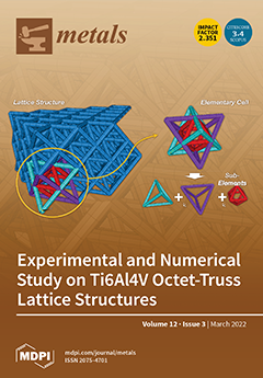
Metal lattice structures produced by means of additive techniques are attracting increasing attention due to their high structural efficiency. However, the current manufacturing processes are still not able to provide defect-free components; therefore, in order to design optimal and reliable configurations, certain aspects must be considered. The present work describes a numerical–experimental procedure to estimate the global loss in stiffness and strength of metal lattice structures due to the manufacturing process used (i.e., EBM). The models were validated with respect to experimental three-point bending tests and by considering two kinds of specimen with octet-truss unit cells and optional outer skins. View this paper
  • Issues are regarded as officially published after their release is announced to the table of contents alert mailing list.
  • You may sign up for e-mail alerts to receive table of contents of newly released issues.
  • PDF is the official format for papers published in both, html and pdf forms. To view the papers in pdf format, click on the "PDF Full-text" link, and use the free Adobe Reader to open them.
Order results
Result details
Section
Select all
Export citation of selected articles as:
16 pages, 7318 KiB  
Article
Evaluation of Microstructural and Mechanical Behavior of AHSS CP780 Steel Welded by GMAW-Pulsed and GMAW-Pulsed-Brazing Processes
by Alan Jadir Romero-Orozco, José Jaime Taha-Tijerina, Rene De Luna-Alanís, Victor Hugo López-Morelos, María del Carmen Ramírez-López, Melchor Salazar-Martínez and Francisco Fernando Curiel-López
Metals 2022, 12(3), 530; https://doi.org/10.3390/met12030530 - 21 Mar 2022
Cited by 5 | Viewed by 2598
Abstract
Joints of complex phase 780 (CP-780) advanced high strength steel (AHSS) were carried out by using an ER-CuAl-A2 filler metal for the gas metal arc welding pulsed brazing (GMAW-P- brazing) process and the ER-80S-D2 for the GMAW-P process employing two levels of heat [...] Read more.
Joints of complex phase 780 (CP-780) advanced high strength steel (AHSS) were carried out by using an ER-CuAl-A2 filler metal for the gas metal arc welding pulsed brazing (GMAW-P- brazing) process and the ER-80S-D2 for the GMAW-P process employing two levels of heat input. The phases in the weld bead and HAZ were analyzed, and the evaporation of zinc by means of scanning electron microscopy (SEM) was also monitored. The mechanical properties of the welded joints were evaluated by tension, microhardness and vertical impact tests. It was found that there was greater surface Zn evaporation in the joints welded with the GMAW-P process as compared to the GMAW-P-brazing process. The best results in tensile strength were observed in the joints welded with GMAW-P-brazing process, which increased by ~68% with respect to those of the GMAW-P. This behavior can be attributed to the formation of an intermetallic complex compound Cu-Al-Fe in the fusion line. Full article
(This article belongs to the Special Issue Mechanical Properties Assessment of Alloys during Welding Process)
Show Figures

Figure 1

Figure 1
<p>(<b>a</b>) Schematic of the lap welded joint and (<b>b</b>) fixture holding the sheets and torch angle.</p>
Full article ">Figure 2
<p>Schematic of the cuts performed in the lap welded joints for characterization.</p>
Full article ">Figure 3
<p>Microstructure of the BM CP 780.</p>
Full article ">Figure 4
<p>SEM observation. (<b>a</b>) microstructure of the BM and (<b>b</b>) EDS analysis.</p>
Full article ">Figure 5
<p>Macrostructural sections of welds. (<b>a</b>) GMAW-P low heat input, (<b>b</b>) GMAW-P high heat input, (<b>c</b>) GMAW-P-brazing low heat input and (<b>d</b>) GMAW-P-brazing high heat input.</p>
Full article ">Figure 6
<p>Microstructural features of the GMA welds: (<b>a</b>) ER80S low heat input, (<b>b</b>) ER80S high heat input, (<b>c</b>) brazing low heat input and (<b>d</b>) brazing high heat input.</p>
Full article ">Figure 7
<p>Line scan in GMA welds: (<b>a</b>) brazing low heat input and (<b>b</b>) brazing high heat input.</p>
Full article ">Figure 8
<p>Microhardness profiles; (<b>a</b>) schematic of the measurements made in the lap welded joints, (<b>b</b>) GMAW-P and (<b>c</b>) GMAW-P-brazing.</p>
Full article ">Figure 9
<p>Failure modes in lap welded joints, adapted from [<a href="#B13-metals-12-00530" class="html-bibr">13</a>].</p>
Full article ">Figure 10
<p>Macrographs of the lap welded joints for pulsed and pulsed-brazing specimens after tensile testing: (<b>a</b>) top view and (<b>b</b>) transverse view.</p>
Full article ">Figure 11
<p>Load versus length curves of the CP lap welded joints.</p>
Full article ">Figure 12
<p>Fracture of the GMA welds with the ER 80S electrode: (<b>a</b>) low heat input, (<b>b</b>) high heat input, (<b>c</b>) analyzed particle and (<b>d</b>) EDS spectrum.</p>
Full article ">Figure 13
<p>Fracture of the GMAW-P-brazing for (<b>a</b>) low heat input and (<b>b</b>) high heat input.</p>
Full article ">Figure 14
<p>Free fall test. (<b>a</b>) GMAW-P low heat input, (<b>b</b>) GMAW-P high heat input, (<b>c</b>) GMAW-P -brazing low heat input and (<b>d</b>) GMAW-P-brazing high heat input.</p>
Full article ">Figure 15
<p>Load versus displacement behavior of the free fall tests, (<b>a</b>) full assay, and (<b>b</b>) amplified zone.</p>
Full article ">
13 pages, 1909 KiB  
Article
Effect of Milling Parameters on Mechanical Properties and In Vitro Biocompatibility of Mg-Zn-Co Ternary Alloy
by Sehrish Mukhtar, Muhammad Kamran, Rafiq Ahmed and Asima Tayyeb
Metals 2022, 12(3), 529; https://doi.org/10.3390/met12030529 - 21 Mar 2022
Cited by 3 | Viewed by 2211
Abstract
Magnesium (Mg) is a potential candidate for biomedical implants, but its susceptibility to suffer corrosion attack in human body fluid limits its practical use. Thus, alloying Mg with other metal elements is the most effective strategy to improve its mechanical properties and biocompatibility. [...] Read more.
Magnesium (Mg) is a potential candidate for biomedical implants, but its susceptibility to suffer corrosion attack in human body fluid limits its practical use. Thus, alloying Mg with other metal elements is the most effective strategy to improve its mechanical properties and biocompatibility. Herein, we report a Mg-Zn-Co ternary alloy (85-10-5 wt %) synthesized by the mechanical alloying technique. Ball-milling parameters such as ball size and milling time were varied to obtain better alloy properties. After compaction and sintering, the obtained alloy samples were subjected to various characterizations, including grain, scanning electron microscopy (SEM), energy-dispersive X-ray spectroscopy, X-ray diffraction (XRD), microhardness and nanoindentation analyses. In vitro biocompatibility analysis of different alloys was also performed with MC3T3-E1 osteoblasts. Grain analysis confirmed the even dispersion of particles, while SEM analysis showed the formation of laminates, spherical and fine particles with an increase in time and varied ball size. XRD results further confirmed the formation of intermetallic compounds. The microhardness of samples was increased with the increase in milling time. The Young’s modulus of ternary alloys obtained from nanoindentation analysis was comparable to the modulus of human bone. Moreover, in vitro analysis with osteoblasts showed that the developed alloys were noncytotoxic and biocompatible. Full article
(This article belongs to the Special Issue Development and Application of Biodegradable Metals)
Show Figures

Figure 1

Figure 1
<p>Morphological analysis of pure constituents of Mg-Zn-Co alloys using SEM: (<b>a</b>) 99.9% pure Mg; (<b>b</b>) 99.9% pure Zn; (<b>c</b>) 99.9% pure Co.</p>
Full article ">Figure 2
<p>Graphical representation of particle size distribution in Mg-Zn-Co alloy samples, prepared via: (<b>a</b>) uniform-sized ball milling (Xhr-U); (<b>b</b>) variable-sized ball milling (Xhr-V).</p>
Full article ">Figure 3
<p>Microstructure analysis of different samples of Mg-Zn-Co alloys using ASTM-E112; (<b>a</b>) 7hr-U; (<b>b</b>) 7hr-V; (<b>c</b>) 15hr-U; (<b>d</b>) 15hr-V; (<b>e</b>) 30hr-U; (<b>f</b>) 30hr-V. Particles shown with different colors represent percentage count with respect to equivalent circumference diameter.</p>
Full article ">Figure 4
<p>Morphological analysis of different samples of Mg-Zn-Co alloys using SEM: (<b>a</b>) 7hr-U; (<b>b</b>) 7hr-V; (<b>c</b>) 15hr-U; (<b>d</b>) 15hr-V; (<b>e</b>) 30hr-U; (<b>f</b>) 30hr-V.</p>
Full article ">Figure 5
<p>Formation of intermetallic compound analysis of Mg-Zn-Co alloys using XRD: (<b>a</b>) 7hr-U; (<b>b</b>) 30hr-U.</p>
Full article ">Figure 6
<p>Microhardness analysis of Mg-Zn-Co alloy using micro-Vickers for both Xhr-U and Xhr-V. (* <span class="html-italic">p</span> &lt; 0.05).</p>
Full article ">Figure 7
<p>In vitro biocompatibility analysis of different mechanically alloyed Mg-Zn-Co alloys. MC3T3-E1 cells were used to analyze biocompatibility test of different combinations. Cells cultured in extract media were analyzed for morphological analysis: (<b>a</b>) control; (<b>b</b>) 7hr-U; (<b>c</b>) 30hr-U. (<b>d</b>) Graphical representation of MTT cell cytotoxicity analysis of cells cultured in different extraction media of alloys compared to control media.</p>
Full article ">
18 pages, 4144 KiB  
Article
Development of Closed-Form Equations for Estimating Mechanical Properties of Weld Metals according to Chemical Composition
by Jeong-Hwan Kim, Chang-Ju Jung, Young IL Park and Yong-Taek Shin
Metals 2022, 12(3), 528; https://doi.org/10.3390/met12030528 - 21 Mar 2022
Cited by 3 | Viewed by 1877
Abstract
In this study, data analysis was performed using an artificial neural network (ANN) approach to investigate the effect of the chemical composition of welds on their mechanical properties (yield strength, tensile strength, and impact toughness). Based on the data collected from previously performed [...] Read more.
In this study, data analysis was performed using an artificial neural network (ANN) approach to investigate the effect of the chemical composition of welds on their mechanical properties (yield strength, tensile strength, and impact toughness). Based on the data collected from previously performed experiments, correlations between related variables and results were analyzed and predictive models were developed. Sufficient datasets were prepared using data augmentation techniques to solve problems caused by insufficient data and to make better predictions. Finally, closed-form equations were developed based on the predictive models to evaluate the mechanical properties according to the chemical composition. Full article
(This article belongs to the Special Issue Modelling, Test and Practice of Steel Structures)
Show Figures

Figure 1

Figure 1
<p>Test assembly for extraction of test pieces: (<b>a</b>) disposition of weld runs; (<b>b</b>) sample extraction overview adapted from [<a href="#B1-metals-12-00528" class="html-bibr">1</a>].</p>
Full article ">Figure 2
<p>(<b>a</b>) CVN impact energy versus temperature and ductile–brittle transition temperature (DBTT); (<b>b</b>) comparison of materials A and B adapted from [<a href="#B17-metals-12-00528" class="html-bibr">17</a>].</p>
Full article ">Figure 3
<p>Example of data augmentation: (<b>a</b>) Mn–0.04C; (<b>b</b>) Mn–0.06C; (<b>c</b>) Mn–0.10C; and (<b>d</b>) Mn–0.15C.</p>
Full article ">Figure 4
<p>Basic structure of the ANN model applied in this study.</p>
Full article ">Figure 5
<p>Sensitivity study for determining the number of hidden layer neurons.</p>
Full article ">Figure 6
<p>Data splitting ratio.</p>
Full article ">Figure 7
<p>Prediction performances: (<b>a</b>) training stage; (<b>b</b>) validation stage; (<b>c</b>) combination of the training and validation stages.</p>
Full article ">Figure 8
<p>Comparison of the estimation and test data in terms of CVN temperature: (<b>a</b>) Mn–0.5Ni; (<b>b</b>) Mn–1.0Ni; (<b>c</b>) Mn–2.25Ni; (<b>d</b>) Mn–3.5Ni.</p>
Full article ">Figure 9
<p>Comparison of the estimation and test data in terms of yield strength: (<b>a</b>) Mn–0.5Ni; (<b>b</b>) Mn–1.0Ni; (<b>c</b>) Mn–2.25Ni; (<b>d</b>) Mn–3.5Ni.</p>
Full article ">Figure 10
<p>Comparison of the estimation and test data in terms of tensile strength: (<b>a</b>) Mn–0.5Ni; (<b>b</b>) Mn–1.0Ni; (<b>c</b>) Mn–2.25Ni; (<b>d</b>) Mn–3.5Ni.</p>
Full article ">Figure A1
<p>Comparison of the estimation and test data in terms of CVN temperature: (<b>a</b>) Mn–0.04C; (<b>b</b>) Mn–0.06C; (<b>c</b>) Mn–0.10C; (<b>d</b>) Mn–0.15C.</p>
Full article ">Figure A2
<p>Comparison of the estimation and test data in terms of CVN temperature: (<b>a</b>) Mn–0.25Cr; (<b>b</b>) Mn–0.5Cr; (<b>c</b>) Mn–1.0Cr; (<b>d</b>) Mn–2.3Cr.</p>
Full article ">Figure A3
<p>Comparison of the estimation and test data in terms of CVN temperature: (<b>a</b>) Mn–0.2Si; (<b>b</b>) Mn–0.4Si; (<b>c</b>) Mn–0.6Si; (<b>d</b>) Mn–0.9Si.</p>
Full article ">Figure A4
<p>Comparison of the estimation and test data in terms of CVN temperature: (<b>a</b>) Mn–0.0Mo; (<b>b</b>) Mn–0.25Mo; (<b>c</b>) Mn–0.5Mo; (<b>d</b>) Mn–1.1Mo.</p>
Full article ">Figure A5
<p>Comparison of the estimation and test data in terms of CVN temperature: (<b>a</b>) Mn–0.03O; (<b>b</b>) Mn–0.037O; (<b>c</b>) Mn–0.045O.</p>
Full article ">Figure A6
<p>Comparison of the estimation and test data in terms of CVN temperature: (<b>a</b>) Mn–0.0004V; (<b>b</b>) Mn–0.02V; (<b>c</b>) Mn–0.04V; (<b>d</b>) Mn–0.06V; (<b>e</b>) Mn–0.08V.</p>
Full article ">Figure A6 Cont.
<p>Comparison of the estimation and test data in terms of CVN temperature: (<b>a</b>) Mn–0.0004V; (<b>b</b>) Mn–0.02V; (<b>c</b>) Mn–0.04V; (<b>d</b>) Mn–0.06V; (<b>e</b>) Mn–0.08V.</p>
Full article ">Figure A7
<p>Comparison of the estimation and test data in terms of CVN temperature: (<b>a</b>) Mn–0.0004Nb; (<b>b</b>) Mn–0.01Nb; (<b>c</b>) Mn–0.02Nb; (<b>d</b>) Mn–0.045Nb; (<b>e</b>) Mn–0.09Nb.</p>
Full article ">
10 pages, 1592 KiB  
Article
The Influence of Thermomechanical Treatments on the Structure, Microstructure, and Mechanical Properties of Ti-5Mn-Mo Alloys
by Mariana Luna Lourenço, Fenelon Martinho Lima Pontes and Carlos Roberto Grandini
Metals 2022, 12(3), 527; https://doi.org/10.3390/met12030527 - 21 Mar 2022
Cited by 5 | Viewed by 2017
Abstract
With the increase in the world’s population, the rising number of traffic accidents, and the increase in life expectancy, the need for implants, dental work, and orthopedics is growing ever larger. Researchers are working to improve the biomaterials used for these purposes, improve [...] Read more.
With the increase in the world’s population, the rising number of traffic accidents, and the increase in life expectancy, the need for implants, dental work, and orthopedics is growing ever larger. Researchers are working to improve the biomaterials used for these purposes, improve their functionality, and increase the human body’s life span. Thus, new titanium alloys are being developed, usually with β-stabilizer elements (which decrease the elastic modulus), with the Ti-Mn-Mo alloys being one example of these. This study of the Ti-5Mn-10Mo and Ti-5Mn-15Mo alloys only showed signs of the β phase in the structure and microstructure, presenting a combination of low modulus of elasticity and high corrosion resistance compared to the values of commercial alloys. In this sense, this work presents an analysis of the influence of some thermomechanical treatments, such as homogenization, hot-rolling, solution, and annealing, on the structure, microstructure, and selected mechanical properties of the Ti-5Mn-10Mo and Ti-5Mn-15Mo alloys. Full article
(This article belongs to the Special Issue Innovations in Metallic Biomaterials)
Show Figures

Figure 1

Figure 1
<p>X-ray diffractograms for Ti-5Mn-10Mo alloy after homogenization heat treatment (<b>a</b>), after the hot-rolling process (<b>b</b>), and after the solution (<b>c</b>) and annealing (<b>d</b>) heat treatments.</p>
Full article ">Figure 2
<p>X-ray diffractograms for Ti-5Mn-15Mo alloy after homogenization heat treatment (<b>a</b>), after the hot-rolling process (<b>b</b>), and after the solution (<b>c</b>) and annealing (<b>d</b>) heat treatments.</p>
Full article ">Figure 3
<p>Optical micrographs of the Ti-5Mn-10Mo alloy after homogenization (<b>a</b>), hot-rolling (<b>b</b>), and solution (<b>c</b>) and annealing (<b>d</b>) treatments. SEM micrographs of the Ti-5Mn-10Mo alloy after homogenization (<b>e</b>), hot-rolling (<b>f</b>), and solution (<b>g</b>) and annealing (<b>h</b>) treatments.</p>
Full article ">Figure 4
<p>Optical micrographs of the Ti-5Mn-15Mo alloy after homogenization (<b>a</b>), hot-rolling (<b>b</b>), and solution (<b>c</b>) and annealing (<b>d</b>) treatments. SEM micrographs of the Ti-5Mn-15Mo alloy after homogenization (<b>e</b>), hot-rolling (<b>f</b>), and solution (<b>g</b>) and annealing (<b>h</b>) treatments.</p>
Full article ">Figure 5
<p>Microhardness for Ti-5Mn-10Mo and Ti-5Mn-15Mo alloys under all processing conditions compared to CP-Ti.</p>
Full article ">Figure 6
<p>Comparison of Young’s modulus of the Ti-5Mn-10Mo and Ti-5Mn-15Mo alloys with commercial alloys under all processing conditions.</p>
Full article ">
15 pages, 5372 KiB  
Article
Research on High-Temperature Compressive Properties of Ti–10V–1Fe–3Al Alloy
by Cong Li, Can Huang, Zhili Ding and Xing Zhou
Metals 2022, 12(3), 526; https://doi.org/10.3390/met12030526 - 21 Mar 2022
Cited by 2 | Viewed by 1763
Abstract
To investigate the thermal deformation behavior of Ti–10V–2Cr–3Al titanium alloy, the hot compression experiments were carried out via a strain rate of 0.1–0.001 s−1 and deformation temperature of 730~880 °C. The results showed that the rheological stress decreases when the deformation temperature [...] Read more.
To investigate the thermal deformation behavior of Ti–10V–2Cr–3Al titanium alloy, the hot compression experiments were carried out via a strain rate of 0.1–0.001 s−1 and deformation temperature of 730~880 °C. The results showed that the rheological stress decreases when the deformation temperature increases or strain rate decreases. Due to the deformation conditions, some flow curves exhibited significant discontinuous yielding and flow softening. Flow softening in the α+β phase region was dominated by dynamic recrystallization (DRX), while in the β phase region, it was centered on dynamic recovery (DRV). A high-temperature constitutive equation, with good predictive power, was established. Full article
Show Figures

Figure 1

Figure 1
<p>The initial microstructure of Ti–10V–1Fe–3Al alloy.</p>
Full article ">Figure 2
<p>True stress-true strain curve: (<b>a</b>) 730, (<b>b</b>) 790, (<b>c</b>) 820, and (<b>d</b>) 880 °C.</p>
Full article ">Figure 3
<p>(<b>a</b>) Linear fitting of <span class="html-italic">σ</span>–<span class="html-italic">lnέ</span>; (<b>b</b>) linear fitting of <span class="html-italic">lnσ</span>–<span class="html-italic">lnέ</span>.</p>
Full article ">Figure 4
<p>(<b>a</b>) The relationship between the flow stress (<span class="html-italic">σ</span>) and deformation temperature (<span class="html-italic">T</span><sup>−1</sup>). (<b>b</b>) Fitting relationship between the experimental flow stress and predicted flow stress, when the strain is 0.1.</p>
Full article ">Figure 5
<p>The relationship between the constants and strain: (<b>a</b>) the material constant (<span class="html-italic">b</span>), (<b>b</b>) deformation activation energy <span class="html-italic">Q</span> value, and (<b>c</b>) material constant (<span class="html-italic">lnA</span>).</p>
Full article ">Figure 6
<p>Fitting curve of n value.</p>
Full article ">Figure 7
<p>The relationship between <span class="html-italic">ln</span>(<span class="html-italic">sinh</span>(<span class="html-italic">ασ</span>)) and the deformation temperature (<span class="html-italic">T</span><sup>−1</sup>).</p>
Full article ">Figure 8
<p>The relationship between various constants and strain: (<b>a</b>) <span class="html-italic">ε-α</span> diagram, (<b>b</b>) <span class="html-italic">ε</span>-1/<span class="html-italic">n</span> diagram, (<b>c</b>) <span class="html-italic">ε-Q</span> diagram, (<b>d</b>) <span class="html-italic">ε-</span><span class="html-italic">lnA</span> diagram, and (<b>e</b>) <span class="html-italic">ε-m</span> diagram.</p>
Full article ">Figure 9
<p>Contrast between experimental flow stress (solid line) and predicted flow stress (dot line): (<b>a</b>) 730, (<b>b</b>) 790, (<b>c</b>) 820, and (<b>d</b>) 880 °C.</p>
Full article ">Figure 9 Cont.
<p>Contrast between experimental flow stress (solid line) and predicted flow stress (dot line): (<b>a</b>) 730, (<b>b</b>) 790, (<b>c</b>) 820, and (<b>d</b>) 880 °C.</p>
Full article ">Figure 10
<p>Fitting relationship between experimental and predicted flow stress.</p>
Full article ">Figure 11
<p>High-temperature compression microstructure of Ti–10V–1Fe–3Al alloy at strain rate of 0.01 s<sup>−1</sup>: (<b>a</b>) 730, (<b>b</b>) 790, (<b>c</b>) 820, and (<b>d</b>) 880 °C.</p>
Full article ">
10 pages, 5102 KiB  
Article
Structure and Properties of Metal-Matrix Composites Based on an Inconel 625–TiB2 System Fabricated by Additive Manufacturing
by Vladimir Promakhov, Alexey Matveev, Olga Klimova-Korsmik, Nikita Schulz, Vladislav Bakhmat, Artem Babaev and Alexander Vorozhtsov
Metals 2022, 12(3), 525; https://doi.org/10.3390/met12030525 - 21 Mar 2022
Cited by 8 | Viewed by 2708
Abstract
This research work studies the structural phase parameters and physicomechanical properties of metal-matrix composite materials based on a Ni–TiB2 system obtained by additive manufacturing (specifically, direct laser deposition). The properties of the composites obtained were investigated at high temperatures (up to 1000 [...] Read more.
This research work studies the structural phase parameters and physicomechanical properties of metal-matrix composite materials based on a Ni–TiB2 system obtained by additive manufacturing (specifically, direct laser deposition). The properties of the composites obtained were investigated at high temperatures (up to 1000 °C). The feasibility of the fabrication of a composite nanostructure of alloy with advanced physicomechanical properties was shown. The introduction of reinforcing TiB2 particles into an Inconel 625 matrix was confirmed to increase the microhardness and tensile strength of the material obtained. Apparently, the composite structure of the samples facilitates the realisation of several strengthening mechanisms: (1) a grain boundary mechanism that causes strengthening and dislocation movement; (2) a mechanism based on the grain structure breakdown and Hall–Petch relationship realisation. Full article
Show Figures

Figure 1

Figure 1
<p>SEM image of Inconel 625 powder particles and histogram of their distribution by size (<b>a</b>,<b>b</b>); SEM image of the structure of NiTi–TiB<sub>2</sub> composite powder particles and histogram of TiB<sub>2</sub> particle size distribution in the NiTi matrix (<b>c</b>,<b>d</b>).</p>
Full article ">Figure 2
<p>Ytterbium fibre laser LS-3 (<b>a</b>); concurrent dual-side deposition strategy (<b>b</b>).</p>
Full article ">Figure 3
<p><b>(a)</b> Appearance of the materials obtained by selective laser deposition from a powder mixture consisting of 95 wt% Inconel 625 + 5 wt% NiTi–TiB<sub>2</sub>; (<b>b</b>) X-ray pattern of the obtained materials; (<b>c</b>,<b>d</b>) SEM images of the structure of the materials; (<b>e</b>) size distribution of TiB<sub>2</sub> particles in these materials.</p>
Full article ">Figure 4
<p><b>(a)</b> Appearance of the materials obtained by direct laser deposition from a powder mixture of 95 wt% Inconel 625 + 5 wt% NiTi–TiB<sub>2</sub>; (<b>b</b>) a schematic of the distribution of indenter marks on the sample; (<b>c</b>) a diagram of the distribution of hardness values in the sample.</p>
Full article ">Figure 5
<p>(<b>a</b>) Diagram of specimens for stress testing; (<b>b</b>) stress–strain diagram obtained during tensile testing of samples obtained by the deposition of a powder mixture of 95 wt% Inconel 625 + 5 wt% NiTi–TiB<sub>2</sub> powder mixture, as well as from testing the samples deposited from pure Inconel 625.</p>
Full article ">Figure 6
<p>(<b>a</b>) Appearance of the three-point bending tester; (<b>b</b>) a schematic representation of the shape and dimensions of the 95 wt% Inconel 625 + 5 wt% NiTi–TiB<sub>2</sub> sample; dependencies of bending strength and bending deformation rate of samples after three-point bending tests conducted at room (<b>c</b>) and at elevated (<b>d</b>) temperatures.</p>
Full article ">
15 pages, 6088 KiB  
Article
Preparation of Ti-46Al-8Nb Alloy Ingots beyond Laboratory Scale Based on BaZrO3 Refractory Crucible
by Baohua Duan, Lu Mao, Yuchen Yang, Qisheng Feng, Xuexian Zhang, Haitao Li, Lina Jiao, Rulin Zhang, Xionggang Lu, Guangyao Chen and Chonghe Li
Metals 2022, 12(3), 524; https://doi.org/10.3390/met12030524 - 21 Mar 2022
Cited by 4 | Viewed by 2731
Abstract
The high Nb-containing TiAl-based alloy ingot beyond laboratory scale with a composition of Ti-46Al-8Nb (at.%) was prepared by a vacuum induction melting process based on a BaZrO3 refractory crucible. A round bar ingot with a diameter of 85 mm and a length [...] Read more.
The high Nb-containing TiAl-based alloy ingot beyond laboratory scale with a composition of Ti-46Al-8Nb (at.%) was prepared by a vacuum induction melting process based on a BaZrO3 refractory crucible. A round bar ingot with a diameter of 85 mm and a length of 430 mm was finally obtained, and the chemical composition, solidification pathway, microstructure and tensile properties of the ingot were investigated. The results show that the deviations of Al and Nb content along a 430 mm long central part of the ingot are approximately ±0.39 at.% and ±0.14 at.%, and the oxygen content in the ingot can be controlled at around 1000 ppm. The structure of the alloy ingot is a full lamellar structure composed of γ and α2 phases, and the thickness of the lamellae is approximately 0.53 μm. In case of the α2 phase, the surface content of the ingot is higher than the middle region and the centrical region; also, it indicated a decreasing trend. During cooling, the alloy solidified from a peritectic reaction (L + β→α) rather than the solidified via β phase (β→α). In addition to Al segregation and Nb segregation, β-phase particles associated with γ phase at the triple junction of the colonies were observed. Moreover, the tensile properties of the longitudinal-cut sample in the ingot is significantly better than those of the transverse-cut sample, with a tensile strength of up to as high as 700 MPa and a corresponding fracture elongation of 1.1%. However, the tensile strength of the transverse-cut sample is only 375 MPa, and the fracture elongation is 0.52%. Full article
(This article belongs to the Special Issue Light Alloy and Its Application)
Show Figures

Figure 1

Figure 1
<p>Schematic diagram of the Ti-46Al-8Nb alloy melting process. (<b>a</b>) Schematic of a vacuum induction melting furnace; (<b>b</b>) BaZrO<sub>3</sub> refractory crucible; (<b>c</b>) Obtained Ti-46Al-8Nb alloy ingot.</p>
Full article ">Figure 2
<p>The melting power and corresponding holding time.</p>
Full article ">Figure 3
<p>Schematic diagram of sampling. (<b>a</b>) Schematic of the Ti-46Al-8Nb alloy ingot; (<b>b</b>) 2 mm thick transverse slice and ingot cut in half longitudinally; (<b>c</b>) Tensile specimen and its corresponding sizes.</p>
Full article ">Figure 4
<p>Pseudo-binary phase diagram of Ti-Al with 8 at.% Nb concentration [<a href="#B44-metals-12-00524" class="html-bibr">44</a>].</p>
Full article ">Figure 5
<p>X-ray diffraction spectra of the ingot obtained at different location. The locations of samples A, B and C are shown in <a href="#metals-12-00524-f003" class="html-fig">Figure 3</a>.</p>
Full article ">Figure 6
<p>Structure of the transverse section of the alloy ingot. (<b>a</b>) Macrograph from surface to core; (<b>b</b>–<b>d</b>) are the metallographic structures of sample A, sample B and sample C, respectively.</p>
Full article ">Figure 7
<p>The microstructure characterization and line scan analysis of the transverse section were carried out under SEM-EDS. (<b>a</b>,<b>b</b>) are the microtopography and line scan analysis of the transverse section (Sample B), respectively; (<b>c</b>) is a magnified view of the area in the yellow solid frame in (<b>a</b>).</p>
Full article ">Figure 8
<p>Structure of the longitudinal section of the alloy ingot. (<b>a</b>) Macrograph of longitudinal section, and the sampling location is shown in <a href="#metals-12-00524-f003" class="html-fig">Figure 3</a>; (<b>b</b>–<b>d</b>) are the SEM diagram of longitudinal section.</p>
Full article ">Figure 9
<p>Tensile properties and fracture morphologies of longitudinal and transverse sections. (<b>a</b>) Structural diagram of longitudinal section of the VIM-BZO alloy ingot; (<b>b</b>) stress-strain curve, LS: longitudinal section; TS: transverse section; (<b>c</b>,<b>d</b>) are the fracture morphologies of the transverse-cut tensile sample and the longitudinal-cut tensile sample, respectively.</p>
Full article ">
11 pages, 7333 KiB  
Article
Three-Dimensional Morphology and Analysis of Widmanstätten Sideplates Ferrite
by Shengli Cao, Shaowen Wu, Caijun Zhang and Qingjun Zhang
Metals 2022, 12(3), 523; https://doi.org/10.3390/met12030523 - 21 Mar 2022
Viewed by 2416
Abstract
The three-dimensional (3D) morphology and crystal structure of Widmanstätten sideplate ferrite were simulated using a focused ion beam (FIB) scanning electron microscope equipped with electron backscatter diffraction (EBSD). The primary Widmanstätten sideplates nucleated and grew directly at the austenite grain boundary (GB). A [...] Read more.
The three-dimensional (3D) morphology and crystal structure of Widmanstätten sideplate ferrite were simulated using a focused ion beam (FIB) scanning electron microscope equipped with electron backscatter diffraction (EBSD). The primary Widmanstätten sideplates nucleated and grew directly at the austenite grain boundary (GB). A certain included angle between the sideplates and the austenite GB was observed. The sideplates grew approximately parallel to the grain, and were separated by a small-angle GB. The primary Widmanstätten sideplates are best described as “∃” shaped, with a long intermediate ferrite strip. The interface with the austenite GB was smooth and flat, and the sideplate surface contained pits and holes. The secondary Widmanstätten sideplates nucleated and grew on the surface of the proeutectoid GB ferrite, with the sideplates and GB ferrite perpendicular to each other. Sideplates parallel to one another grew into the grain, and were separated by small-angle GB. The 3D morphology was distinguished by its “comb” shape. The sideplates’ tail was clustered and its front end remained sharp. The contact side of the GB ferrite was smooth and flat. The surface contained several uneven pits and defects. Full article
Show Figures

Figure 1

Figure 1
<p>Classification of Widmanstätten ferrite. (<b>a</b>) Primary Widmanstätten sideplates, (<b>b</b>) Secondary Widmanstätten sideplates, (<b>c</b>) Primary Widmanstätten sawteeth, (<b>d</b>) Secondary Widmanstätten sawteeth.</p>
Full article ">Figure 2
<p>Schematic diagram of cutting sample.</p>
Full article ">Figure 3
<p>Scanning electron microscopy (SEM) image of primary Widmanstätten sideplates cutting process. (<b>a</b>) 110th layer, (<b>b</b>) 114th layer, (<b>c</b>) 117th layer, (<b>d</b>) 119th layer, (<b>e</b>) 127th layer, (<b>f</b>) 131st layer.</p>
Full article ">Figure 4
<p>Grain orientation of primary Widmanstätten sideplates cutting process. (<b>a</b>) 110th layer, (<b>b</b>) 114th layer, (<b>c</b>) 117th layer, (<b>d</b>) 119th layer, (<b>e</b>) 127th layer, (<b>f</b>) 131st layer.</p>
Full article ">Figure 4 Cont.
<p>Grain orientation of primary Widmanstätten sideplates cutting process. (<b>a</b>) 110th layer, (<b>b</b>) 114th layer, (<b>c</b>) 117th layer, (<b>d</b>) 119th layer, (<b>e</b>) 127th layer, (<b>f</b>) 131st layer.</p>
Full article ">Figure 5
<p>GB orientation of primary Widmanstätten sideplates cutting process. (<b>a</b>) 119th layer, (<b>b</b>) 127th layer.</p>
Full article ">Figure 6
<p>3D morphology of primary Widmanstätten sideplates from different perspectives. (<b>a</b>) X–Y, (<b>b</b>) X–Z, (<b>c</b>) Y–Z.</p>
Full article ">Figure 7
<p>Primary Widmanstätten sideplate growth. (<b>a</b>) Nucleation, (<b>b</b>) growth.</p>
Full article ">Figure 8
<p>2D SEM image of the secondary Widmanstätten sideplate cutting process. (<b>a</b>) 51st layer, (<b>b</b>) 59th layer, (<b>c</b>) 62nd layer, (<b>d</b>) 68th layer, (<b>e</b>) 72nd layer, (<b>f</b>) 93rd layer.</p>
Full article ">Figure 9
<p>Grain orientation of secondary Widmanstätten cutting process. (<b>a</b>) 51st layer, (<b>b</b>) 59th layer, (<b>c</b>) 62nd layer, (<b>d</b>) 68th layer, (<b>e</b>) 72nd layer, (<b>f</b>) 93rd layer.</p>
Full article ">Figure 10
<p>Accumulated misorientation of red line in <a href="#metals-12-00523-f009" class="html-fig">Figure 9</a>e.</p>
Full article ">Figure 11
<p>GB orientation of secondary Widmanstätten sideplates cutting process. (<b>a</b>) 62nd layer, (<b>b</b>) 72nd layer.</p>
Full article ">Figure 12
<p>3D morphology of secondary Widmanstätten sideplates from different perspectives. (<b>a</b>) X–Y, (<b>b</b>) X–Z, (<b>c</b>) Y–Z.</p>
Full article ">Figure 13
<p>Diagram of secondary Widmanstätten sideplates growth. (<b>a</b>) GB ferrite nucleates at GBs, (<b>b</b>) Larger GB ferrite is formed, (<b>c</b>) Secondary Widmanstätten sideplates nucleate at grain boundary ferrite, (<b>d</b>) Secondary Widmanstätten sideplates growth.</p>
Full article ">
13 pages, 3210 KiB  
Article
Experimental and Modeling Study of Deformability of Glassy CaO-(MnO)-Al2O3-SiO2 Inclusions
by Qifeng Shu, Chaoge You, Tuomas Alatarvas and Timo Matti Juhani Fabritius
Metals 2022, 12(3), 522; https://doi.org/10.3390/met12030522 - 20 Mar 2022
Cited by 4 | Viewed by 2342
Abstract
The occurrence of non-deformable, non-metallic inclusions is the dominant reason for failure of wire during drawing and degrades service life for some steel grades, e.g., tire cord steel. To investigate the deformability of glassy inclusions in CaO-Al2O3-SiO2 and [...] Read more.
The occurrence of non-deformable, non-metallic inclusions is the dominant reason for failure of wire during drawing and degrades service life for some steel grades, e.g., tire cord steel. To investigate the deformability of glassy inclusions in CaO-Al2O3-SiO2 and MnO-Al2O3-SiO2 systems, experimental and numerical methods were used. Young’s modulus values of some glasses based on the CaO-Al2O3-SiO2 and MnO-Al2O3-SiO2 systems, which correspond to typical inclusions in tire cord steel, were measured with resonant ultrasound spectroscopy. The effect of basicity, defined as the ratio of mass percentage of CaO to SiO2, on Young’s modulus and Poisson’s ratio were investigated. The Young’s moduli of glasses are enhanced with increasing basicity, which could be attributed to the high field strength of calcium ions. The Poisson’s ratios of glasses also show an increase tendency with increasing basicity, which could be due to the loss of rigidity of network with introduction of calcium ions. The equations in the literature for Young’s modulus calculation were evaluated based on the present and literature data. Appen’s equation is modified by re-fitting the present and literature data to give accurate estimation of Young’s modulus with the mean deviation of 2%. The iso-Young’s modulus diagrams for CaO-Al2O3-SiO2 systems were constructed. It is proposed that the iso-Young’s modulus diagram could be combined with liquid area in CaO-Al2O3-SiO2 ternary phase diagram to optimize the inclusion composition during both hot rolling and cold drawing. Full article
(This article belongs to the Special Issue Inclusion Precipitation during Solidification of Steels)
Show Figures

Figure 1

Figure 1
<p>The XRD pattern for samples showing the glassy state of samples.</p>
Full article ">Figure 2
<p>The measured Young’s modulus values as a function of basicity (w(CaO)/w(SiO<sub>2</sub>)).</p>
Full article ">Figure 3
<p>The measured Poisson’s ratios values as a function of basicity (w(CaO)/w(SiO<sub>2</sub>)).</p>
Full article ">Figure 4
<p>Comparison between measured and calculated Young’s modulus data.</p>
Full article ">Figure 5
<p>Iso-Young’s modulus diagrams of CaO-Al<sub>2</sub>O<sub>3</sub>-SiO<sub>2</sub> system constructed by various equations. (<b>a</b>) Winkmann–Schott. (<b>b</b>) Appen. (<b>c</b>) Ashizuka–Zhang. (<b>d</b>) Modified Appen.</p>
Full article ">Figure 6
<p>The liquid area at 1673–1773 K and iso-Young’s modulus (in GPa) diagram calculated from modified Appen’s equation for CaO-Al<sub>2</sub>O<sub>3</sub>-SiO<sub>2</sub> system.</p>
Full article ">
17 pages, 6935 KiB  
Article
Effect of Corrugated Sheet Diameter on Structural Behavior under Cryogenic Temperature and Hydrodynamic Load
by Jin-Seok Park, Jeong-Hyeon Kim, Yong-Cheol Jeong, Hee-Tae Kim, Seul-Kee Kim and Jae-Myung Lee
Metals 2022, 12(3), 521; https://doi.org/10.3390/met12030521 - 18 Mar 2022
Cited by 1 | Viewed by 2426
Abstract
The most important technical issue in the shipbuilding industry regarding liquefied natural gas (LNG) carrier cargo containment systems (CCS) is securing the structural reliability of the primary barrier, which is in direct contact with the LNG. Fracture of the primary barrier by the [...] Read more.
The most important technical issue in the shipbuilding industry regarding liquefied natural gas (LNG) carrier cargo containment systems (CCS) is securing the structural reliability of the primary barrier, which is in direct contact with the LNG. Fracture of the primary barrier by the hydrodynamic load of the LNG CCS may lead to disasters because it is difficult to implement immediate safety measures in the marine environment, unlike on land. Hence, structural reliability of the LNG membrane is the most critical issue in LNG carrier CCSs, where thin and corrugated 304L stainless steel is often used as the primary barrier to prevent repeated thermal deformation from the temperature difference during loading (−163 °C) and unloading (20 °C) of the LNG. However, plastic deformation of the 1.2 mm-thick corrugated membrane of the LNG CCS has been reported continuously owing to its vulnerability to cryogenic hydrodynamic loads. In the present study, we conducted a parametric analysis to investigate the effects of the corrugation shape as a preliminary study of the primary barrier. Finite element analysis was conducted with a simplified plate to focus on the effects of corrugation. Furthermore, a two-step validation was conducted using the above experimental results to ensure reliability of the structural analysis. The results show that optimizing the corrugation shape could ensure better structural safety than the conventional design. Full article
(This article belongs to the Special Issue Low-Temperature Behavior of Metals)
Show Figures

Figure 1

Figure 1
<p>(<b>a</b>) Photograph of the primary barrier. (<b>b</b>) Simplified primary barrier without knot area for FEA. (<b>c</b>) Schematic of hydrodynamic loading caused by ship motion. The black arrow represents the flow direction. (<b>d</b>) Schematic of the membrane-type LNG CCS [<a href="#B9-metals-12-00521" class="html-bibr">9</a>].</p>
Full article ">Figure 2
<p>(<b>a</b>) Detailed SPB drawing: (<b>b</b>) front view of SPB, (<b>c</b>) half-length model, and (<b>d</b>) quarter model.</p>
Full article ">Figure 3
<p>(<b>a</b>) Stress–strain curve of AISI 304L tensile test at −163 °C; (<b>b</b>) thermal expansion coefficient of AISI 304L at room and cryogenic temperature.</p>
Full article ">Figure 4
<p>Loading and boundary conditions in (<b>a</b>) symmetric hydrodynamic pressure, (<b>b</b>) thermal shrinkage, and (<b>c</b>) asymmetric hydrodynamic pressure analysis. The red rectangles represent the flat bottom of the SPB, and each line represents a side of the SPB. Furthermore, the gray arrows indicating the pressure direction do not cross the yellow pressure limit line.</p>
Full article ">Figure 5
<p>Schematic of mesh size distribution in (<b>a</b>) symmetric and asymmetric hydrodynamic pressure analysis and (<b>b</b>) thermal shrinkage analysis.</p>
Full article ">Figure 6
<p>Maximum deformation according to the number of elements in (<b>a</b>) pressure tests and (<b>b</b>) thermal shrinkage analysis. The red dashed line connotes deformation convergence.</p>
Full article ">Figure 7
<p>Photographs of the (<b>a</b>) experimental apparatus and (<b>b</b>) strain measurement points at the primary barrier; graphs depicting the (<b>c</b>) tensile properties of AISI 304L at room temperature and (<b>d</b>) experimental and FEA time–strain histories [<a href="#B9-metals-12-00521" class="html-bibr">9</a>].</p>
Full article ">Figure 8
<p>Stress distribution for case No. 32 in (<b>a</b>) symmetric pressure analysis, (<b>b</b>) thermal shrinkage analysis, and (<b>c</b>) asymmetric pressure analysis. The black dashed rectangle and purple dot represent the points under maximum stress. Side view 1 (pressure) represents the pressure side, and side view 2 (nonpressure) represents the opposite case.</p>
Full article ">Figure 9
<p>Deformed shapes for case No. 32 in (<b>a</b>) symmetric pressure analysis, (<b>b</b>) thermal shrinkage analysis, and (<b>c</b>) asymmetric pressure analysis. The black dashed rectangle represents the area of maximum deformation; side view 1 (pressure) shows the face exposed to pressure, and side view 2 (nonpressure) represents the opposite case.</p>
Full article ">Figure 10
<p>Deformation direction of the SPB on the length–middle section in the (<b>a</b>) symmetric pressure analysis, (<b>b</b>) asymmetric pressure analysis, and (<b>c</b>) thermal shrinkage analysis. The black arrows represent the deformation direction of the node from the red line to the blue dashed line.</p>
Full article ">Figure 11
<p>Deformed SPB shapes of 82.8° fillet angle under asymmetric pressure in (<b>a</b>) case No. 12, (<b>b</b>) case No. 22, (<b>c</b>) case No. 32, and (<b>d</b>) case No. 42.</p>
Full article ">Figure 12
<p>Maximum SPB stress and deformation according to the fillet angle in each test (<b>a</b>,<b>c</b>) symmetric pressure analysis and (<b>b</b>,<b>d</b>) asymmetric pressure analysis.</p>
Full article ">Figure 12 Cont.
<p>Maximum SPB stress and deformation according to the fillet angle in each test (<b>a</b>,<b>c</b>) symmetric pressure analysis and (<b>b</b>,<b>d</b>) asymmetric pressure analysis.</p>
Full article ">Figure 13
<p>Maximum (<b>a</b>) stress, stress on the center corrugation, and (<b>b</b>) deformation of SPB according to the fillet angle in thermal shrinkage analysis. The dashed line represents the enlarged region of the graphs.</p>
Full article ">
10 pages, 6111 KiB  
Article
Effects of Extrusion and Rolling Processes on the Microstructure and Mechanical Properties of Zn-Li-Ag Alloys
by Yujiao Lu, Ying Liu, Yilong Dai, Yang Yan and Kun Yu
Metals 2022, 12(3), 520; https://doi.org/10.3390/met12030520 - 18 Mar 2022
Cited by 2 | Viewed by 2832
Abstract
In this work, a novel Zn-0.5%Li-0.1%Ag alloy was cast and extruded into rods, which were rolled into a plate, and the effects of extrusion and rolling on the microstructure and mechanical properties of the Zn-0.5%Li-0.1%Ag alloy were evaluated. The results show that grain [...] Read more.
In this work, a novel Zn-0.5%Li-0.1%Ag alloy was cast and extruded into rods, which were rolled into a plate, and the effects of extrusion and rolling on the microstructure and mechanical properties of the Zn-0.5%Li-0.1%Ag alloy were evaluated. The results show that grain strengthening occurs in all of the alloys because of the presence of nano-LiZn4 precipitates. The extrusion and rolling processes promote grain size refinement and orientation order, and the microstructure and mechanical properties of the Zn-0.5%Li-0.1%Ag alloy can be significantly improved by secondary processing. The elastic modulus and tensile strength of the processed alloy increased to 83.1 GPa and 251.6 MPa, respectively, compared to 75.6 GPa and 185.8 MPa, respectively, for the as-cast Zn-0.5%Li-0.1%Ag alloy. More importantly, elongation was greatly improved, from 16.9% to 92.6%, which is an increase of up to 448%, and there were transgranular cleavage planes and intergranular cleavage planes in the fracture surfaces. The intergranular cleavage planes were dominant, and they showed ductile fracture characteristics. Full article
Show Figures

Figure 1

Figure 1
<p>Schematic diagram of the fabrication process of the Zn-0.5%Li-0.1%Ag alloy.</p>
Full article ">Figure 2
<p>Optical images of the microstructure of the Zn-0.5%Li-0.1%Ag alloy in different treatment states: (<b>a</b>) as-cast, (<b>b</b>) extruded, and (<b>c</b>) rolled.</p>
Full article ">Figure 3
<p>SEM microstructures and EDS analyses of the Zn-0.5%Li-0.1%Ag alloy in different treatment states: (<b>a</b>,<b>b</b>) as-cast, (<b>c</b>,<b>d</b>) extruded, and (<b>e</b>,<b>f</b>) rolled.</p>
Full article ">Figure 4
<p>XRD analyses of the Zn-0.5%Li-0.1%Ag alloy in different treatment states.</p>
Full article ">Figure 5
<p>TEM images of the Zn-0.5%Li-0.1%Ag alloy: (<b>a</b>) low magnification microstructure and (<b>b</b>) high magnification microstructure.</p>
Full article ">Figure 6
<p>Mechanical properties of the Zn-0.5%Li-0.1%Ag alloy in different treatment states.</p>
Full article ">Figure 7
<p>Tensile fracture morphologies of the Zn-0.5%Li-0.1%Ag alloy in different treatment states: (<b>a</b>) as-cast, (<b>b</b>) extruded, and (<b>c</b>) rolled.</p>
Full article ">
11 pages, 3614 KiB  
Article
The Effect of Wall Thickness and Scanning Speed on the Martensitic Transformation and Tensile Properties of Selective Laser Melted NiTi Thin-Wall Structures
by Fangmin Guo, Yanbao Guo, Xiangguang Kong, Zhiwei Xiong and Shijie Hao
Metals 2022, 12(3), 519; https://doi.org/10.3390/met12030519 - 18 Mar 2022
Cited by 4 | Viewed by 2180
Abstract
In this study, we analyzed the coupling effect of laser scanning speed and wall thickness on the phase transformation behavior and tensile properties of selective laser melted NiTi thin-wall structures. It is demonstrated that either scanning speed or wall thickness has their respective [...] Read more.
In this study, we analyzed the coupling effect of laser scanning speed and wall thickness on the phase transformation behavior and tensile properties of selective laser melted NiTi thin-wall structures. It is demonstrated that either scanning speed or wall thickness has their respective influence rule, whereas this influence could be changed when coupling them together; that is, under different scanning speeds, the effect of wall thickness could be different. It is found that the deviation of phase transformation temperature among different wall thicknesses is ~3.7 °C at 400 mm/s, while this deviation increases to ~23.5 °C at 600 mm/s. However, the deviation of phase transformation peak width among different wall thicknesses shows little change under different scanning speeds. At low scanning speed, the samples with thicker wall thickness exhibit better tensile ductility than thinner, whereas they all show poor tensile properties and brittle behavior at high scanning speed. This uncertain influence rule is mainly due to the interaction effect between different thermal histories generated by wall thickness and scanning speed. Full article
(This article belongs to the Special Issue Shape Memory Alloys 2022)
Show Figures

Figure 1

Figure 1
<p>(<b>a</b>) Illustration of the orthogonal-type laser scanning strategy; (<b>b</b>) the NiTi plate samples were fabricated by SLM.</p>
Full article ">Figure 2
<p>Optical micrographs of SLM-NiTi thin-wall structures fabricated by different laser scanning speeds: (<b>a</b>) 400 mm/s, (<b>b</b>) 600 mm/s, (<b>c</b>) 800 mm/s, and (<b>d</b>) 1000 mm/s.</p>
Full article ">Figure 3
<p>The evolutions of porosity with (<b>a</b>) scanning speed and (<b>b</b>) wall thickness.</p>
Full article ">Figure 4
<p>Optical micrographs of thin-wall structures along the build direction with different thickness under scanning speed of 800 mm/s: (<b>a</b>) 0.4 mm, (<b>b</b>) 0.6 mm, (<b>c</b>) 0.8 mm, (<b>d</b>) 1.2 mm, (<b>e</b>) 2.0 mm, and (<b>f</b>) 4.0 mm.</p>
Full article ">Figure 5
<p>The DSC curves of SLM-NiTi thin-wall structures fabricated with different laser scanning speeds: (<b>a</b>) 400 mm/s, (<b>b</b>) 600 mm/s, (<b>c</b>) 800 mm/s, and (<b>d</b>) 1000 mm/s.</p>
Full article ">Figure 6
<p>The martensitic transformation starting temperature (<span class="html-italic">M<sub>s</sub></span>) and martensitic transformation peak width (Δ<span class="html-italic">M</span> = <span class="html-italic">M<sub>s</sub></span> − <span class="html-italic">M<sub>f</sub></span>) of SLM-NiTi thin-wall structures as a function of wall thickness and laser scanning speed: (<b>a</b>) evolution of <span class="html-italic">M<sub>s</sub></span> with scanning speed; (<b>b</b>) evolution of Δ<span class="html-italic">M</span> with scanning speed; (<b>c</b>) evolution of <span class="html-italic">M<sub>s</sub></span> with wall thickness; (<b>d</b>) evolution of Δ<span class="html-italic">M</span> with wall thickness.</p>
Full article ">Figure 7
<p>The stress–strain curves of the samples fabricated at different scanning speeds: (<b>a</b>) 400 mm/s, (<b>b</b>) 600 mm/s, (<b>c</b>) 800 mm/s, and (<b>d</b>) 1000 mm/s.</p>
Full article ">Figure 8
<p>The evolution of fracture strain of all samples in <a href="#metals-12-00519-f007" class="html-fig">Figure 7</a> with wall thickness under different scanning speeds (the error bars are derived from repeated experiments under the same conditions).</p>
Full article ">Figure 9
<p>(<b>a</b>) The tensile stress–strain curves of the samples fabricated with 800 mm/s tested at 10 °C below the martensite transformation finish temperature (<span class="html-italic">M<sub>f</sub></span>), corresponding test temperatures were −30, −15, −45, −46, −54, and −58 °C as the wall thickness increased, respectively; (<b>b</b>) the comparison of the fracture strain and fracture stress tested at 20 °C and <span class="html-italic">M<sub>f</sub></span> − 10 °C corresponding to (<b>a</b>) (the error bars are derived from repeated experiments under the same conditions).</p>
Full article ">
17 pages, 3872 KiB  
Review
Review of Thermoplastic Drawing with Bulk Metallic Glasses
by Shweta Jagdale, Akib Jabed, Sumanth Theeda, Chandra Sekhar Meduri, Zhonglue Hu, Molla Hasan and Golden Kumar
Metals 2022, 12(3), 518; https://doi.org/10.3390/met12030518 - 18 Mar 2022
Cited by 13 | Viewed by 3246
Abstract
This study summarizes the recent progress in thermoplastic drawing of bulk metallic glasses. The integration of drawing with templated embossing enables the fabrication of arrays of high-aspect-ratio nanostructures whereas the earlier drawing methodologies are limited to a single fiber. The two-step drawing can [...] Read more.
This study summarizes the recent progress in thermoplastic drawing of bulk metallic glasses. The integration of drawing with templated embossing enables the fabrication of arrays of high-aspect-ratio nanostructures whereas the earlier drawing methodologies are limited to a single fiber. The two-step drawing can produce metallic glass structures such as, vertically aligned nanowires on substrates, nanoscale tensile specimens, hollow microneedles, helical shafts, and micro-yarns, which are challenging to fabricate with other thermoplastic forming operations. These geometries will open new applications for bulk metallic glasses in the areas of sensors, optical absorption, transdermal drug-delivery, and high-throughput characterization of size-effects. In this article, we review the emergence of template-based thermoplastic drawing in bulk metallic glasses. The review focuses on the development of experimental set-up, the quantitative description of drawing process, and the versatility of drawing methodology. Full article
(This article belongs to the Topic Advanced Forming Technology of Metallic Materials)
Show Figures

Graphical abstract

Graphical abstract
Full article ">Figure 1
<p>Schematic illustration of thermoplastic embossing and drawing of BMGs. The BMG is pressed against a mold at temperature above T<sub>g</sub>. The mold is etched out after cooling to release the BMG in conventional approach. In drawing, the BMG is pulled apart from the mold above T<sub>g</sub>. Depending on the pulling speed a complete demolding or elongation of BMG features can be achieved.</p>
Full article ">Figure 2
<p>Experimental setup used for BMG thermoplastic drawing. (<b>a</b>) Top and bottom plates heated through resistive cartridges. (<b>b</b>) Closer view of top plunger wrapped in metal mesh showing an array of drawn BMG wires. (<b>c</b>) The metal fixture used to secure the mold on the bottom heating plate.</p>
Full article ">Figure 3
<p>Effects of temperature and pulling velocity on BMG fiber drawing. (<b>a</b>) Change in morphology of BMG fiber drawn under different conditions. (<b>b</b>) Fiber drawing map in the supercooled liquid temperature range of a BMG.</p>
Full article ">Figure 4
<p>Dependence of minimum fiber diameter (<span class="html-italic">D<sub>min</sub></span>) on elongation (<span class="html-italic">L</span>) and cavity diameter (<span class="html-italic">D<sub>o</sub></span>) during thermoplastic drawing. (<b>a</b>) <span class="html-italic">D<sub>min</sub></span> /<span class="html-italic">D<sub>o</sub></span> as a function of <span class="html-italic">L</span> and (<b>b</b>) <span class="html-italic">D<sub>min</sub></span> /<span class="html-italic">D<sub>o</sub></span> as a function of <span class="html-italic">D<sub>o</sub></span> for Pt-based BMG drawn at 270 °C and velocity of 10 mm/min. The experimental values are compared with the theoretical predictions based on Equation (2). SEM images of selected samples for variable <span class="html-italic">L</span> and <span class="html-italic">D<sub>o</sub></span> are also shown.</p>
Full article ">Figure 5
<p>High-aspect ratio Pt-BMG microfibers drawn at 265 °C and pulling velocity of 20 mm/min. (<b>a</b>,<b>b</b>) Arrays of microfibers drawn from a 200 µm steel mesh. (<b>c</b>) A very high-aspect ratio uniform microwire drawn from single cavity machined in aluminum.</p>
Full article ">Figure 6
<p>Thermoplastically drawn Pt-BMG nanowires (NWs) and nanotubes (NTs). (<b>a</b>) BMG NWs on the BMG and Si substrates. (<b>b</b>) The Si mold used for drawing of NTs and the drawn BMG NTs with hollow cross-section.</p>
Full article ">Figure 7
<p>Fabrication of Pt-BMG microneedles (MNs) by thermoplastic drawing and their use in transdermal drug delivery. Solid BMG MNs are coated with drug and inserted in skin. Hollow BMG MNs inject the drug through pressure driven flow. The images of porcine skin show the capability of solid and hollow BMG MNs in drug delivery.</p>
Full article ">Figure 8
<p>Application of thermoplastic drawing in characterization of size-effects in deformation of BMGs. Nanoscale tensile samples are formed by interrupting the drawing before rupture. The samples are cooled and fractured at different temperatures. Images show Pt-BMG nanoscale samples before and after fracture. The ductile-to-brittle transition shifted large to diameters with decreasing testing temperature.</p>
Full article ">Figure 9
<p>Effect of variable drawing velocity on the shape of Pt-BMG fiber. (<b>a</b>) Increase in drawing velocity from 1 to 60 mm/min results in formation of long nanowire (diameter ~150 nm, length &gt; 200 µm). (<b>b</b>) A microfiber with nanotip (~75 nm) is formed upon decreasing the drawing velocity from 60 to 1 mm/min.</p>
Full article ">Figure 10
<p>Fabrication of helical BMG fibers by thermoplastic drawing. (<b>a</b>) A single helical structure is formed by spinning the BMG fiber during drawing. The SEM image shows Pt-BMG helical microfiber formed by this approach. (<b>b</b>) BMG rope is formed by drawing and spinning multiple fibers. The SEM image shows Pt-BMG rope formed by drawing and spinning of three microfibers.</p>
Full article ">Figure 11
<p>Examples of thermoplastically drawn structures from inert and oxidizing BMGs. (<b>a</b>) Pt-BMG, (<b>b</b>) Pd-BMG, (<b>c</b>) Zr-BMG and (<b>d</b>) Mg-BMG. The surface roughness due to oxide layer is visible in the oxidizing BMGs.</p>
Full article ">
10 pages, 2677 KiB  
Article
Evolution of Nanostructured Carbon Coatings Quality via RT-CVD and Their Tribological Behavior on Nodular Cast Iron
by Alejandra Moreno-Bárcenas, Jesus Alejandro Arizpe Zapata, Miguel Ángel Esneider Alcalá, Jaime Téllez Ramírez, Antonio Magaña Hernández and Alejandra García-García
Metals 2022, 12(3), 517; https://doi.org/10.3390/met12030517 - 18 Mar 2022
Cited by 1 | Viewed by 2448
Abstract
One of the most critical problems in industry is the wear of materials. Graphene, as a tribological coating, has shown a tremendous impact on sliding surfaces. In this work, a few layers of graphene were grown on a nodular cast iron substrate, a [...] Read more.
One of the most critical problems in industry is the wear of materials. Graphene, as a tribological coating, has shown a tremendous impact on sliding surfaces. In this work, a few layers of graphene were grown on a nodular cast iron substrate, a material used in camshafts. The studied synthesis parameters in a rapid thermal chemical vapor deposition (CVD) furnace and the quality of the final coating are presented. The influence of hydrogen flow and cooling rate was evaluated, obtaining the best results in the few layers of graphene structure and deposition at 10 sccm and 4 °C/min. A standard ball-on-disk tribometer was used to assess the coefficient of friction on a few layers of graphene on nodular cast iron substrates. Laboratory test results show that the few layers of graphene coating resulted in a 60% reduction in coefficient of friction and close to a 70% reduction in volume removed versus the uncoated substrates. The surface of the substrate was not modified before a few layers of graphene growth to have a working surface close to camshafts obtained by the industrial process at ARBOMEX SA de CV. Full article
Show Figures

Figure 1

Figure 1
<p>(<b>a</b>) Raman spectra of the uncoated substrate with a few layers of graphene (FLG) and amorphous carbon grown on nodular cast iron. (<b>b</b>) <span class="html-italic">I<sub>D</sub></span>/<span class="html-italic">I<sub>G</sub></span> ratio versus hydrogen flux. The samples labeled in red were the best results highlighting the flow at 10 sccm, the samples labeled in green showed amorphous carbon formation at high hydrogen fluxes, and (<b>c</b>) colored SEM micrographs for R5-10H (<b>left</b>) and R5-80H (<b>right</b>) (bar corresponds to 50 μm).</p>
Full article ">Figure 2
<p>(<b>a</b>) Iron carbon phase diagram. (<b>b</b>) Raman spectrum of samples at different cooling rates, (<b>c</b>–<b>e</b>) cooling ramps for R15-10H, R25-10H, and R60-10H samples.</p>
Full article ">Figure 3
<p>(<b>a</b>) Raman spectrum for growth temperatures lower than Tc with 15 and 25 min of methane injection. (<b>b</b>,<b>c</b>) SEM micrographs of grown carbon nanotubes on nodular cast iron.</p>
Full article ">Figure 4
<p>(<b>a</b>) Tribometer used to carry out the test, (<b>b</b>) test scheme on coated nodular cast iron substrates, (<b>c</b>) graphic of COF reduction percentage and volume removed reduction, (<b>d</b>) COF for R5-10H and R5-80H samples, (<b>e</b>) COF for R15-10H, R25-10H, and R60-10H, and (<b>f</b>) COF for the &lt;Tc-15M and &lt;Tc-25M samples.</p>
Full article ">Figure 5
<p>FLG scheme: (<b>a</b>) uncoupled FLG islands due to a fast-cooling ramp (190 °C/min) and (<b>b</b>) coupled FLG islands cooling at 4 °C/min.</p>
Full article ">
10 pages, 2308 KiB  
Article
Martensitic Transformation and Barocaloric Effect in Co-V-Ga-Fe Paramagnetic Heusler Alloy
by Jie Liu, Zhe Li, Hongwei Liu, Litao Yu, Yuanlei Zhang, Yiming Cao, Kun Xu and Yongsheng Liu
Metals 2022, 12(3), 516; https://doi.org/10.3390/met12030516 - 17 Mar 2022
Cited by 6 | Viewed by 2444
Abstract
In the present study, polycrystalline Co50V34Ga16−xFex (1x2) quaternary Heusler alloys were fabricated by the arc-melting method. It was found that they undergo a paramagnetic martensitic transformation (MT) from the [...] Read more.
In the present study, polycrystalline Co50V34Ga16−xFex (1x2) quaternary Heusler alloys were fabricated by the arc-melting method. It was found that they undergo a paramagnetic martensitic transformation (MT) from the L21-type cubic austenitic structure to the D022 tetragonal martensitic structure. With the increase of the Fe concentration, the MT shifts towards a higher temperature range, which is strongly related to the variation of the valence electron concentration. Moreover, it was also found that the MT exhibited by every alloy is sensitive to the applied hydrostatic pressure due to a relatively high difference in volume between the two phases. By using the quasi-direct method based on caloric measurements, the barocaloric effect (BCE) associated with the hydrostatic pressure-driven MT was estimated in the studied alloys. The results demonstrated that the sample with x=1.5 performs an optimal BCE among these three alloys. Full article
(This article belongs to the Special Issue Novel Shape Memory Alloys)
Show Figures

Figure 1

Figure 1
<p>(<b>a</b>–<b>c</b>) The X-ray diffraction patterns of Co<sub>50</sub>V<sub>34</sub>Ga<sub>16-<span class="html-italic">x</span></sub>Fe<span class="html-italic"><sub>x</sub></span> alloys at room temperature. (<b>d</b>) The micrograph taken by SEM for the sample with <math display="inline"><semantics> <mrow> <mi>x</mi> <mo>=</mo> <mn>1.5</mn> </mrow> </semantics></math>. (<b>e</b>) The <span class="html-italic">L</span>2<sub>1</sub>-type Heusler structure, which consists of four interpenetrating fcc sublattices.</p>
Full article ">Figure 2
<p>(<b>a</b>) The temperature dependence of the magnetization for Co<sub>50</sub>V<sub>34</sub>Ga<sub>16−<span class="html-italic">x</span></sub>Fe<span class="html-italic"><sub>x</sub></span> alloys at a magnetic field of 500 Oe. (<b>b</b>) The heat flow curves for these alloys measured in the transforming range with continuous cooling and heating. (<b>c</b>–<b>e</b>) The isothermal magnetization curves measured respectively at 260 K and 340 K for these alloys.</p>
Full article ">Figure 3
<p>(<b>a</b>–<b>c</b>) The heat flow curves measured at applied hydrostatic pressure in the range of 0 to 0.8 kbar for Co<sub>50</sub>V<sub>34</sub>Ga<sub>16−<span class="html-italic">x</span></sub>Fe<span class="html-italic"><sub>x</sub></span> alloys. (<b>d</b>–<b>f</b>) The applied hydrostatic pressure dependence of equilibrium temperatures at forward (<math display="inline"><semantics> <mrow> <msub> <mi>T</mi> <mn>0</mn> </msub> </mrow> </semantics></math>) and reverse (<math display="inline"><semantics> <mrow> <msubsup> <mi>T</mi> <mn>0</mn> <mo>’</mo> </msubsup> </mrow> </semantics></math>) MTs for these alloys; the red solid line is their best linear fit.</p>
Full article ">Figure 4
<p>(<b>a</b>–<b>c</b>) The relative entropy as function of temperature across the forward transforming range under selected hydrostatic pressures for Co<sub>50</sub>V<sub>34</sub>Ga<sub>16−<span class="html-italic">x</span></sub>Fe<span class="html-italic"><sub>x</sub></span> alloys; the vertical double arrow represents the transition entropy change (<math display="inline"><semantics> <mrow> <mo>Δ</mo> <msub> <mi>S</mi> <mrow> <mi>t</mi> <mi>r</mi> </mrow> </msub> </mrow> </semantics></math>). (<b>d</b>–<b>f</b>) The spontaneous strain of these alloys measured in the process of forward and reverse MTs.</p>
Full article ">Figure 5
<p>(<b>a</b>–<b>c</b>) The isothermal entropy change (<math display="inline"><semantics> <mrow> <mo>Δ</mo> <msub> <mi>S</mi> <mi>T</mi> </msub> </mrow> </semantics></math>), as a function of temperature during the forward MT of Co<sub>50</sub>V<sub>34</sub>Ga<sub>16−<span class="html-italic">x</span></sub>Fe<span class="html-italic"><sub>x</sub></span> for the hydrostatic pressure change of 0.4 kbar and 0.8 kbar. (<b>d</b>–<b>f</b>) The temperature dependence of the adiabatic temperature change (<math display="inline"><semantics> <mrow> <mo>Δ</mo> <msub> <mi>T</mi> <mrow> <mi>a</mi> <mi>d</mi> </mrow> </msub> </mrow> </semantics></math>), obtained at same condition.</p>
Full article ">Figure 6
<p>(<b>a</b>): The maximum isothermal entropy (<math display="inline"><semantics> <mrow> <mo>Δ</mo> <msub> <mi>S</mi> <mi>T</mi> </msub> </mrow> </semantics></math>) and (<b>b</b>): adiabatic changes (<math display="inline"><semantics> <mrow> <mo>Δ</mo> <msub> <mi>T</mi> <mrow> <mi>a</mi> <mi>d</mi> </mrow> </msub> </mrow> </semantics></math>) produced applied a similar hydrostatic pressure for some ferromagnetic, antiferromagnetic, paramagnetic, and ferroelectric barrocaloric materials. Data are extracted from [<a href="#B4-metals-12-00516" class="html-bibr">4</a>,<a href="#B5-metals-12-00516" class="html-bibr">5</a>,<a href="#B6-metals-12-00516" class="html-bibr">6</a>,<a href="#B8-metals-12-00516" class="html-bibr">8</a>,<a href="#B9-metals-12-00516" class="html-bibr">9</a>,<a href="#B11-metals-12-00516" class="html-bibr">11</a>,<a href="#B13-metals-12-00516" class="html-bibr">13</a>,<a href="#B14-metals-12-00516" class="html-bibr">14</a>,<a href="#B15-metals-12-00516" class="html-bibr">15</a>,<a href="#B34-metals-12-00516" class="html-bibr">34</a>,<a href="#B35-metals-12-00516" class="html-bibr">35</a>].</p>
Full article ">
15 pages, 50896 KiB  
Article
Effect of Ultrasonic Nanocrystal Surface Modification Treatment at Room and High Temperatures on the High-Frequency Fatigue Behavior of Inconel 718 Fabricated by Laser Metal Deposition
by Ruslan M. Karimbaev, In Sik Cho, Young Sik Pyun and Auezhan Amanov
Metals 2022, 12(3), 515; https://doi.org/10.3390/met12030515 - 17 Mar 2022
Cited by 8 | Viewed by 2371
Abstract
In this work, the effect of ultrasonic nanocrystal surface modification (UNSM) treatment at room and high temperatures (RT and HT) on the high-frequency fatigue behavior of Inconel 718 alloy fabricated by laser metal deposition (LMD) process was experimentally investigated. UNSM treatment at RT [...] Read more.
In this work, the effect of ultrasonic nanocrystal surface modification (UNSM) treatment at room and high temperatures (RT and HT) on the high-frequency fatigue behavior of Inconel 718 alloy fabricated by laser metal deposition (LMD) process was experimentally investigated. UNSM treatment at RT and HT modified a surface morphology and produced a nanostructured surface layer with a thickness of approximately 120 and 140 µm, respectively. The surface roughness of the untreated sample was reduced, while the surface hardness was notably increased after the UNSM treatment at RT and HT. Both increased with increasing the UNSM treatment temperature. Fatigue behavior of the untreated samples at various stress levels was slightly improved after the UNSM treatment at RT and HT. This is mainly due to the formation of a fine grained nanostructured surface layer with reduced porosity and highly induced compressive residual stress. Fatigue mechanisms of the samples were comprehensively discussed based on the quantitative SEM fractographic analysis. Full article
(This article belongs to the Special Issue Surface Modification of Metallic Materials for Wear and Fatigue)
Show Figures

Figure 1

Figure 1
<p>Schematic view of LMD process (<b>a</b>), SEM image of the particles (<b>b</b>) and LMD fabricated samples (<b>c</b>).</p>
Full article ">Figure 2
<p>Schematic view of a UNSM treatment.</p>
Full article ">Figure 3
<p>Schematic view of UFT sample.</p>
Full article ">Figure 4
<p>Hardness results of the untreated, UNSM-treated at RT and HT samples.</p>
Full article ">Figure 5
<p>Comparison in surface morphology of the untreated (<b>a</b>), UNSM-treated at RT (<b>b</b>) and UNSM-treated at HT (<b>c</b>) samples.</p>
Full article ">Figure 6
<p>Comparison in residual stress of the untreated, UNSM-treated at RT and HT samples.</p>
Full article ">Figure 7
<p>Comparison in EBSD results of the untreated (<b>a</b>,<b>a1</b>), UNSM-treated at RT (<b>b</b>,<b>b1</b>) and UNSM-treated at HT (<b>c</b>,<b>c1</b>) samples.</p>
Full article ">Figure 8
<p>Comparison of UFT test results for the untreated and UNSM-treated at RT and HT samples.</p>
Full article ">Figure 9
<p>Comparison in fatigue fracture surface of the untreated (<b>a</b>,<b>a1</b>), UNSM-treated at RT (<b>b</b>,<b>b1</b>) and UNSM-treated at HT (<b>c</b>,<b>c1</b>) samples.</p>
Full article ">Figure 9 Cont.
<p>Comparison in fatigue fracture surface of the untreated (<b>a</b>,<b>a1</b>), UNSM-treated at RT (<b>b</b>,<b>b1</b>) and UNSM-treated at HT (<b>c</b>,<b>c1</b>) samples.</p>
Full article ">
6 pages, 1353 KiB  
Communication
Revealing the Role of Cross Slip for Serrated Plastic Deformation in Concentrated Solid Solutions at Cryogenic Temperatures
by Aditya Srinivasan Tirunilai, Klaus-Peter Weiss, Jens Freudenberger, Martin Heilmaier and Alexander Kauffmann
Metals 2022, 12(3), 514; https://doi.org/10.3390/met12030514 - 17 Mar 2022
Cited by 1 | Viewed by 1978
Abstract
Serrated plastic deformation is an intense phenomenon in CoCrFeMnNi at and below 35 K with stress amplitudes in excess of 100 MPa. While previous publications have linked serrated deformation to dislocation pile ups at Lomer–Cottrell (LC) locks, there exist two alternate models on [...] Read more.
Serrated plastic deformation is an intense phenomenon in CoCrFeMnNi at and below 35 K with stress amplitudes in excess of 100 MPa. While previous publications have linked serrated deformation to dislocation pile ups at Lomer–Cottrell (LC) locks, there exist two alternate models on how the transition from continuous to serrated deformation occurs. One model correlates the transition to an exponential LC lock density–temperature variation. The second model attributes the transition to a decrease in cross-slip propensity based on temperature and dislocation density. In order to evaluate the validity of the models, a unique tensile deformation procedure with multiple temperature changes was carried out, analyzing stress amplitudes subsequent to temperature changes. The analysis provides evidence that the apparent density of LC locks does not massively change with temperature. Instead, the serrated plastic deformation is likely related to cross-slip propensity. Full article
Show Figures

Figure 1

Figure 1
<p>(<b>a</b>) <math display="inline"><semantics> <mrow> <msub> <mi>σ</mi> <mi mathvariant="normal">e</mi> </msub> <mo>−</mo> <msub> <mi>ε</mi> <mi mathvariant="normal">e</mi> </msub> </mrow> </semantics></math> plots of CoCrFeMnNi at 8, 15 and 25 K. (<b>b</b>) <math display="inline"><semantics> <mrow> <mo>Δ</mo> <msub> <mi>σ</mi> <mi mathvariant="normal">e</mi> </msub> <mo>−</mo> <msub> <mi>σ</mi> <mi mathvariant="normal">e</mi> </msub> </mrow> </semantics></math> plots of serrations. Data from [<a href="#B6-metals-12-00514" class="html-bibr">6</a>]. The data in (<b>a</b>) is offset along the vertical axis so that each curve can be clearly distinguished.</p>
Full article ">Figure 2
<p>Schematic <math display="inline"><semantics> <mrow> <mo>Δ</mo> <msub> <mi>σ</mi> <mi mathvariant="normal">e</mi> </msub> <mo>−</mo> <msub> <mi>σ</mi> <mi mathvariant="normal">e</mi> </msub> </mrow> </semantics></math> trend for tensile tests with an interrupted temperature change. Both (<b>a</b>) and (<b>b</b>) show possible interpretations of the temperature change based on the models adapted from [<a href="#B6-metals-12-00514" class="html-bibr">6</a>,<a href="#B15-metals-12-00514" class="html-bibr">15</a>], respectively.</p>
Full article ">Figure 3
<p>(<b>a</b>) <math display="inline"><semantics> <mrow> <msub> <mi>σ</mi> <mi mathvariant="normal">e</mi> </msub> <mo>−</mo> <msub> <mi>ε</mi> <mi mathvariant="normal">e</mi> </msub> </mrow> </semantics></math> for tensile test at multiple temperatures and (<b>b</b>) the corresponding <math display="inline"><semantics> <mrow> <mo>Δ</mo> <msub> <mi>σ</mi> <mi mathvariant="normal">e</mi> </msub> <mo>−</mo> <msub> <mi>σ</mi> <mi mathvariant="normal">e</mi> </msub> </mrow> </semantics></math> plot. The dashed lines in (<b>b</b>) represent the curves for the uninterrupted test in <a href="#metals-12-00514-f001" class="html-fig">Figure 1</a>.</p>
Full article ">
15 pages, 4768 KiB  
Article
Constitutive Modeling on the Ti-6Al-4V Alloy during Air Cooling and Application
by Xiaoning Han, Junzhou Yang, Jinshan Li and Jianjun Wu
Metals 2022, 12(3), 513; https://doi.org/10.3390/met12030513 - 17 Mar 2022
Cited by 4 | Viewed by 1923
Abstract
The flow behavior of a Ti-6Al-4V alloy has been investigated and modeled, with the aim of exploring the damage mechanism and distortion of a sandwich structure during the air cooling process after superplastic forming (SPF). The selected temperature range was 930–700 °C, and [...] Read more.
The flow behavior of a Ti-6Al-4V alloy has been investigated and modeled, with the aim of exploring the damage mechanism and distortion of a sandwich structure during the air cooling process after superplastic forming (SPF). The selected temperature range was 930–700 °C, and the strain rates were 10−2, 10−3, and 10−4/s. An Arrhenius model was employed to describe the yield stress at a strain of 0.1, and a simple generalized reduced gradient refinement was applied to optimize the parameters for a constitutive model. The mean error between the predicted and experimental flow stress was 65% and 16% before and after parameter optimization, respectively. The effects of strain on flow stress showed a linear relationship, so a strain compensation method was proposed. The modified Arrhenius model developed in this paper provided a good agreement between the predicted stresses and the experimental data. Finally, a finite element analysis (FEA) with a “UHARD” subroutine was employed, and the results indicated that the inner plate of the sandwich structure was the most vulnerable location during the air cooling process, and that the engineering strain due to a non-uniform temperature was calculated as 0.37%. Full article
(This article belongs to the Special Issue Innovative and Flexible Sheet Forming Technologies)
Show Figures

Figure 1

Figure 1
<p>Schematic diagram of the sandwich structure used for FEM analysis.</p>
Full article ">Figure 2
<p>Dimensions of the high-temperature tensile test specimen (mm).</p>
Full article ">Figure 3
<p>A flow chart for the constant strain-rate tensile test.</p>
Full article ">Figure 4
<p>The flow behavior of a Ti-6Al-4V alloy during air cooling at the following temperatures: (<b>a</b>) 700 °C; (<b>b</b>) 800 °C; (<b>c</b>) 900 °C; (<b>d</b>) 930 °C.</p>
Full article ">Figure 5
<p>The flow behavior of a Ti-6Al-4V alloy at <span class="html-italic">ε</span> = 0.2 during the air cooling process after superplastic deformation: (<b>a</b>) true stress; (<b>b</b>) strain-rate sensitivity parameter.</p>
Full article ">Figure 6
<p>Relationship between (<b>a</b>) ln<math display="inline"><semantics> <mrow> <mover accent="true"> <mi>ε</mi> <mo>˙</mo> </mover> </mrow> </semantics></math> and ln<math display="inline"><semantics> <mi>σ</mi> </semantics></math>, and (<b>b</b>) ln<math display="inline"><semantics> <mrow> <mover accent="true"> <mi>ε</mi> <mo>˙</mo> </mover> </mrow> </semantics></math> and<math display="inline"><semantics> <mrow> <mo> </mo> <mi>σ</mi> </mrow> </semantics></math>.</p>
Full article ">Figure 7
<p>Relationship between <math display="inline"><semantics> <mrow> <mi>l</mi> <mi>n</mi> <mover accent="true"> <mi>ε</mi> <mo>˙</mo> </mover> </mrow> </semantics></math> and<math display="inline"><semantics> <mrow> <mtext> </mtext> <mi>l</mi> <mi>n</mi> <mrow> <mo>[</mo> <mrow> <mrow> <mi>sin</mi> <mi mathvariant="normal">h</mi> </mrow> <mrow> <mo>(</mo> <mrow> <mi>α</mi> <mi>σ</mi> </mrow> <mo>)</mo> </mrow> </mrow> <mo>]</mo> </mrow> </mrow> </semantics></math>.</p>
Full article ">Figure 8
<p>Relationship between <math display="inline"><semantics> <mrow> <mi>l</mi> <mi>n</mi> <mrow> <mo>[</mo> <mrow> <mrow> <mi>sin</mi> <mi mathvariant="normal">h</mi> </mrow> <mrow> <mo>(</mo> <mrow> <mi>α</mi> <mi>σ</mi> </mrow> <mo>)</mo> </mrow> </mrow> <mo>]</mo> </mrow> </mrow> </semantics></math> and 1/T.</p>
Full article ">Figure 9
<p>Dynamic recrystallization during air cooling deformation as measured by EBSD at 700 °C and 10<sup>−4</sup>/s.</p>
Full article ">Figure 10
<p>Comparison of the predicted stress with the experimental data at <span class="html-italic">ε</span> = 0.1 before (dotted lines) and after (solid lines) optimization.</p>
Full article ">Figure 11
<p>The hardening law for a Ti-6Al-4V alloy at a strain rate of: (<b>a</b>) 10<sup>−2</sup>/s; (<b>b</b>) 10<sup>−3</sup>/s; (<b>c</b>) 10<sup>−4</sup>/s.</p>
Full article ">Figure 12
<p>Fitting results for (<b>a</b>) <span class="html-italic">k</span>; (<b>b</b>) <span class="html-italic">b</span>.</p>
Full article ">Figure 13
<p>Comparison between the experimental data and the predicted stresses from the constitutive model with strain compensation.</p>
Full article ">Figure 14
<p>The results of an FEM analysis for the air cooling process with respect to: (<b>a</b>) temperature; (<b>b</b>) equivalent strain; (<b>c</b>) displacement.</p>
Full article ">Figure 15
<p>The evolution of selected points by FEM analysis: (<b>a</b>) temperature at points A–C; (<b>b</b>) displacement at points A and B.</p>
Full article ">
15 pages, 6777 KiB  
Article
The Effect of Ce on the Microstructure, Superplasticity, and Mechanical Properties of Al-Mg-Si-Cu Alloy
by Andrey G. Mochugovskiy, Alexey S. Prosviryakov, Nataliya Yu. Tabachkova and Anastasia V. Mikhaylovskaya
Metals 2022, 12(3), 512; https://doi.org/10.3390/met12030512 - 17 Mar 2022
Cited by 6 | Viewed by 2499
Abstract
The current study focuses on the influence of Ce on the superplastic behavior, microstructure, and mechanical properties of the Al-Mg-Si-Cu-Zr-Sc alloy. The multilevel microstructural analysis including light, scanning electron, and transmission electron microscopies was carried out. The simple thermomechanical treatment including the hot [...] Read more.
The current study focuses on the influence of Ce on the superplastic behavior, microstructure, and mechanical properties of the Al-Mg-Si-Cu-Zr-Sc alloy. The multilevel microstructural analysis including light, scanning electron, and transmission electron microscopies was carried out. The simple thermomechanical treatment including the hot and cold rolling resulted in fragmentation of the eutectic originated particles of the Ce-bearing phases. The two-step annealing of the ingots provided the precipitation of the L12-structured Al3(Sc,Zr) phase dispersoids with 10 nm mean size and a high number density. Due to the particle stimulated nucleation (PSN) effect caused by the particles of eutectic origin, and Zener pinning effect provided by nanoscale dispersoids of L12-structured phases, the studied alloy demonstrated good superplastic properties. Full article
Show Figures

Figure 1

Figure 1
<p>The XRD data for the studied alloys after a two-step homogenization annealing.</p>
Full article ">Figure 2
<p>SEM-BSE micrographs and corresponded SEN-EDS maps for (<b>a</b>) 0Ce, (<b>b</b>) 2Ce, and (<b>c</b>) 4Ce alloys after a two-step homogenization.</p>
Full article ">Figure 3
<p>(<b>a</b>) TEM micrographs of the eutectic originated particles in the as-homogenized 4Ce alloy; (<b>b</b>) the TEM-EDS spectrums for the areas 1–3 marked-up with circles in (<b>a</b>).</p>
Full article ">Figure 4
<p>SEM-BSE images of the studied alloys in the as-cold rolled state and corresponded particle size distribution histograms.</p>
Full article ">Figure 5
<p>TEM micrographs for the 4C alloy; (<b>a</b>) bright field; (<b>b</b>) dark field; (<b>c</b>) high-resolution image of dispersoid; insert in (<b>b</b>) is corresponding SAED and insert in (<b>c</b>) is corresponding FFT.</p>
Full article ">Figure 6
<p>Grain structure of the (<b>a</b>–<b>c</b>) 0Ce, (<b>d</b>–<b>f</b>) 2Ce, (<b>g</b>–<b>i</b>) 4Ce alloy sheets after 20 min annealing at (<b>a</b>,<b>d</b>,<b>g</b>) 460 °C, (<b>b</b>,<b>e</b>,<b>h</b>) 480 °C, (<b>c</b>,<b>f</b>,<b>i</b>) 500 °C.</p>
Full article ">Figure 7
<p>(<b>a</b>–<b>c</b>) True stress vs true strain curves for 0Ce, 2Ce, and 4Ce alloys for a constant strain rates of 2 × 10<sup>−3</sup>, 5 × 10<sup>−3</sup>, and 1 × 10<sup>−2</sup> s<sup>−1</sup>; (<b>d</b>–<b>f</b>) elongation-to-failure diagrams as a function of strain rate and Ce content in the alloys for the deformation temperatures of (<b>a</b>,<b>d</b>) 460, (<b>b</b>,<b>e</b>) 480, (<b>c</b>,<b>f</b>) 500 °C.</p>
Full article ">Figure 8
<p>Strain dependence of the stress and m-value during the step test with periodically stepped true strain rate to 20% above nominal of 5 × 10<sup>−3</sup> s<sup>−1</sup> and 1 × 10<sup>−2</sup> s<sup>−1</sup>, then back to nominal for (<b>a</b>) 0Ce, (<b>b</b>) 2Ce, and (<b>c</b>) 4Ce alloys at 480 °C.</p>
Full article ">Figure 9
<p>EBSD-IPF grain boundary maps and corresponded misorientation angle distribution histograms for the (<b>a</b>) 0Ce, (<b>b</b>) 2Ce, and (<b>c</b>) 4Ce alloys after 200% of superplastic deformation at 480 °C and 1 × 10<sup>−2</sup> s<sup>−1</sup> strain rate.</p>
Full article ">
20 pages, 28971 KiB  
Article
The Formation Mechanisms and Evolution of Multi-Phase Inclusions in Ti-Ca Deoxidized Offshore Structural Steel
by Zhe Rong, Hongbo Liu, Peng Zhang, Feng Wang, Geoff Wang, Baojun Zhao, Fengqiu Tang and Xiaodong Ma
Metals 2022, 12(3), 511; https://doi.org/10.3390/met12030511 - 17 Mar 2022
Cited by 3 | Viewed by 2018
Abstract
To understand and clarify the formation mechanisms and evolution of complex inclusions in Ti-Ca deoxidized offshore structural steel, inclusions in industrial steel were systematically investigated. The number density of total inclusions generally decreased from Ladle Furnace (LF), Vacuum Degassing (VD), Tundish to the [...] Read more.
To understand and clarify the formation mechanisms and evolution of complex inclusions in Ti-Ca deoxidized offshore structural steel, inclusions in industrial steel were systematically investigated. The number density of total inclusions generally decreased from Ladle Furnace (LF), Vacuum Degassing (VD), Tundish to the final product except for Ti and Ca addition. The major inclusions during the refining process were CaO-Al2O3-SiO2-(MgO)-TiOx and CaO-Al2O3-SiO2. CaO-Al2O3-SiO2-(MgO)-TiOx inclusion initially originated from the combination of CaO-SiO2-(MgO) in refining slag or refractory and deoxidization product Al2O3 and TiO2. With the refining process proceeding and Ca addition, the Al2O3 concentration in the CaO-Al2O3-SiO2-(MgO)-TiOx inclusions gradually dropped while the CaO and TiO2 concentrations gradually increased. The CaO-Al2O3-SiO2 inclusions originally came from refining slag, existing as 2CaO∙ Al2O3∙ SiO2, and maintained a liquid state during the early stage of LF. After Ca treatment, it was gradually transferred to 2CaO∙ SiO2 due to Al2O3 continuously being reduced by Ca. The liquidus of 2CaO∙ SiO2 inclusion was higher than that of molten steel, so they presented as a solid-state during the refining process. After welding thermal simulation, CaO-Al2O3-SiO2-(MgO)-TiOx inclusions were proven effective for inducing intragranular acicular ferrite (IAF) while CaO-Al2O3-SiO2 was inert for IAF promotion. Additionally, Al2O3-MgO spinel in multiphase CaO-Al2O3-SiO2-(MgO)-TiOx inclusion has different formation mechanisms: (1) initial formation as individual Al2O3-MgO spinel as a solid-state in molten steel; (2) and it presented as a part of liquid inclusion CaO-Al2O3-SiO2-(MgO)-TiOx and firstly precipitated due to its low solubility. Full article
(This article belongs to the Special Issue Fundamentals of Advanced Pyrometallurgy)
Show Figures

Figure 1

Figure 1
<p>The measured temperature curve of welding thermal simulation.</p>
Full article ">Figure 2
<p>The number density of inclusions at different stages.</p>
Full article ">Figure 3
<p>Oxide component in the inclusions at different stages.</p>
Full article ">Figure 4
<p>Morphologies of typical inclusions with different sizes after Ti addition.</p>
Full article ">Figure 5
<p>Oxide component proportion in different sized CaO-Al<sub>2</sub>O<sub>3</sub>-SiO<sub>2</sub>-(MgO)-TiO<sub>x</sub> inclusions.</p>
Full article ">Figure 6
<p>Pseudo-ternary phase diagrams CaO-Al<sub>2</sub>O<sub>3</sub>-TiO<sub>2</sub> at fixed 20%SiO<sub>2</sub> (14.8–23.2% SiO<sub>2</sub>) and 5%MgO (2.7–7.8%MgO); (<b>a</b>) experimental data; (<b>b</b>) average data.</p>
Full article ">Figure 7
<p>The morphologies of CaO-Al<sub>2</sub>O<sub>3</sub>-SiO<sub>2</sub>-(MgO)-TiO<sub>x</sub> at different stages: (<b>a</b>) Ti addition; <b>(b</b>) Ca additon; (<b>c</b>) LF end; (<b>d</b>) VD; (<b>e</b>) Tundish; (<b>f</b>) product.</p>
Full article ">Figure 8
<p>The formation and evolution mechanism of CaO-Al<sub>2</sub>O<sub>3</sub>-SiO<sub>2</sub>-(MgO)-TiO<sub>2</sub> inclusion during the whole refining process.</p>
Full article ">Figure 9
<p>Two morphology types of CaO-Al<sub>2</sub>O<sub>3</sub>-SiO<sub>2</sub> inclusions. (<b>a</b>) CaO-Al<sub>2</sub>O<sub>3</sub>-SiO<sub>2</sub>, (<b>b</b>) CaO-SiO<sub>2</sub>.</p>
Full article ">Figure 10
<p>CaO-Al<sub>2</sub>O<sub>3</sub>-SiO<sub>2</sub> ternary phase diagrams.(<b>a</b>) experimental data, (<b>b</b>) average data.</p>
Full article ">Figure 11
<p>The morphologies of CaO-Al<sub>2</sub>O<sub>3</sub>-SiO<sub>2</sub> inclusions at different stages.</p>
Full article ">Figure 12
<p>The morphologies of typical Ti-oxide-containing inclusions in the final products.</p>
Full article ">Figure 13
<p>The element distribution of typical multiphase inclusion.</p>
Full article ">Figure 14
<p>The element distribution of typical multiphase inclusion.</p>
Full article ">Figure 15
<p>The morphology of a large-sized multiphase inclusion.</p>
Full article ">Figure 16
<p>The morphologies of three typical inclusions after welding simulation.</p>
Full article ">Figure 17
<p>EDS mapping analysis of one typical inclusion A effective for IAF nucleation in Ti-Ca deoxidized steel.</p>
Full article ">Figure 18
<p>EDS mapping analysis of one typical inclusion B effective for IAF nucleation in Ti-Ca deoxidized steel.</p>
Full article ">Figure 19
<p>EDS mapping analysis of one typical inclusion C effective for IAF nucleation in Ti-Ca deoxidized steel.</p>
Full article ">
10 pages, 4819 KiB  
Article
Microstructure and Fracture Performance of Wire Arc Additively Manufactured Inconel 625 Alloy by Hot-Wire GTAW
by Xiaoli Wang, Qingxian Hu, Tianqing Li, Wenkang Liu, Douxi Tang, Zichen Hu and Kang Liu
Metals 2022, 12(3), 510; https://doi.org/10.3390/met12030510 - 17 Mar 2022
Cited by 11 | Viewed by 2725
Abstract
In this work, an Inconel 625 thin-wall structure was fabricated by the gas tungsten arc welding (GTAW) hot-wire arc additive manufacturing process. The microstructure and mechanical properties of the Inconel 625 samples, extracted from different orientations and locations of the thin-wall structure, were [...] Read more.
In this work, an Inconel 625 thin-wall structure was fabricated by the gas tungsten arc welding (GTAW) hot-wire arc additive manufacturing process. The microstructure and mechanical properties of the Inconel 625 samples, extracted from different orientations and locations of the thin-wall structure, were investigated and compared. The results showed that the additively manufactured Inconel 625 component, made by hot-wire GTAW, had good quality. Its microstructure consisted of dendrites, equiaxial crystals, and cellular crystals. The average hardness from the bottom to the top was similar, indicating that the thin wall had good consistency. The plasticity in the deposition direction was better than those in the other three regions, which was related to the dendritic structure in the sedimentary direction. Full article
(This article belongs to the Special Issue Light Alloy and Its Application)
Show Figures

Figure 1

Figure 1
<p>Schematic diagram of arc additive manufacturing by hot-wire GTAW. (<b>a</b>) The system of the hot-wire GTAW system; (<b>b</b>) a direction schematic of travelling and deposition.</p>
Full article ">Figure 2
<p>The positions of the microstructure observation and hardness test.</p>
Full article ">Figure 3
<p>Schematics of specimen extraction for tensile tests. Samples a, b and c were taken from the <span class="html-italic">x</span>–<span class="html-italic">z</span> plane from top and bottom. Sample d was taken from the <span class="html-italic">x</span>–<span class="html-italic">y</span> plane. R4 means the radius of the arc is 4 mm. The thickness of tensile specimens is 1.5mm. The unit of length in graph is mm.</p>
Full article ">Figure 4
<p>Macro morphology of Inconel 625 alloy component by hot-wire GTAW.</p>
Full article ">Figure 5
<p>The section microstructure appearances of the different regions of Inconel 625 alloy: (<b>a</b>) the bottom region; (<b>b</b>) the middle region; (<b>c</b>) the top region.</p>
Full article ">Figure 6
<p>The hardness and average hardness of the different regions. (<b>a</b>) The hardness curves of defferent regions, (<b>b</b>) The average hardness of the different regions.</p>
Full article ">Figure 7
<p>Stress–strain curves of samples extracted from different positions. Samples a, b and c were taken from the <span class="html-italic">x</span>–<span class="html-italic">z</span> plane from top and bottom. Sample d was taken from the <span class="html-italic">x</span>–<span class="html-italic">y</span> plane, as shown in <a href="#metals-12-00510-f003" class="html-fig">Figure 3</a>.</p>
Full article ">Figure 8
<p>Tensile properties of samples taken from horizontal (<span class="html-italic">x</span>–<span class="html-italic">y</span> plane) direction. (<b>a</b>,<b>b</b>) A comparison of yield strength and tensile strength, the percentage reduction in area and elongation of samples a, b, c and d.</p>
Full article ">Figure 9
<p>Fracture position of the tested samples. (<b>a</b>–<b>d</b>) The test samples a, b, c and d, respectively, as shown in <a href="#metals-12-00510-f003" class="html-fig">Figure 3</a>.</p>
Full article ">Figure 10
<p>SEM microstructure of fracture of samples. Figure (<b>a</b>–<b>d</b>) are the macro-fracture morphologies of samples a, b, c, and d, as shown in <a href="#metals-12-00510-f003" class="html-fig">Figure 3</a>, respectively. Figure (<b>a-1</b>,<b>a-2</b>), (<b>b-1</b>,<b>b-2</b>), (<b>c-1</b>,<b>c-2</b>), and (<b>d-1</b>,<b>d-2</b>) are the micro-morphologies of the test samples a, b, c, and d, respectively.</p>
Full article ">Figure 11
<p>EDS of point A in the fracture of sample d. Figure (<b>a</b>) is the micro-morphologies of the test sample d, (<b>b</b>) is the EDS of point A in Figure (<b>a</b>).</p>
Full article ">
23 pages, 9506 KiB  
Article
Numerical Study on the Influence of Distributing Chamber Volume on Metallurgical Effects in Two-Strand Induction Heating Tundish
by Bin Yang, Anyuan Deng, Xiaolei Kang, Pengfei Duan and Engang Wang
Metals 2022, 12(3), 509; https://doi.org/10.3390/met12030509 - 16 Mar 2022
Cited by 4 | Viewed by 1910
Abstract
Reducing the volume of distributing chamber by shortening its width is one of the ways to obtain good metallurgical effects for a large two-strand induction heating tundish. A multi-field coupling numerical model was established to figure out the effect of distributing chamber volume [...] Read more.
Reducing the volume of distributing chamber by shortening its width is one of the ways to obtain good metallurgical effects for a large two-strand induction heating tundish. A multi-field coupling numerical model was established to figure out the effect of distributing chamber volume on the flow field, temperature field of molten steel, and removal of inclusions. Three tundishes with distributing chamber widths of 1.216 m (tundish A), 0.838 m (tundish B), and 0.606 m (tundish C) were modeled. The results indicated that reducing the width of the distributing chamber from 1.216 m to 0.838 and 0.606 m could improve the fastest heating rate from 0.4 K/min to 0.6 and 0.8 K/min and reduce the energy consumption from 476 kWh to 444 and 434 kWh. The temperature fluctuation of molten steel in the distributing chamber rose with the decrease in distributing chamber volume during the continuous casting process. Besides, tundish B performs the best temperature uniformity. The flow field in the distributing chamber was no longer symmetrical, and a short-circuit flow appeared when the width was reduced to 0.606 m. As a result, the floating ratio and removal ratio of inclusions decreased and the ratio of inclusions flowing into the mold sharply increased in tundish C. When the width was reduced from 1.216 to 0.838 m, the floating ratio of inclusions had little change and the removal ratio increased slightly. The floating efficiency increased with the decrease in the volume of distributing chamber, and the removal efficiency is the highest in tundish B. Taken together, tundish B should be adopted. Full article
(This article belongs to the Section Computation and Simulation on Metals)
Show Figures

Figure 1

Figure 1
<p>Configuration and coordinate system. Unit is in millimeter.</p>
Full article ">Figure 2
<p>Calculation diagram.</p>
Full article ">Figure 3
<p>Schematic diagram of experimental setup. PC is the computer for recording data. DDSJ-308A is the conductivity meter.</p>
Full article ">Figure 4
<p>Comparison of calculated and experimental RTD: (<b>a</b>) water model of tundish A, (<b>b</b>) water model of tundish B, (<b>c</b>) water model of tundish C.</p>
Full article ">Figure 5
<p>Comparison of calculated and measured <span class="html-italic">x</span> component of water velocity (<span class="html-italic">u<sub>x</sub></span>) along extension line at the center of the channel outlet of the water model of tundish A.</p>
Full article ">Figure 6
<p>Streamline in distributing chambers: (<b>a</b>) tundish A, (<b>b</b>) tundish B, (<b>c</b>) tundish C.</p>
Full article ">Figure 7
<p>Transport and diffusion process of tracer in distributing chambers. (<b>a</b>–<b>e</b>) are distribution of tracer in distributing chamber of tundish A at 30, 45, 90, and 120 s in sequence; (<b>f</b>–<b>j</b>) and (<b>k</b>–<b>o</b>) are distribution of tracer in distributing chambers of the tundishes B and C at 30, 45, 75, and 90 s in sequence.</p>
Full article ">Figure 8
<p>Mainstreams in the distributing chambers.</p>
Full article ">Figure 9
<p>Flow field at the outlet of the channels.</p>
Full article ">Figure 10
<p>Variation of bulk temperature in distributing chambers. (<b>a</b>–<b>d</b>) are temperature distribution of molten steel in distributing chamber of tundish A at 600, 1200, 1800, and 2400 s in sequence; (<b>e</b>–<b>h</b>) and (<b>i</b>–<b>l</b>) are temperature distributions of the molten steel in distributing chambers of the tundishes B and C at corresponding moment, respectively.</p>
Full article ">Figure 11
<p>Statistics on temperature of molten steel in distributing chamber. Square represents tundish A, triangle represents tundish B, and circle represents tundish C. Gray dot line represents maximum temperature; yellow solid line represents average temperature; cyan dash line represents the minimum temperature; red dot dash line represents temperature difference between maximum and minimum temperature.</p>
Full article ">Figure 12
<p>Standard deviation of molten steel temperature distribution in distributing chamber.</p>
Full article ">Figure 13
<p>Temperature variation of molten steel at tundish outlets.</p>
Full article ">Figure 14
<p>Power curve and variation of casting temperature in tundishes. From top to bottom, tundishes A, B, and C are depicted in sequence. Red solid line and red dash line represent molten steel temperature at outlet 1 and outlet 2, respectively. Green solid line represent power curve.</p>
Full article ">Figure 15
<p>Statistics on temperature of molten steel in distributing chamber when tapping temperature gradually drops. Square represents tundish A, triangle represents tundish B, and circle represents tundish C. Gray dot line represents maximum temperature; yellow solid line represents average temperature; cyan dash line represents the minimum temperature; red dot dash line represents temperature difference between maximum and minimum temperature.</p>
Full article ">Figure 16
<p>Standard deviation of molten steel temperature distribution in distributing chamber when tapping temperature of molten steel gradually drops.</p>
Full article ">Figure 17
<p>Floating ratios of inclusions in distributing chamber.</p>
Full article ">Figure 18
<p>Floating efficiency of inclusions in distributing chamber. (<b>a</b>), (<b>b</b>) and (<b>c</b>) are the results of tundishes A, B and C, respectively.</p>
Full article ">Figure 19
<p>Removal ratios of inclusions in distributing chamber.</p>
Full article ">Figure 20
<p>Removal efficiency of inclusions in distributing chamber. (<b>a</b>), (<b>b</b>) and (<b>c</b>) are the results of tundishes A, B and C, respectively.</p>
Full article ">Figure 21
<p>Ratio of inclusions flowing into the mold (FIM ratio).</p>
Full article ">
21 pages, 7954 KiB  
Article
Evaluation of Tannins as Potential Green Corrosion Inhibitors of Aluminium Alloy Used in Aeronautical Industry
by Carla Sofia Proença, Bruno Serrano, Jorge Correia and Maria Eduarda Machado Araújo
Metals 2022, 12(3), 508; https://doi.org/10.3390/met12030508 - 16 Mar 2022
Cited by 20 | Viewed by 4226
Abstract
In this work some organic natural products were studied, namely tannic acid, gallic acid, mimosa tannin and chestnut tannin, as potential green corrosion inhibitors of the aluminium alloy AA2024-T3. The anodizing treatment was performed in a solution of the referred organic compounds in [...] Read more.
In this work some organic natural products were studied, namely tannic acid, gallic acid, mimosa tannin and chestnut tannin, as potential green corrosion inhibitors of the aluminium alloy AA2024-T3. The anodizing treatment was performed in a solution of the referred organic compounds in diluted sulfuric acid. The electrochemical impedance spectroscopy and the potentiodynamic polarization were performed to assess sealing quality and corrosion protection granted by the anodic films. To understand the green inhibitors; interaction with the metal surface, FTIR spectra of anodizing and anodizing and sealed samples of AA2023-T3 were recorded, and the shifts in the position of the major bands confirmed that the green inhibitor interacts with the metal surface. Images of the morphology of the coatings were provided by Scanning Electron Microscopy. From the results obtained through the various techniques that were used to carry out this study it is possible to conclude that the formed anodic films can be a good contribution for the prevention of corrosion in the aluminium alloy AA2024-T3. Full article
(This article belongs to the Topic Green Corrosion Inhibitors for Metallic Materials)
(This article belongs to the Section Corrosion and Protection)
Show Figures

Figure 1

Figure 1
<p>Tannin classification.</p>
Full article ">Figure 2
<p>Chemical structure of tannic acid with the digalloyl ester sub-unit marked.</p>
Full article ">Figure 3
<p>Chemical structure of castalagin (R<sub>1</sub> = H, R<sub>2</sub> = OH) and vescalagin (R<sub>1</sub> = OH, R<sub>2</sub> = H).</p>
Full article ">Figure 4
<p>Chemical structure of the main polyphenol (<b>A</b>) and trimer compound (<b>B</b>) of mimosa tannin.</p>
Full article ">Figure 5
<p>Structure for the (<b>A</b>) mono-complex, (<b>B</b>) bis-complex and (<b>C</b>) metallic tannate chelate where R represents the remainder of the tannin molecule.</p>
Full article ">Figure 6
<p>Illustrative SEM photomicrographs of the AA2024-T3 (<b>A1</b>) anodized in CSA bath, (<b>A2</b>) anodized in CSA bath and sealed, (<b>B1</b>) anodized in GSA bath, (<b>B2</b>) anodized in GSA bath and sealed, (<b>C1</b>) anodized in MSA bath, (<b>C2</b>) anodized in MSA bath and sealed, (<b>D1</b>) anodized in TNSA bath and (<b>D2</b>) anodized in TNSA bath and sealed.</p>
Full article ">Figure 6 Cont.
<p>Illustrative SEM photomicrographs of the AA2024-T3 (<b>A1</b>) anodized in CSA bath, (<b>A2</b>) anodized in CSA bath and sealed, (<b>B1</b>) anodized in GSA bath, (<b>B2</b>) anodized in GSA bath and sealed, (<b>C1</b>) anodized in MSA bath, (<b>C2</b>) anodized in MSA bath and sealed, (<b>D1</b>) anodized in TNSA bath and (<b>D2</b>) anodized in TNSA bath and sealed.</p>
Full article ">Figure 7
<p>FTIR spectra of the samples (<b>A</b>) anodized and (<b>B</b>) anodized and sealed.</p>
Full article ">Figure 8
<p>UV spectrum of the (<b>A</b>) GSA, (<b>B</b>) TNSA, (<b>C</b>) CSA and (<b>D</b>) MSA solutions over 12 months.</p>
Full article ">Figure 9
<p>UV spectrum of the (<b>A</b>) GSA, (<b>B</b>) TNSA, (<b>C</b>) CSA and (<b>D</b>) MSA solutions before and after anodized process.</p>
Full article ">Figure 10
<p>Bode plots for AA2024-T3 anodized at 35 °C in SA and sealed for prolonged immersion in NaCl 0.5 M. (<b>A</b>) Bode modulus and (<b>B</b>) Bode phase.</p>
Full article ">Figure 11
<p>Bode plots for AA2024-T3 anodized at 35 ·C in CSA and sealed for prolonged immersion in NaCl 0.5 M. (<b>A</b>) Bode modulus and (<b>B</b>) Bode phase.</p>
Full article ">Figure 12
<p>Bode plots for AA2024-T3 anodized at 35 °C in GSA and sealed for prolong immersion in NaCl 0.5 M. (<b>A</b>) Bode modulus and (<b>B</b>) Bode phase.</p>
Full article ">Figure 13
<p>Bode plots for AA2024-T3 anodized at 35 °C in TNSA and sealed for prolonged immersion in NaCl 0.5 M. (<b>A</b>) Bode modulus and (<b>B</b>) Bode phase.</p>
Full article ">Figure 14
<p>Bode plots for AA2024-T3 anodized at 35 °C in MSA and sealed for prolonged immersion in NaCl 0.5 M. (<b>A</b>) Bode modulus and (<b>B</b>) Bode phase.</p>
Full article ">Figure 15
<p>Physical representation of the equivalent circuit used for interpretation of impedance data: (<b>A</b>) general model; (<b>B</b>) simplified model for sealed anodic used for fitting impedance data.</p>
Full article ">Figure 16
<p>Variation of the values of (<b>A</b>) R<sub>p</sub>, (<b>B</b>) CPE<sub>p</sub>, (<b>C</b>) R<sub>p</sub> and (<b>D</b>) CPE<sub>b</sub> obtained from fitting.</p>
Full article ">Figure 17
<p>Polarization curves in 0.5M NaCl recorded at a scanning rate of 0.2 mV/s, starting from −200 mV below the open circuit potential, sweeping in the positive direction and finished not prior to the pitting potential being reached.</p>
Full article ">
14 pages, 2007 KiB  
Article
Influence of Carbon and Oxygen on the Core Structure and Peierls Stress of Screw Dislocation in Molybdenum
by Zi-Qi Wang, Yu-Hao Li, Guang-Hong Lu and Hong-Bo Zhou
Metals 2022, 12(3), 507; https://doi.org/10.3390/met12030507 - 16 Mar 2022
Cited by 4 | Viewed by 2270
Abstract
The plasticity and hardness of metals are largely dependent on how dislocation interacts with solute atoms. Here, taking bcc molybdenum (Mo) as the example, the interaction of interstitial solutes carbon (C) and oxygen (O) with screw dislocation, and their influences on the dislocation [...] Read more.
The plasticity and hardness of metals are largely dependent on how dislocation interacts with solute atoms. Here, taking bcc molybdenum (Mo) as the example, the interaction of interstitial solutes carbon (C) and oxygen (O) with screw dislocation, and their influences on the dislocation motion, have been determined using first-principles calculations and thermodynamic models. Due to the incompact atomic structure and variation of electronic states in the dislocation core, C and O will segregate from the bulk system to the dislocation region. Notably, the presence of C/O at the dislocation induces the reconstruction of the core structure, from an easy-core to hard-core configuration. This originates from the fact that the hard-core structure provides a larger available volume at the interstitial site than the easy-core structure and, thus, facilitates the dissolution of C and O. More importantly, the addition of C/O in the dislocation significantly increases the Peierls stresses and double-kink formation enthalpies of screw dislocation in Mo, from 1.91 GPa and 1.18 eV for C/O-free dislocation to 5.63/4.69 GPa and 1.77/1.58 eV for C/O-saturated dislocation. Therefore, these interstitial solutes have a pinning effect on the dislocation motion, and this effect becomes stronger with higher segregating levels. This work reveals the profound effect of interstitial solutes on the properties of the dislocation core and provides a fundamental factor to account for the interstitial solutes-related phenomena in bcc metals. Full article
(This article belongs to the Section Computation and Simulation on Metals)
Show Figures

Figure 1

Figure 1
<p>Dislocation dipole within a (111) plane denoted by a differential displacement map. The dislocation center is represented by the red triangle, while the small circles indicate the atomic positions. Three different colors of small circles are used to show that these atoms belong to three different (111) planes before introducing the dislocations.</p>
Full article ">Figure 2
<p>(<b>a</b>) Projection along the (111) plane for pure Mo dislocation. The position of dislocation is marked with the red triangle and the position of the reconstructed hard core is marked with H. A total of 7 octahedral-like (<span class="html-italic">O</span><sub>1</sub>–<span class="html-italic">O</span><sub>7</sub>) and tetrahedral-like (<span class="html-italic">T</span><sub>1</sub>–<span class="html-italic">T</span><sub>7</sub>) interstitial sites around the dislocation core in pure Mo (without the relaxation of the solute–dislocation interactions) are represented in different colors. (<b>b</b>) The interaction energy of the C/O atom with dislocation as a function of initial solute–dislocation distance.</p>
Full article ">Figure 3
<p>The atomic configuration of (<b>a</b>) easy-core dislocation, (<b>b</b>) tetrahedral interstitial site, (<b>c</b>) octahedral interstitial site and (<b>d</b>,<b>e</b>) reconstructed hard-core dislocation with a C–C/O–O distance of 2<b><span class="html-italic">b</span></b> and 1<b><span class="html-italic">b</span></b> in Mo.</p>
Full article ">Figure 4
<p>Local <span class="html-italic">d</span>-DOS of Mo in the bulk and in the dislocation core with easy-core and hard-core configuration.</p>
Full article ">Figure 5
<p>Temperature dependence of the (<b>a</b>) C and (<b>b</b>) O concentration segregated in the dislocation core for three typical nominal concentrations of solutes and for two dislocation densities, 10<sup>12</sup> m<sup>−2</sup> (solid lines) and 10<sup>15</sup> m<sup>−2</sup> (dashed lines).</p>
Full article ">Figure 6
<p>Shear stress variation as a function of strain for pure and decorated screw dislocation in Mo. 1<b><span class="html-italic">b</span></b> and 2<b><span class="html-italic">b</span></b> represent the distance between the solute (C or O) atoms along &lt;111&gt; direction.</p>
Full article ">
23 pages, 4761 KiB  
Article
Research on Fatigue Life Prediction Method of Key Component of Turning Mechanism Based on Improved TCD
by Tingting Wang, Han Zhang, Yuechen Duan, Mengjian Wang and Dongchen Qin
Metals 2022, 12(3), 506; https://doi.org/10.3390/met12030506 - 16 Mar 2022
Cited by 3 | Viewed by 2316
Abstract
The main objective of this paper is to accurately obtain fatigue life prediction for the key components of a turning mechanism using the improved theory of critical distances (TCD). The irregularly shaped rotating arm is the central stressed part of the turning mechanism, [...] Read more.
The main objective of this paper is to accurately obtain fatigue life prediction for the key components of a turning mechanism using the improved theory of critical distances (TCD). The irregularly shaped rotating arm is the central stressed part of the turning mechanism, which contains notches. It has been found that TCD achieves good results in predicting the fatigue strength or fatigue life of notched components with regular shape but is less commonly used for notched components with irregular shape. Therefore, TCD was improved and applied broadly to predict the fatigue life of an irregularly shaped rotating arm. Firstly, the notch depth and structure net width parameters were introduced into the low-order and low-accuracy classical TCD function to obtain a novel stress function with high computational efficiency and high accuracy, whereas the stress concentration factor was introduced to modify the length of critical distance. Secondly, the improved TCD was used to predict the fatigue strength of notched components with regular shape, and its accuracy was demonstrated by a fatigue experiment. Finally, the improved TCD was applied to predict the fatigue life of an irregularly shaped rotating arm. The deviation between prediction results and experimental results is less than 18%. The results demonstrate that the improved TCD can be applied effectively and accurately to predict the fatigue life of key components of turning mechanisms. Full article
Show Figures

Figure 1

Figure 1
<p>Schematic diagram of point method and line method.</p>
Full article ">Figure 2
<p>A plate with two side notches.</p>
Full article ">Figure 3
<p>Research results of structural dimensions: (<b>a</b>) only change the net width; (<b>b</b>) only change the length; (<b>c</b>) only change the notch depth.</p>
Full article ">Figure 4
<p>Fitting results of different types of notches: (<b>a</b>) semicircular notch; (<b>b</b>) V-notch; (<b>c</b>) U-notch.</p>
Full article ">Figure 5
<p>Component with a semicircular notch.</p>
Full article ">Figure 6
<p>Simulation of the component with a semicircular notch: (<b>a</b>) finite element model; (<b>b</b>) specified path.</p>
Full article ">Figure 7
<p>Q355 standard specimen: (<b>a</b>) specimen dimensions (unit: mm); (<b>b</b>) physical object.</p>
Full article ">Figure 8
<p>MTS 370.25.</p>
Full article ">Figure 9
<p>Tensile fracture diagram of specimens.</p>
Full article ">Figure 10
<p>Load–displacement curve of specimens.</p>
Full article ">Figure 11
<p>Q355 notched specimen: (<b>a</b>) specimen dimensions (unit: mm); (<b>b</b>) physical object.</p>
Full article ">Figure 12
<p>QBG-100.</p>
Full article ">Figure 13
<p>Up-and-down diagram of Q355 notched specimen.</p>
Full article ">Figure 14
<p>Turning mechanism.</p>
Full article ">Figure 15
<p>Trajectories of the trash can.</p>
Full article ">Figure 16
<p>Static simulation analysis of the rotating arm: (<b>a</b>) applying loads and constraints; (<b>b</b>) equivalent stress cloud chart.</p>
Full article ">Figure 17
<p>Stress–distance curve of each path.</p>
Full article ">Figure 18
<p>Stress distribution curve on focusing path.</p>
Full article ">Figure 19
<p>Sinusoidal load spectrum of the rotating arm: (<b>a</b>) sinusoidal load spectrum; (<b>b</b>) Goodman formula.</p>
Full article ">Figure 20
<p>Fatigue life cloud diagram of rotating arm based on the nominal stress method.</p>
Full article ">
26 pages, 11013 KiB  
Article
Experimental and Numerical Simulation of the Dynamic Response of a Stiffened Panel Suffering the Impact of an Ice Indenter
by Tongqiang Yu, Jiaxia Wang, Junjie Liu and Kun Liu
Metals 2022, 12(3), 505; https://doi.org/10.3390/met12030505 - 16 Mar 2022
Cited by 3 | Viewed by 2316
Abstract
At a laboratory scale, the response of a stiffened panel subjected to the impact of an ice indenter was studied by both experimental and numerical means. The experiment was conducted using a Falling Weight Impact Tester, and the impact force and deformation data [...] Read more.
At a laboratory scale, the response of a stiffened panel subjected to the impact of an ice indenter was studied by both experimental and numerical means. The experiment was conducted using a Falling Weight Impact Tester, and the impact force and deformation data of the stiffened panel were measured and recorded. The experimental results showed that the ice indenter could cause significant indentation to the stiffened panel and experienced severe crushing and scattering itself. Finite element analysis was performed to reproduce the structural deformations in an appropriate manner, and a constitutive model with a multisurface yield criterion and a dynamic empirical failure criterion for ice material was developed. Good agreement was obtained, and the influences of various parameters in the constitutive model and the performance of other different material models are discussed. The purpose of this study is to present an experimental and numerical study on a scenario of high-energy collision between a hull structure and an ice block, the conclusions of which can be very useful for studying ship-ice collisions and guiding engineering applications. Full article
(This article belongs to the Special Issue Special Materials for Shipbuilding)
Show Figures

Figure 1

Figure 1
<p>Quasi-static tensile test: (<b>a</b>) Test device; (<b>b</b>) Test specimen; (<b>c</b>) Dimensions of the test specimen.</p>
Full article ">Figure 2
<p>Stress-strain curves for the mild steel: (<b>a</b>) Engineering stress-strain curve obtained by Quasi-static tensile test and true stress-strain curve obtained by the ’combined material’ relation; (<b>b</b>) Dynamic true stress-strain curve obtained by the Cowper-Symonds constitutive model.</p>
Full article ">Figure 3
<p>Schematic diagram of the falling weight impact tester: (<b>a</b>) Photograph; (<b>b</b>) Schematic diagram.</p>
Full article ">Figure 4
<p>The shape of the ice indenter and its dimensions (Unit: mm): (<b>a</b>) Top view; (<b>b</b>) Side view; (<b>c</b>) Front view.</p>
Full article ">Figure 5
<p>The geometry of the specimen (Scale 1:4, Unit: mm).</p>
Full article ">Figure 6
<p>The stiffened panel welded on the support.</p>
Full article ">Figure 7
<p>Photos of the test setup: (<b>a</b>) Installing the test piece; (<b>b</b>) Installing the ice indenter and raising it to the target height; (<b>c</b>) Signal acquisition device; (<b>d</b>) Dropping the ice indenter and measuring the deformation.</p>
Full article ">Figure 8
<p>Schematic diagram of the layout of measurement points.</p>
Full article ">Figure 9
<p>Sequence of images extracted from high-speed video recording showing impact process: (<b>a</b>) Initial contact; (<b>b</b>) Ice extrusion; (<b>c</b>) Ice partially broken; (<b>d</b>) Ice completely crushing.</p>
Full article ">Figure 10
<p>Structural deformation of stiffened panel: (<b>a</b>) A photograph of the plate damage after test; (<b>b</b>) Overall view; (<b>c</b>) Front view; (<b>d</b>) Back view; (<b>e</b>) Local view, (<b>f</b>) Deformation of stiffeners.</p>
Full article ">Figure 11
<p>Plastic deformation of stiffened panel at typical locations: (<b>a</b>) Line Ai (LA, measuring points perpendicular to the stiffeners); (<b>b</b>) Line Bi (LB, measuring points parallel to the stiffeners).</p>
Full article ">Figure 12
<p>Record of acceleration history of impact tests.</p>
Full article ">Figure 13
<p>A flow chart of the algorithm of the subroutine.</p>
Full article ">Figure 14
<p>Single unit test and the load condition.</p>
Full article ">Figure 15
<p>Comparison of <math display="inline"><semantics> <mrow> <msub> <mi>J</mi> <mn>2</mn> </msub> <mo>−</mo> <mi>p</mi> </mrow> </semantics></math> relationship between theoretical results and unit testing results.</p>
Full article ">Figure 16
<p>Comparison of <math display="inline"><semantics> <mrow> <msub> <mi>ε</mi> <mi>f</mi> </msub> <mo>−</mo> <mi>p</mi> </mrow> </semantics></math> curves obtained from unit testing and other researchers.</p>
Full article ">Figure 17
<p>The Von Mises stress and damage to ice blocks at 0.5 s: (<b>a</b>) Sphere; (<b>b</b>) Truncated cone.</p>
Full article ">Figure 18
<p>Time history force between ice sphere and rigid plate obtained from the simulations.</p>
Full article ">Figure 19
<p>Pressure-area curve obtained in this study and by other researchers.</p>
Full article ">Figure 20
<p>The finite element model of the impact test: (<b>a</b>) Whole model; (<b>b</b>) Stiffened panel and boundary conditions.</p>
Full article ">Figure 21
<p>Comparison of the stiffened panel’s deformation between the experiment and simulations: (<b>a</b>) Impact test; (<b>b</b>) Numerical simulation.</p>
Full article ">Figure 22
<p>Comparison of deformation profiles between the experiment and simulation: (<b>a</b>) LA<sub>2</sub>; (<b>b</b>) LA<sub>4</sub>; (<b>c</b>) LB<sub>2</sub>; (<b>d</b>) LB<sub>4</sub>.</p>
Full article ">Figure 23
<p>Comparison of the impact force distributions obtained from the experiment and simulation.</p>
Full article ">Figure 24
<p>Comparison of deformations under different constitutive parameters: (<b>a</b>) Deformation of line LB<sub>4</sub> under different values of <math display="inline"><semantics> <mrow> <msub> <mi>q</mi> <mrow> <mi>max</mi> </mrow> </msub> </mrow> </semantics></math>; (<b>b</b>) Deformation of line LA<sub>4</sub> under different values of <math display="inline"><semantics> <mrow> <msub> <mi>q</mi> <mrow> <mi>max</mi> </mrow> </msub> </mrow> </semantics></math>; (<b>c</b>) Deformation of line LB<sub>4</sub> under different values of <math display="inline"><semantics> <mrow> <msub> <mi>ε</mi> <mn>0</mn> </msub> </mrow> </semantics></math>; (<b>d</b>) Deformation of line LA<sub>4</sub> under different values of <math display="inline"><semantics> <mrow> <msub> <mi>ε</mi> <mn>0</mn> </msub> </mrow> </semantics></math>; (<b>e</b>) Deformation of line LB<sub>4</sub> under different values of <math display="inline"><semantics> <mi>b</mi> </semantics></math>; (<b>f</b>) Deformation of line LA<sub>4</sub> under different values of <math display="inline"><semantics> <mi>b</mi> </semantics></math>.</p>
Full article ">Figure 25
<p>Peak forces and deformations under different parameters.</p>
Full article ">Figure 26
<p>Stress versus volumetric strain curves for crushable foam materials.</p>
Full article ">Figure 27
<p>Comparison of deformations using different ice material models: (<b>a</b>) Deformation along line LB<sub>4</sub>; (<b>b</b>) Deformation along line LA<sub>4</sub>.</p>
Full article ">Figure 28
<p>Comparison of peak forces using different ice material models.</p>
Full article ">
80 pages, 209653 KiB  
Review
Casting Defects in Sand-Mold Cast Irons—An Illustrated Review with Emphasis on Spheroidal Graphite Cast Irons
by Jon Sertucha and Jacques Lacaze
Metals 2022, 12(3), 504; https://doi.org/10.3390/met12030504 - 16 Mar 2022
Cited by 21 | Viewed by 22612
Abstract
Cast irons are known to be easy to shape by sand casting due to their high eutectic fraction. Despite this fact, together with cost benefits, obtaining good quality castings is not an easy task, although it depends on the level of defects allowed [...] Read more.
Cast irons are known to be easy to shape by sand casting due to their high eutectic fraction. Despite this fact, together with cost benefits, obtaining good quality castings is not an easy task, although it depends on the level of defects allowed in each case. Casting defects are here reviewed and classified into three classes according to their known main origin: (1) related to the sand mixtures used to make the molds; (2) associated with the mold design and the geometry of the castings; (3) related to the casting alloy itself. The present work is an illustrated description of these defects, with details of their origin when well established, and of known remedies. In addition, an attempt has been made to clarify the possible cross-effects of the above three origins. Full article
(This article belongs to the Special Issue Optimizing Techniques and Understanding in Casting Processes)
Show Figures

Figure 1

Figure 1
<p>(<b>a</b>) Drag unit of a mold containing partially coated cores on a high-pressure horizontal molding line; (<b>b</b>) cores in a mold prepared using a high-pressure vertical molding line.</p>
Full article ">Figure 2
<p>Casting defects related to sand.</p>
Full article ">Figure 3
<p>Classification of voids and porosities according to their internal surface characteristics.</p>
Full article ">Figure 4
<p>(<b>a</b>) Solubility of nitrogen in pure liquid iron at one atmosphere pressure (Adapted with permission from ref. [<a href="#B5-metals-12-00504" class="html-bibr">5</a>]. Copyright 1979 American Foundry Society); (<b>b</b>) effect of various elements on nitrogen solubility in pure liquid iron at one atmosphere pressure and 1600 °C (Adapted with permission from ref. [<a href="#B6-metals-12-00504" class="html-bibr">6</a>]. Copyright 1953 McGraw-Hill).</p>
Full article ">Figure 5
<p>Evolution of the theoretical solubility of nitrogen with carbon content and temperature (Adapted with permission from ref. [<a href="#B7-metals-12-00504" class="html-bibr">7</a>]. Copyright 1979 American Foundry Society).</p>
Full article ">Figure 6
<p>(<b>a</b>) Solubility of hydrogen in pure iron at one atmosphere pressure and (<b>b</b>) effect of carbon on hydrogen solubility at 1550 °C in liquid Fe-C alloys. (Both graphs have been adapted with permission from ref. [<a href="#B8-metals-12-00504" class="html-bibr">8</a>]. Copyright 1983 Fonderie).</p>
Full article ">Figure 7
<p>Pinholes found in the skin (<b>a</b>) and after machining (<b>b</b>). Deformed aspect of an open pinhole with irregular graphite and Mn-S layer in its internal surface after shot blasting (<b>c</b>). Internal pinhole close to the skin of the casting (<b>d</b>).</p>
Full article ">Figure 8
<p>(<b>a</b>) Graphite layer on the internal surface of a pinhole found in a ductile iron casting; (<b>b</b>) iron oxides found on the graphite layer; (<b>c</b>) detail of the matrix close to the internal surface of a pinhole detected in a ductile iron casting.</p>
Full article ">Figure 9
<p>(<b>a</b>) Example of a carbon monoxide-related pinhole, which is deformed after shot blasting the surface of the casting; (<b>b</b>) evaluation of the pinholes’ formation according to sulfur and manganese contents in the melt (grey cast irons) at different temperatures. (Adapted with permission from ref. [<a href="#B12-metals-12-00504" class="html-bibr">12</a>]. Copyright 1994 IKO-Erbslöh).</p>
Full article ">Figure 10
<p>(<b>a</b>,<b>b</b>) open blowholes with rounded protuberances inside found in grey iron castings; (<b>c</b>,<b>d</b>) blister blowholes found in the upper area of a ductile iron caliper.</p>
Full article ">Figure 11
<p>Fissures provoked by the precipitation of nitrogen gas during solidification: (<b>a</b>,<b>c</b>) fissures found after machining steps; (<b>b</b>) metallographic view of a defect present in a gray iron casting; (<b>d</b>,<b>e</b>) SEM views showing dendritic morphologies in the internal surfaces of the fissures.</p>
Full article ">Figure 12
<p>Classification of skin defects according to their characteristics.</p>
Full article ">Figure 13
<p>Macroscopic view of wrinkles at the surface of a ductile iron casting (<b>a</b>) and micrograph of a cross section showing the bottom of the wrinkle groove (<b>b</b>).</p>
Full article ">Figure 14
<p>Examples of poor surface finish in iron castings.</p>
Full article ">Figure 15
<p>Burn-in or calcination defects: (<b>a</b>,<b>b</b>) comparison of same surface in ductile iron castings without and with a slight defect which can be confused with a poor surface finish; (<b>c</b>) burned-in sand on a plate surface and in internal angles of a heavy-section grey iron casting; (<b>d</b>) calcinations located in internal angles of the hydraulic areas (hot spots) of a ductile iron caliper.</p>
Full article ">Figure 16
<p>Metal penetrations found in (<b>a</b>) a ductile iron casting inner zone shaped with a chemically bonded mold with low compaction of sand; (<b>b</b>) a grey iron brake disc with compaction problems in some areas of the core; (<b>c</b>) overheated areas of a ductile iron casting produced with a green sand mold.</p>
Full article ">Figure 17
<p>Conventional metal penetration (no marked chemical reaction) in a heavy-section casting manufactured in chemically bonded sand mold (<b>a</b>,<b>b</b>); microscopic view of the layer in two different locations (<b>c</b>,<b>d</b>).</p>
Full article ">Figure 18
<p>Microscopic views of the layer obtained in a metal penetration with chemical reaction: (<b>a</b>) external area and (<b>b</b>) internal area. Compounds formed due to chemical reactions are pointed with arrows.</p>
Full article ">Figure 19
<p>Explosive penetrations in grey iron castings. Notice that the defects appear more intense in the areas defined by drags in (<b>a</b>,<b>b</b>). In (<b>c</b>) the areas of the casting produced with drags correspond to the areas in the top of the picture.</p>
Full article ">Figure 20
<p>Vitrified surfaces in a malleable iron housing (Reprinted with permission from ref. [<a href="#B17-metals-12-00504" class="html-bibr">17</a>]. Copyright 1999 American Foundry Society, page 202).</p>
Full article ">Figure 21
<p>Schematic comparing the thermal expansion of different phases constitutive of molding sands [<a href="#B19-metals-12-00504" class="html-bibr">19</a>,<a href="#B20-metals-12-00504" class="html-bibr">20</a>,<a href="#B21-metals-12-00504" class="html-bibr">21</a>].</p>
Full article ">Figure 22
<p>Classification of defects due to silica thermal expansion according to their characteristics under visual inspection.</p>
Full article ">Figure 23
<p>Examples of common scabbing with different appearances: (<b>a</b>) rounded scab; (<b>b</b>,<b>c</b>,<b>e</b>) scabs with irregular crusts; (<b>d</b>) partially broken scab showing sand remnants adhering to the inner surface and (<b>f</b>) one-side scabbing in a casting surface with relevant calcination.</p>
Full article ">Figure 24
<p>Different steps (<b>a</b>–<b>c</b>) in the formation mechanism of a common roof scab (<b>left</b> column) and a floor scab (<b>right</b> column).</p>
Full article ">Figure 25
<p>Schematic of a buckle formation (<b>left</b> column) and photography of a buckle formed all around a heavy-section ductile iron valve.</p>
Full article ">Figure 26
<p>Erosion scabs found in (<b>a</b>) an area of a casting close to the ingate and (<b>b</b>) one runner of a filling bunch.</p>
Full article ">Figure 27
<p>Rattails in flat surfaces of iron castings with high (<b>a</b>) and medium (<b>b</b>) incidence (Reprinted with permission from ref. [<a href="#B17-metals-12-00504" class="html-bibr">17</a>]. Copyright 1999 American Foundry Society, page 186). In (<b>a</b>) a common scab (highlighted with a white arrow) is formed together with rattails.</p>
Full article ">Figure 28
<p>Solid scabs found in (<b>a</b>) a heavy-section ductile iron valve manufactured in a green sand mold with large flat surfaces; (<b>b</b>) a ductile iron caliper.</p>
Full article ">Figure 29
<p>Veining in (<b>a</b>–<b>c</b>) ductile iron heavy-section castings produced with chemically bonded silica sand molds; (<b>d</b>) an internal area of a grey iron casting produced in a green sand mold with cores that led to the shown defect.</p>
Full article ">Figure 30
<p>Veining in two different areas (<b>a</b>,<b>b</b>) of a grey iron engine block produced with green sand molds.</p>
Full article ">Figure 31
<p>Schematic of defects related to silica expansion according to their formation process.</p>
Full article ">Figure 32
<p>Classification of inclusions found in iron castings.</p>
Full article ">Figure 33
<p>Slag inclusions found in the surface of iron castings (<b>a</b>,<b>b</b>). Internal characteristics of a slag inclusion in a ductile iron casting (<b>c</b>).</p>
Full article ">Figure 34
<p>Metallographic cross section of a slag inclusion in a ductile iron casting.</p>
Full article ">Figure 35
<p>Dross inclusions in heavy-section ductile iron castings (<b>a</b>–<b>c</b>); metallographic view of a dross inclusion in the same castings (<b>d</b>).</p>
Full article ">Figure 36
<p>Sand inclusions found (<b>a</b>) in a heavy-section ductile iron casting and (<b>b</b>) in a grey iron casting produced in a dry green sand mold. Images (<b>c</b>,<b>d</b>) show micrographs of sand inclusions in ductile iron castings.</p>
Full article ">Figure 37
<p>Sand cuts and washes in different locations of ductile iron castings (<b>a</b>,<b>b</b>,<b>d</b>–<b>f</b>). Severe sand wash in a malleable iron casting (<b>c</b>).</p>
Full article ">Figure 38
<p>Lustrous carbon inclusions in ductile iron castings: (<b>a</b>,<b>b</b>) automotive caliper, and (<b>c</b>,<b>d</b>) metallographic cross section view of this defect.</p>
Full article ">Figure 39
<p>Macroscopic view of a metallic inclusion in a ductile iron casting produced in a vertical molding line with post inoculation (<b>a</b>,<b>b</b>). Metallographic view of an inoculant inclusion (<b>c</b>).</p>
Full article ">Figure 40
<p>A group of metallic inclusions found in a polished cross section of a ductile iron casting (<b>a</b>). Optical micrograph of one of these defects after etching with Nital for 10–15 s (<b>b</b>).</p>
Full article ">Figure 41
<p>Different types of casting defects related to molds.</p>
Full article ">Figure 42
<p>Classification of the different molding defects considered in this section.</p>
Full article ">Figure 43
<p>Images (<b>a</b>,<b>b</b>) show a metallic wall in a compacted iron casting due to mold cracking. Image (<b>c</b>) shows an irregular internal void in a ductile iron differential housing due to a core breakage (white arrows), which also originated a coarse burr (black arrow). (<b>d</b>) Effects of massive mold breakage in a grey iron casting due to a lack of setting a core before pouring. (<b>e</b>) In the steering knuckle on the right, the internal void was not obtained as the corresponding sand boss broke during molding step. (<b>f</b>) Mold breakage in the partition line of a casting due to local stress when closing the mold.</p>
Full article ">Figure 44
<p>Iron castings with areas affected by mold sinking: (<b>a</b>,<b>b</b>) ductile iron covers with sunken areas close to the partition line; (<b>c</b>) a ductile iron valve with the defect affecting one of the flanges; (<b>d</b>) a cast iron part showing the defect (Reprinted with permission from ref. [<a href="#B17-metals-12-00504" class="html-bibr">17</a>]. Copyright 1999 American Foundry Society, page 199).</p>
Full article ">Figure 45
<p>(<b>a</b>) Ductile iron casting with severe damages in the drag zone due to green sand mold breakdown. (<b>b</b>) Steel casting affected by green sand mold breakdown.</p>
Full article ">Figure 46
<p>(<b>a</b>,<b>b</b>) swelling defect in a grey iron cook plate.</p>
Full article ">Figure 47
<p>Mismatch defect in ductile iron castings: (<b>a</b>,<b>b</b>) steps found in the ends of the partition lines and (<b>c</b>) change of the casting section after machining a hole in the casting.</p>
Full article ">Figure 48
<p>(<b>a</b>) Mold lifting in a brake drum of malleable iron (Reprinted with permission from ref. [<a href="#B17-metals-12-00504" class="html-bibr">17</a>]. Copyright 1999 American Foundry Society, page 55). Burrs originated in ductile iron casting (<b>b</b>) and in grey iron casting (<b>c</b>) due to mold separation (vertical molding lines).</p>
Full article ">Figure 49
<p>Classification of mold–metal reaction defects.</p>
Full article ">Figure 50
<p>(<b>a</b>) Pitting or orange peel defect in heavy-section ductile iron bar with 3.5 wt.% Si; (<b>b</b>) defect located in an internal corner (hot spot) and (<b>c</b>) variant with vitrified aspect found in a test grey iron casting with cumulative contamination of core waste products and insufficient regeneration in the low half (Reprinted with permission from ref. [<a href="#B17-metals-12-00504" class="html-bibr">17</a>]. Copyright 1999 American Foundry Society, page 191).</p>
Full article ">Figure 51
<p>Different levels of pitting found in heavy-section ductile iron castings: detailed views (<b>a</b>,<b>b</b>) and general view (<b>d</b>) of the defect. Notice that defects only appear in the concave surface in (<b>c</b>), as it is the hottest area.</p>
Full article ">Figure 52
<p>Fish-eye defects present in iron castings surfaces.</p>
Full article ">Figure 53
<p>Areas of castings showing fish-eye defects.</p>
Full article ">Figure 54
<p>Surface defects found in a ductile iron casting manufactured with highly contaminated green sand mixtures. Macroscopic views of these defects in different areas of the casting (<b>a</b>,<b>b</b>) and metallographic views (<b>c</b>,<b>d</b>).</p>
Full article ">Figure 55
<p>Hot spot defects in different ductile iron castings (<b>a</b>–<b>d</b>); metallographic cross section of two hot spot holes (<b>e</b>).</p>
Full article ">Figure 56
<p>Metallographic cross sections of a ductile iron casting with a continuous pearlitic rim and a mainly ferritic matrix (<b>a</b>). A detailed view is shown in (<b>b</b>).</p>
Full article ">Figure 57
<p>(<b>a</b>,<b>b</b>) examples of decarburized layers without graphite particles in malleable iron castings. (<b>c</b>,<b>d</b>) etched surfaces of a ductile iron casting produced in a die with a decarburized layer composed of three different zones: the inner segment is fully pearlitic, the intermediate one contains pearlite and ferrite and the outer one is fully ferritic. (<b>e</b>) Ferritic decarburization layer in a grey iron casting.</p>
Full article ">Figure 58
<p>Effect of casting section and of coal content present in green sand molds on the characteristics of the decarburized layer [<a href="#B42-metals-12-00504" class="html-bibr">42</a>].</p>
Full article ">Figure 59
<p>Graphite degeneration in the outer areas of (<b>a</b>) a heavy-section ductile iron casting in contact with a core produced using sand mixtures bonded with furanic resins and sulfonic acid; (<b>b</b>) a ductile iron casting (the latter is reprinted with permission from ref. [<a href="#B45-metals-12-00504" class="html-bibr">45</a>]. Copyright 1994 IKO-Erbslöh).</p>
Full article ">Figure 60
<p>Classification of tearing in castings according to the characteristics of internal surfaces in cracks.</p>
Full article ">Figure 61
<p>Hot tear found in a grey iron casting (<b>a</b>). Metallographic view of the internal surface of a crack (<b>b</b>). SEM view of the internal surface of a hot tear (<b>c</b>,<b>d</b>).</p>
Full article ">Figure 62
<p>Concomitant hot tearing (<b>a</b>,<b>c</b>), and veining (<b>b</b>,<b>d</b>) defects found in a grey iron engine block. (<b>e</b>) X-ray tomography view of both defects.</p>
Full article ">Figure 63
<p>Different locations of hot tears found in some large extended grey iron castings (<b>a</b>–<b>d</b>).</p>
Full article ">Figure 64
<p>Cold tears found in (<b>a</b>) a grey iron casting with small sections, (<b>b</b>) a grey iron engine block and (<b>c</b>) a grey iron sewing machine wheel (Reprinted with permission from ref. [<a href="#B17-metals-12-00504" class="html-bibr">17</a>]. Copyright 1999 American Foundry Society, page 140). All three castings were produced in green sand molds.</p>
Full article ">Figure 65
<p>Typical fracture morphologies in ductile cast irons: ductile (<b>a</b>) and facetted (<b>b</b>) fractures.</p>
Full article ">Figure 66
<p>(<b>a</b>) Fine hot tears detected in a steel casting by using the magnetic particle inspection, (<b>b</b>) metallographic cross section of one tear showing intergranular progression and (<b>c</b>) SEM view of the internal dendritic surface of one tear showing iron oxides set on it.</p>
Full article ">Figure 67
<p>Classification of defects mostly related to cast alloys.</p>
Full article ">Figure 68
<p>Example of a cooling curve obtained on the center of a ductile iron cylindrical test casting with a thermal modulus of about 4 cm. Solidification areas for primary and secondary shrinkage defects are indicated.</p>
Full article ">Figure 69
<p>Shrinkage found in a small section ductile iron casting.</p>
Full article ">Figure 70
<p>Primary shrinkage defects found in (<b>a</b>) grey iron riser; (<b>b</b>) a ductile iron crankshaft manufactured without any inoculant addition (low graphite expansion); (<b>c</b>,<b>d</b>) two grey iron castings with wall shrinkage as depressions containing phosphide drop.</p>
Full article ">Figure 71
<p>Different shrinkage defects found in ductile iron test castings manufactured with (<b>a</b>,<b>b</b>) an inoculated hypereutectic alloy; (<b>c</b>,<b>d</b>) a not-inoculated hypereutectic alloy; (<b>e</b>,<b>f</b>) an inoculated hypoeutectic alloy; (<b>g</b>,<b>h</b>) a not-inoculated hypoeutectic alloy (Reprinted with permission from ref. [<a href="#B49-metals-12-00504" class="html-bibr">49</a>]. Copyright 2017 Universitat de Barcelona).</p>
Full article ">Figure 72
<p>(<b>a</b>,<b>b</b>) SEM images of internal surfaces in a secondary shrinkage defect found in a ductile iron casting; (<b>c</b>–<b>f</b>) defects located in last solidification areas.</p>
Full article ">Figure 73
<p>Characteristics in the internal surfaces of microshrinkage porosities found in the not-inoculated test castings (<b>a</b>) hypereutectic (Reprinted with permission from ref. [<a href="#B49-metals-12-00504" class="html-bibr">49</a>]. Copyright 2017 Universitat de Barcelona) and (<b>b</b>) hypoeutectic composition.</p>
Full article ">Figure 74
<p>(<b>a</b>) Macroscopic view of fields with graphite precipitates in the heaviest section of a white iron casting. (<b>b</b>) Metallographic view of graphite particles found in one of these fields.</p>
Full article ">Figure 75
<p>Effect of carbon and silicon contents on solidification of cast iron alloys prepared to manufacture malleable iron castings [<a href="#B52-metals-12-00504" class="html-bibr">52</a>].</p>
Full article ">Figure 76
<p>Various forms of degenerate graphite in ductile iron castings.</p>
Full article ">Figure 77
<p>(<b>a</b>) Microstructure of compacted graphite iron; (<b>b</b>) microstructure of a spheroidal graphite iron with worms at about 15% in the area.</p>
Full article ">Figure 78
<p>Optical micrographs showing exploded graphite particles in the top area of a massive ductile iron casting: general view (<b>a</b>) and detailed view (<b>b</b>).</p>
Full article ">Figure 79
<p>(<b>a</b>) Flotation layer containing primary graphite nodules over exploded ones. (<b>b</b>) Flotation layer composed of large primary nodules over a normal distribution of nodules. (<b>c</b>) Macroscopic view of a flotation layer and transition border.</p>
Full article ">Figure 80
<p>Distribution of graphite nodules present in (<b>a</b>) the area with graphite flotation and (<b>b</b>) the area without defects.</p>
Full article ">Figure 81
<p>Spiky graphite found in a ductile iron casting solidified in about 60 min: views at different magnification in unetched samples (<b>a</b>,<b>b</b>) and in etched ones (<b>c</b>,<b>d</b>).</p>
Full article ">Figure 82
<p>Dark shadows found in two heavy-section ductile iron castings after machining their surfaces (<b>a</b>,<b>b</b>). One affected sample showing a distribution of dispersed stains (<b>c</b>).</p>
Full article ">Figure 83
<p>Conventional chunky graphite distribution in ferritic ductile iron castings (<b>a</b>,<b>b</b>). Chunky graphite cells in pearlitic ductile iron castings (<b>c</b>,<b>d</b>). Appearance of this defect in a Y2-wedge manufactured with a high silicon ductile iron alloy (<b>e</b>) and SEM view after deep etching this sample (<b>f</b>).</p>
Full article ">Figure 84
<p>Examples of graphite nodules alignments in (<b>a</b>) an unetched sample and (<b>b</b>) a sample etched with Nital reactant. Optical (<b>c</b>) and SEM (<b>d</b>) images of small inclusions found in the area of graphite alignment.</p>
Full article ">Figure 85
<p>SEM views of a fracture surface with alignments of graphite nodules (<b>a</b>,<b>b</b>). Cross sections of the fractured surfaces showing the plates originated by alignments (<b>c</b>–<b>e</b>).</p>
Full article ">Figure 86
<p>Examples of Widmanstätten graphite in fully pearlitic grey iron castings with graphite branches (<b>a</b>,<b>b</b>) and graphite aggregates (<b>c</b>,<b>d</b>).</p>
Full article ">Figure 87
<p>Evolution of ultimate tensile strength with lead content in grey cast irons [<a href="#B54-metals-12-00504" class="html-bibr">54</a>].</p>
Full article ">Figure 88
<p>Iron carbides found in ductile iron pearlitic (<b>a</b>,<b>b</b>) and mostly ferritic (<b>c</b>) castings. Steadite (Fe<sub>3</sub>P) found in a grey iron casting (<b>d</b>). SEM images which show carbides embedded in the last solidification areas together with pearlite (<b>e</b>,<b>f</b>).</p>
Full article ">Figure 89
<p>Cross section of a grey iron camshaft showing different microstructures.</p>
Full article ">Figure 90
<p>Inverse chill defects found in two different small section ductile iron castings (<b>a</b>,<b>b</b>). Microstructure found in the inverse chill areas (<b>c</b>).</p>
Full article ">Figure 91
<p>Severe cold shuts found in (<b>a</b>) the top area of a heavy-section casting and in a ductile iron valve (<b>b</b>,<b>c</b>). Cold shut together with misrun present in a ductile iron casting used for electrical insulators (<b>d</b>). Defect variant without discontinuities in grey iron castings used to manufacture ornamental cookers (<b>e</b>).</p>
Full article ">Figure 92
<p>Evolution of fluidity in cast iron alloys with temperature [<a href="#B63-metals-12-00504" class="html-bibr">63</a>]. The type of cast iron was not indicated. CE calculated as CE = C + Si/3 + P/2.</p>
Full article ">
20 pages, 9463 KiB  
Article
Selection of Higher Order Lamb Wave Mode for Assessment of Pipeline Corrosion
by Donatas Cirtautas, Vykintas Samaitis, Liudas Mažeika, Renaldas Raišutis and Egidijus Žukauskas
Metals 2022, 12(3), 503; https://doi.org/10.3390/met12030503 - 16 Mar 2022
Cited by 15 | Viewed by 2960
Abstract
Hidden corrosion defects can lead to dangerous accidents such as leakage of toxic materials causing extreme environmental and economic consequences. Ultrasonic guided waves showed good potential detecting distributed corrosion in pipeline networks at sufficiently large distances. To simplify signal analysis, traditional guided wave [...] Read more.
Hidden corrosion defects can lead to dangerous accidents such as leakage of toxic materials causing extreme environmental and economic consequences. Ultrasonic guided waves showed good potential detecting distributed corrosion in pipeline networks at sufficiently large distances. To simplify signal analysis, traditional guided wave methods use low frequencies where only fundamental modes exist; hence, the small, localized defects are usually barely detectable. Novel techniques frequently use higher order guided wave modes that propagate around the circumference of the pipe and are more sensitive to the localized changes in the wall thickness. However current high order mode guided wave technology commonly uses either non-dispersive shear modes or higher order mode cluster (HOMC) waves that are mostly sensitive to surface defects. As the number of application cases of high order modes to corrosion detection is still limited, a huge potential is available to seek for other modes that can offer improved resolution and sensitivity to localized corrosion type defects. The objective of this work was to investigate higher order modes for corrosion detection and to determine the most promising ones in sense of excitability, leakage losses, propagation distance, and potential simplicity in the analysis. The selection of the proper mode is discussed with the support of phase and group velocity dispersion curves, out of plane and in plane distributions over the thickness and on surface of the sample, and leakage losses due to water load. The analysis led to selection of symmetric S3 mode, while the excitation of it was demonstrated through finite element simulations, taking into account the size of phased array aperture and apodization law and considering two-sided mode generation. Finally, theoretical estimations were confirmed with experiments, demonstrating the ability to generate and receive selected mode. It was shown that S3 mode is a good candidate for corrosion screening around the circumference of the pipe, as it has sufficient propagation distance, can be generated with conventional ultrasonic (UT) phased arrays, has sufficiently high group velocity to be distinguished from co-existing modes, and is sensitive to the loss of wall thickness. Full article
(This article belongs to the Special Issue Modern Non-destructive Testing for Metallic Materials)
Show Figures

Figure 1

Figure 1
<p>Dispersion curves in a 9 mm SteelAlloy1020 plate: (<b>a</b>) group velocity; (<b>b</b>) phase velocity.</p>
Full article ">Figure 2
<p>Maximal displacement versus frequency: (<b>a</b>) out-of-plane; (<b>b</b>) in-plane. The indices next to the mode shapes in the legend denote mode order.</p>
Full article ">Figure 3
<p>Comparison of displacement on surface (dashed and solid lines) and leakage losses (dash-dot and dotted lines): (<b>a</b>) out-of-plane component displacement and leakage losses versus frequency; (<b>b</b>) in-plane component amplitude and leakage losses vs. frequency. The indices next to the mode shapes in the legend denote mode order.</p>
Full article ">Figure 4
<p>Particle displacement of S<sub>3</sub> mode across the thickness of steel plate versus frequency: (<b>a</b>) out-of-plane component; (<b>b</b>) in-plane component.</p>
Full article ">Figure 5
<p>Normalized displacement of wave modes in a 9 mm steel plate at 1 MHz. The title of each figure denotes mode shapes, while indices correspond to mode order.</p>
Full article ">Figure 6
<p>FE model setup of unrolled pipe. <span class="html-italic">t</span><sub>0</sub> – <span class="html-italic">t</span><sub>511</sub> indicates different excitation delays provided to nodes of mesh.</p>
Full article ">Figure 7
<p>(<b>a</b>) Excitation signal waveform; (<b>b</b>) excitation signal spectrum.</p>
Full article ">Figure 8
<p>Bandwidth of excited phase velocities versus the length of excitation zone.</p>
Full article ">Figure 9
<p>B-scans and reconstructed phase velocities in case of different length excitation zone: (<b>a</b>,<b>b</b>) 9.44 mm; (<b>c</b>,<b>d</b>) 18.88 mm; (<b>e</b>,<b>f</b>) 37.76 mm; (<b>g</b>,<b>h</b>) 75.52 mm; (<b>i</b>,<b>j</b>) 151.04 mm.</p>
Full article ">Figure 9 Cont.
<p>B-scans and reconstructed phase velocities in case of different length excitation zone: (<b>a</b>,<b>b</b>) 9.44 mm; (<b>c</b>,<b>d</b>) 18.88 mm; (<b>e</b>,<b>f</b>) 37.76 mm; (<b>g</b>,<b>h</b>) 75.52 mm; (<b>i</b>,<b>j</b>) 151.04 mm.</p>
Full article ">Figure 10
<p>Apodization law versus excitation zone.</p>
Full article ">Figure 11
<p>Signals in the case of excitation with apodization: B-Scan of the vertical component of the particle velocity simulated on a (<b>a</b>) plate and (<b>c</b>) corresponding pipe; phase velocity dispersion curves reconstructed on (<b>b</b>) plate and (<b>d</b>) pipe.</p>
Full article ">Figure 12
<p>Signals in case of excitation with apodization from both sides: (<b>a</b>) B-Scan from top side of the plate; (<b>b</b>) reconstructed phase velocity dispersion curves.</p>
Full article ">Figure 13
<p>Photo of the experimental S<sub>3</sub> guided wave excitation in a 10 mm steel plate.</p>
Full article ">Figure 14
<p>Experiment setup of 10 mm steel plate, selective higher mode excitation with angled probe with phased array.</p>
Full article ">Figure 15
<p>Excitation angle of the specific wave mode using plexiglass wedge.</p>
Full article ">Figure 16
<p>FE model setup for matching with experimental one.</p>
Full article ">Figure 17
<p>Comparison of simulated and experimental S<sub>3</sub> mode signals.</p>
Full article ">Figure 18
<p>Reconstructed phase velocity dispersion curves from FE results on 10 mm plate.</p>
Full article ">Figure 19
<p>Defect geometries considered in virtual experiment: (<b>a</b>,<b>b</b>) localized defect with 30% and 50% wall thickness loss, (<b>c</b>,<b>d</b>) pitting defect with 30% and 50% of wall thickness loss, and (<b>e</b>) smooth wall thickness loss at 1000 mm zone with maximum depth of 50% of the wall thickness.</p>
Full article ">Figure 20
<p>The B-scans and reconstructed phase velocities in case of corrosion-like defects: (<b>a</b>,<b>b</b>) localized defect of 30% wall thickness; (<b>c</b>,<b>d</b>) localized defect of 50% wall thickness; (<b>e</b>,<b>f</b>) pitting defect of 30% wall thickness; (<b>g</b>,<b>h</b>) pitting defect of 50% wall thickness; (<b>i</b>,<b>j</b>) uniform defect of 50% wall thickness.</p>
Full article ">Figure 20 Cont.
<p>The B-scans and reconstructed phase velocities in case of corrosion-like defects: (<b>a</b>,<b>b</b>) localized defect of 30% wall thickness; (<b>c</b>,<b>d</b>) localized defect of 50% wall thickness; (<b>e</b>,<b>f</b>) pitting defect of 30% wall thickness; (<b>g</b>,<b>h</b>) pitting defect of 50% wall thickness; (<b>i</b>,<b>j</b>) uniform defect of 50% wall thickness.</p>
Full article ">
31 pages, 102999 KiB  
Review
The Influence of Precipitation, High Levels of Al, Si, P and a Small B Addition on the Hot Ductility of TWIP and TRIP Assisted Steels: A Critical Review
by Barrie Mintz and Abdullah Qaban
Metals 2022, 12(3), 502; https://doi.org/10.3390/met12030502 - 16 Mar 2022
Cited by 14 | Viewed by 2858
Abstract
The hot ductility of Transformation Induced Plasticity (TRIP) and Twinning Induced Plasticity (TWIP) steels is reviewed, concentrating on the likelihood of cracking occurring on continuous casting during the straightening operation. In this review, the influence of high levels of Al, Si, P, Mn [...] Read more.
The hot ductility of Transformation Induced Plasticity (TRIP) and Twinning Induced Plasticity (TWIP) steels is reviewed, concentrating on the likelihood of cracking occurring on continuous casting during the straightening operation. In this review, the influence of high levels of Al, Si, P, Mn and C on their hot ductility will be discussed as well as the important role B can play in improving their hot ductility. Of these elements, Al has the worst influence on ductility but a high Al addition is often needed in both TWIP and TRIP steels. AlN precipitates are formed often as thin coatings covering the austenite grain surfaces favouring intergranular failure and making them difficult to continuous cast without cracks forming. Furthermore, with TWIP steels the un-recrystallised austenite, which is the state the austenite is when straightening, suffers from excessive grain boundary sliding, so that the ductility often decreases with increasing temperature, resulting in the RA value being below that needed to avoid cracking on straightening. Fortunately, the addition of B can often be used to remedy the deleterious influence of AlN. The influence of precipitation hardeners (Nb, V and Ti based) in strengthening the room temperature yield strength of these TWIP steels and their influence on hot ductility is also discussed. Full article
(This article belongs to the Special Issue Continuous Casting and Hot Ductility of Advanced High-Strength Steels)
Show Figures

Figure 1

Figure 1
<p>Schematic diagram showing the normal sequence of stacking (111) planes, ABCABCABC in the fcc crystal to that of missing out a plane so that the sequence changes to ABCBCABC, the stacking fault line being hcp [<a href="#B9-metals-12-00502" class="html-bibr">9</a>].</p>
Full article ">Figure 2
<p>Mechanism of retained austenite formation during heat treatment of TRIP and DP steels [<a href="#B15-metals-12-00502" class="html-bibr">15</a>].</p>
Full article ">Figure 3
<p>Schematic representation of a continuous casting machine.</p>
Full article ">Figure 4
<p>A 2-D computerised strand temperature model predicting the thermal history during continuous casting of a 240 mm thick strand cast at 1 m/min [<a href="#B20-metals-12-00502" class="html-bibr">20</a>].</p>
Full article ">Figure 5
<p>Thermal schedule used to generate the thermal condition of the billet surface in the continuous casting process: T<sub>m</sub> is melting point, T<sub>min</sub> and T<sub>max</sub> are lowest and highest temperatures respectively. T<sub>u</sub> is the temperature at the straightener and ΔT is the undercooling step [<a href="#B20-metals-12-00502" class="html-bibr">20</a>].</p>
Full article ">Figure 6
<p>Hot ductility curve for a 0.4% C plain C-Mn steel tested at strain rate of 3 × 10<sup>−4</sup> s<sup>−1</sup> having no micro-alloying precipitates present showing all the different regions that are possible in the trough on cooling down through the austenitic temperature range, region (a) Deformation Induced ferrite (DIF) between Ae3 (the transformation temperature below which ferrite first starts to form under equilibrium conditions) and the Ar3 (the transformation temperature below which the steel first starts to form ferrite under non equilibrium conditions of cooling), region (b) Un-recrystallised γ, region (c) Recrystallised γ [<a href="#B17-metals-12-00502" class="html-bibr">17</a>].</p>
Full article ">Figure 7
<p>Influence of particle size on the RA value for C-Mn-Al-Ti and C-Mn-Nb-Al steels [<a href="#B19-metals-12-00502" class="html-bibr">19</a>].</p>
Full article ">Figure 8
<p>Influence of grain size on the RA value of steels, where D<sub>o</sub> is the original grain size before deformation for steels having 0.15% C, 1.4% Mn in which precipitation hardening is not contributing to the RA value [<a href="#B17-metals-12-00502" class="html-bibr">17</a>] and for TWIP steels having 0.6% C [<a href="#B21-metals-12-00502" class="html-bibr">21</a>].</p>
Full article ">Figure 9
<p>Schematic diagram showing (<b>a</b>) how the width of the ductility trough could be controlled by the dynamic recrystallization (DRX), (<b>b</b>) how increasing the strain rate reduces the depth and width of the trough where ε<sub>c1</sub>, ε<sub>f1</sub> and TD<sub>1</sub> refer to the lower strain rate. ε<sub>c2</sub>, ε<sub>f2</sub> and TD<sub>2</sub> refer to the higher strain rate (<b>c</b>) how refining the grain size reduces the depth and width of the trough, where ε<sub>c1</sub>, ε<sub>f1</sub> and TD<sub>1</sub> refer to the coarser grain size and ε<sub>c2</sub>, ε<sub>f2</sub> and TD<sub>2</sub> refer to the finer grain size and (<b>d</b>) the influence of precipitation in increasing depth and width of the trough where ε<sub>c1</sub>, ε<sub>f1</sub> and TD<sub>1</sub> refer to trough without precipitation and ε<sub>c2</sub>, ε<sub>f2</sub> and TD<sub>2</sub>, the trough with precipitation. TD is the temperature on cooling when the changeover occurs from DRX of the ϒ, to the presence of a thin film of deformation induced ferrite surrounding the unrecrystallised ϒ.</p>
Full article ">Figure 10
<p>Example of delayed fracture in a deep drawn Fe-22% Mn-0.6% C, TWIP steel cup (top, left). Right, Top row: Suppression of delayed fracture by 1.5% Al addition in deep drawn Fe-xMn-0.6% C, TWIP steel cups having 15, 16 and 17% Mn. Right, bottom row: Cups showing cracks in the same steels without an Al addition due to delayed fracture [<a href="#B5-metals-12-00502" class="html-bibr">5</a>].</p>
Full article ">Figure 11
<p>Various forms of AlN precipitation at the boundaries in as-cast high Al, TWIP steels (0.6% C, 18% Mn). Thin films of AlN on the dendritic surface of a high Al, TWIP steel (<b>a</b>) 1.6% Al, 0.007% N, (<b>b</b>) 1.4% Al, 0.004% N and very low S, 0.002% S (<b>c</b>) Very coarse AlN precipitates situated at the austenite grain boundaries [<a href="#B26-metals-12-00502" class="html-bibr">26</a>,<a href="#B27-metals-12-00502" class="html-bibr">27</a>].</p>
Full article ">Figure 11 Cont.
<p>Various forms of AlN precipitation at the boundaries in as-cast high Al, TWIP steels (0.6% C, 18% Mn). Thin films of AlN on the dendritic surface of a high Al, TWIP steel (<b>a</b>) 1.6% Al, 0.007% N, (<b>b</b>) 1.4% Al, 0.004% N and very low S, 0.002% S (<b>c</b>) Very coarse AlN precipitates situated at the austenite grain boundaries [<a href="#B26-metals-12-00502" class="html-bibr">26</a>,<a href="#B27-metals-12-00502" class="html-bibr">27</a>].</p>
Full article ">Figure 12
<p>“Rock candy” fracture in a 1.05% Al containing TRIP steel [<a href="#B28-metals-12-00502" class="html-bibr">28</a>]. The composition of the TRIP steel was 0.15% C, 2.45% Mn, 0.025% Nb, 0.005% S, 0.0065% N.</p>
Full article ">Figure 13
<p>Hot ductility curves for TWIP steels having different products of [Al][N], from 0.61 to 35 × 10<sup>−3</sup>. Al additions varied from 0.047 to 1.5% and N from 0.004 to 0.0023%. The base composition of the steels was 0.6% C, 18% Mn and 0.006% S [<a href="#B30-metals-12-00502" class="html-bibr">30</a>,<a href="#B31-metals-12-00502" class="html-bibr">31</a>].</p>
Full article ">Figure 14
<p>The hot ductility of TWIP steel at different Al content for the base composition: 0.6% C, 0.008% S, 18% Mn and 0.01% N [<a href="#B32-metals-12-00502" class="html-bibr">32</a>]. The top curve is for a TWIP steel free of Al and shows the big improvement in overall ductility when DRX occurs.</p>
Full article ">Figure 15
<p>Influence of Mn content on the ductility of high Al containing TWIP steels. The base composition of the steels was 0.6% C, 0.007% P, 0.008% S and 1.5% Al [<a href="#B32-metals-12-00502" class="html-bibr">32</a>].</p>
Full article ">Figure 16
<p>Hot ductility curves for a TWIP steel having the composition 0.45% C, 22% Mn, 1.5% Al and 1.5% Si with 0.02% Ti for two different cooling rates, the tensile specimens were cast in metallic and sand molds [<a href="#B33-metals-12-00502" class="html-bibr">33</a>].</p>
Full article ">Figure 17
<p>Thermo-Calc precipitation predictions for a TWIP steel with a composition of 0.61% C, 18.0% Mn, 0.003% S, 0.062% Ti, 1.54% Al and 0.007% N. Ti:N ratio of 7:1.</p>
Full article ">Figure 18
<p>(<b>a</b>) MnS inclusions acting as a nucleus for AlN precipitation in TWIP steels having S in the range 0.01–0.023% and (<b>b</b>) a similar steel with a low S, content of 0.003% [<a href="#B49-metals-12-00502" class="html-bibr">49</a>].</p>
Full article ">Figure 19
<p>Hot ductility curves for three TWIP steels having 0.003, 0.01 and 0.023% S with base composition: 0.6% C, 18.3% Mn, 1.5% Al and 0.009% N [<a href="#B49-metals-12-00502" class="html-bibr">49</a>].</p>
Full article ">Figure 20
<p>P addition of 0.054% P improving the hot ductility of a low alloy Cr-Mo steel [<a href="#B53-metals-12-00502" class="html-bibr">53</a>].</p>
Full article ">Figure 21
<p>Influence of P on the hot ductility of high C (0.6%), low alloy steels: (<b>a</b>) hot ductility curves for as-cast C-Mn-Nb-Al and plain C-Mn steels at two levels of P, 0.007% and 0.045% (<b>b</b>) low melting point iron phosphide phase at prior austenite grain boundaries in the low P plain C-Mn steel. The base composition of the steels was 0.6% C, 2% Si, 0.8% Mn and 0.025% Al with and without 0.03% Nb [<a href="#B56-metals-12-00502" class="html-bibr">56</a>].</p>
Full article ">Figure 21 Cont.
<p>Influence of P on the hot ductility of high C (0.6%), low alloy steels: (<b>a</b>) hot ductility curves for as-cast C-Mn-Nb-Al and plain C-Mn steels at two levels of P, 0.007% and 0.045% (<b>b</b>) low melting point iron phosphide phase at prior austenite grain boundaries in the low P plain C-Mn steel. The base composition of the steels was 0.6% C, 2% Si, 0.8% Mn and 0.025% Al with and without 0.03% Nb [<a href="#B56-metals-12-00502" class="html-bibr">56</a>].</p>
Full article ">Figure 22
<p>Influence of P on hot ductility curves of a TWIP steel. Steels had a base composition of 0.6% C, 0.3% Si, 18.2% Mn, 0.005% S, 1.5% Al, 0.01% Ti, 0.007% N with a B addition of 0.0026% B and P additions of 0.007, 0.019, 0.037 and 0.074%, steels, 1–4, respectively [<a href="#B59-metals-12-00502" class="html-bibr">59</a>].</p>
Full article ">Figure 23
<p>Influence of Si on the hot ductility curves of plain 0.1% C, 1.2% Mn steels (Al free) having 0.011% N. Curves move to higher temperatures with increasing Si level [<a href="#B60-metals-12-00502" class="html-bibr">60</a>].</p>
Full article ">Figure 24
<p>Influence of Si on the hot ductility of medium C steels (0.5% C, 0.01% N), again curve moves to higher temperature with increase in Si content [<a href="#B61-metals-12-00502" class="html-bibr">61</a>].</p>
Full article ">Figure 25
<p>A comparison of the room temperature yield strength increases in TWIP steels for cold rolled and annealed strips as a function of the microalloying additions, Ti, Nb and V [<a href="#B62-metals-12-00502" class="html-bibr">62</a>].</p>
Full article ">Figure 26
<p>Hot ductility curves for V containing high Al TWIP steels 1–5 having respectively, 0.05, 0.11, 0.29, 0.5 and 0.75% V [<a href="#B22-metals-12-00502" class="html-bibr">22</a>].</p>
Full article ">Figure 27
<p>Fine VC precipitation in a 0.3% V containing TWIP steel both at the grain boundaries and within the matrix [<a href="#B22-metals-12-00502" class="html-bibr">22</a>]. A Ni grid was used to support the replica.</p>
Full article ">Figure 28
<p>The beneficial influence of B on the hot ductility of a high V (0.5% V), TWIP steel [<a href="#B22-metals-12-00502" class="html-bibr">22</a>].</p>
Full article ">Figure 29
<p>Hot ductility curves for high Al TWIP steels with the same V content, 0.011% V, (a) recrystallised austenite (b) un-recrystallised austenite. Compositions of TWIP steels were: Recrystallised top curve –21% Mn, 0.56% C, 1.3% Si, 1.50% Al, 0.011% V and 0.012% N [<a href="#B33-metals-12-00502" class="html-bibr">33</a>]. Unrecrystallised bottom curve –18% Mn, 0.61% C, 0.2% Si, 1.54% Al, 0.011% V and 0.007% N [<a href="#B22-metals-12-00502" class="html-bibr">22</a>].</p>
Full article ">Figure 30
<p>Hot ductility curves for high Al TWIP steels having a variety of microalloying elements, Nb, Nb-V, Ti, V, Ti-B and Ti-B-V. Steels had the base composition 0.6% C, 18% Mn, 1.5% Al and the cooling rate and strain rate were 60 K/min and 3 × 10<sup>−3</sup> s<sup>−1</sup>, respectively [<a href="#B22-metals-12-00502" class="html-bibr">22</a>,<a href="#B26-metals-12-00502" class="html-bibr">26</a>,<a href="#B27-metals-12-00502" class="html-bibr">27</a>,<a href="#B65-metals-12-00502" class="html-bibr">65</a>,<a href="#B66-metals-12-00502" class="html-bibr">66</a>].</p>
Full article ">Figure 31
<p>Schematic types of hot ductility curves for high Mn TWIP steels (<b>a</b>) No DRX, no fine matrix precipitation, the curve is relevant to straightening (<b>b</b>) GBS at the low and high temperature ends of the straightening temperature range but DRX in intermediate temperature range, curve relevant to hot forming (<b>c</b>) Separation of curve in (<b>b</b>) into regions of GBS and DRX and drawing a straight line relationship for continued GBS in the temperature range in which DRX is occurring [<a href="#B21-metals-12-00502" class="html-bibr">21</a>].</p>
Full article ">Figure 31 Cont.
<p>Schematic types of hot ductility curves for high Mn TWIP steels (<b>a</b>) No DRX, no fine matrix precipitation, the curve is relevant to straightening (<b>b</b>) GBS at the low and high temperature ends of the straightening temperature range but DRX in intermediate temperature range, curve relevant to hot forming (<b>c</b>) Separation of curve in (<b>b</b>) into regions of GBS and DRX and drawing a straight line relationship for continued GBS in the temperature range in which DRX is occurring [<a href="#B21-metals-12-00502" class="html-bibr">21</a>].</p>
Full article ">Figure 32
<p>Influence of Nb on the hot ductility of high Al, Ti-B containing TWIP steels. The composition of the steels (1–6) is given in <a href="#metals-12-00502-t004" class="html-table">Table 4</a>. Cooling rate and strain rate were 60 K/min and 3 × 10<sup>−3</sup> s<sup>−1</sup>, respectively [<a href="#B66-metals-12-00502" class="html-bibr">66</a>].</p>
Full article ">Figure 33
<p>Coarse TiN precipitates in 0.1% Ti, containing B steel, TWIP steel free of Nb, tested at a 1000 °C, Steel 4 in <a href="#metals-12-00502-t004" class="html-table">Table 4</a> [<a href="#B27-metals-12-00502" class="html-bibr">27</a>].</p>
Full article ">Figure 34
<p>Nb-Ti carbo-nitrides found in a B containing high Al, TWIP tested at 1000 °C, steel 1 in <a href="#metals-12-00502-t004" class="html-table">Table 4</a>. The precipitates varied considerably in size (~80 nm in average size) but always gave similar composition. Composition of steel was 0.6% C, 18% Mn, 1.51% Al, 0.033% Nb, 0.075% Ti and 0.011% N. Cooling rate and strain rate were 60 K/min and 3 × 10<sup>−3</sup> s<sup>−1</sup>, respectively [<a href="#B66-metals-12-00502" class="html-bibr">66</a>].</p>
Full article ">
23 pages, 7806 KiB  
Review
Recent Progress with BCC-Structured High-Entropy Alloys
by Fangfei Liu, Peter K. Liaw and Yong Zhang
Metals 2022, 12(3), 501; https://doi.org/10.3390/met12030501 - 16 Mar 2022
Cited by 54 | Viewed by 9077
Abstract
High-entropy alloys (HEAs) prefer to form single-phase solid solutions (body-centered cubic (BCC), face-centered cubic (FCC), or hexagonal closed-packed (HCP)) due to their high mixing entropy. In this paper, we systematically review the mechanical behaviors and properties (such as oxidation and corrosion) of BCC-structured [...] Read more.
High-entropy alloys (HEAs) prefer to form single-phase solid solutions (body-centered cubic (BCC), face-centered cubic (FCC), or hexagonal closed-packed (HCP)) due to their high mixing entropy. In this paper, we systematically review the mechanical behaviors and properties (such as oxidation and corrosion) of BCC-structured HEAs. The mechanical properties at room temperature and high temperatures of samples prepared by different processes (including vacuum arc-melting, powder sintering and additive manufacturing) are compared, and the effect of alloying on the mechanical properties is analyzed. In addition, the effects of HEA preparation and compositional regulation on corrosion resistance, and the application of high-throughput techniques in the field of HEAs, are discussed. To conclude, alloy development for BCC-structured HEAs is summarized. Full article
(This article belongs to the Special Issue Amorphous and High-Entropy Alloy Coatings)
Show Figures

Figure 1

Figure 1
<p>Room-temperature uniaxial tension test data of HEAs and CCAs with BCC, BCC1 + BCC2, 2nd and 3rd AHSS stand for the two generations of advanced high-strength steels (Reprinted with permission from ref. [<a href="#B56-metals-12-00501" class="html-bibr">56</a>]. Copyright 2020 Elsevier).</p>
Full article ">Figure 2
<p>Compressive engineering stress-strain curves for the Nb<sub>25</sub>Mo<sub>25</sub>Ta<sub>25</sub>W<sub>25</sub> alloy obtained at (<b>a</b>) room temperature and (<b>b</b>) elevated temperatures (Reprinted with permission from ref. [<a href="#B57-metals-12-00501" class="html-bibr">57</a>]. Copyright 2011 Elsevier).</p>
Full article ">Figure 3
<p>Representative engineering stress strain curves for [1]-oriented single crystalline HEA pillars with diameters ranging from ~2 μm to ~200 nm (Reprinted with permission from ref. [<a href="#B72-metals-12-00501" class="html-bibr">72</a>]. Copyright 2014 Elsevier).</p>
Full article ">Figure 4
<p>Compressive engineering stress-strain curves for HEAs NbTaTiV, NbTaVW, and NbTaTiVW at room temperature (Reprinted with permission from ref. [<a href="#B68-metals-12-00501" class="html-bibr">68</a>]. Copyright 2016 Elsevier).</p>
Full article ">Figure 5
<p>The compressive stress-strain curves of the TiNbMoTaW (<b>a</b>) and TiVNbTaMoW (<b>b</b>) HEAs at room temperature and elevated temperatures (Reprinted with permission from ref. [<a href="#B73-metals-12-00501" class="html-bibr">73</a>]. Copyright 2017 Elsevier).</p>
Full article ">Figure 6
<p>Engineering stress and true stress vs. strain compression curves for the Ti<sub>20</sub>Zr<sub>20</sub>Hf<sub>20</sub>Nb<sub>20</sub>V<sub>20</sub> (<b>a</b>,<b>b</b>) and Ti<sub>20</sub>Zr<sub>20</sub>Hf<sub>20</sub>Nb<sub>20</sub>Cr<sub>20</sub> alloys in the as-cast (Reprinted with permission from ref. [<a href="#B65-metals-12-00501" class="html-bibr">65</a>]. Copyright 2014 Elsevier).</p>
Full article ">Figure 7
<p>Plots of compressive yield strength and plastic strain of typical refractory HEAs at room temperature (Reprinted with permission from ref. [<a href="#B80-metals-12-00501" class="html-bibr">80</a>]. Copyright 2019 Elsevier).</p>
Full article ">Figure 8
<p>Compressive properties of the refractory high-entropy alloys obtained at room temperature; compressive yield strength vs. compressive ductility (Reprinted with permission from ref. [<a href="#B38-metals-12-00501" class="html-bibr">38</a>]. Copyright 2018 Elsevier).</p>
Full article ">Figure 9
<p>(<b>a</b>) Compressive yield strength and (<b>b</b>) hardness as a function of density for the current alloys and previously reported high-entropy alloys (HEAs) (Reprinted with permission from ref. [<a href="#B88-metals-12-00501" class="html-bibr">88</a>]. Copyright 2018 Elsevier).</p>
Full article ">Figure 10
<p>Compositionally graded material produced from five modified powder blends with linearly changing compositions from Ti<sub>23</sub>Zr<sub>43</sub>Nb<sub>0</sub>Ta<sub>34</sub> to Ti<sub>23</sub>Zr<sub>0</sub>Nb<sub>42</sub>Ta<sub>35</sub> (Reprinted with permission from ref. [<a href="#B90-metals-12-00501" class="html-bibr">90</a>]. Copyright 2019 Elsevier).</p>
Full article ">Figure 11
<p>(<b>a</b>) Compressive stress-strain curves of the cast and SEBM specimens and (<b>b</b>) nano-hardness of the FCC and B2/BCC phases measured at the bottom of the SEBM specimens (Reprinted with permission from ref. [<a href="#B96-metals-12-00501" class="html-bibr">96</a>]. Copyright 2016 Elsevier).</p>
Full article ">Figure 12
<p>(<b>a</b>) Compressive stress-strain curves of alloys under quasi-static and dynamic conditions, with macroscopic fracture samples in the inset; (<b>b</b>) Depth of penetration of WFeNiMo rod and 93 W rod versus kinetic energy per volume calculated by <math display="inline"><semantics> <mrow> <mi>ρ</mi> <mi>ν</mi> <mn>2</mn> <mo>/</mo> <mn>2</mn> </mrow> </semantics></math>, with photographs of the retrieved remnants, respectively; Longitudinal sections of medium carbon steel targets impacted by (<b>c</b>) a WFeNiMo penetrator and (<b>d</b>) a 93 W penetrator, with SEM micrographs of the remnant in the corresponding insets, respectively (Reprinted with permission from ref. [<a href="#B99-metals-12-00501" class="html-bibr">99</a>]. Copyright 2020 Elsevier).</p>
Full article ">Figure 13
<p>Mean oxide scale thickness (<b>a</b>) and mean depth of internal corrosion (<b>b</b>) for TaMoCrTiAl, NbMoCrTiAl, TaMoCrAl, and NbMoCrAl during isothermal exposure to air at 1000 °C (Reprinted with permission from ref. [<a href="#B49-metals-12-00501" class="html-bibr">49</a>]. Copyright 2019 Elsevier).</p>
Full article ">Figure 14
<p>(<b>a</b>) (Reprinted with permission from ref. [<a href="#B116-metals-12-00501" class="html-bibr">116</a>]. Copyright 2016 Elsevier) SEM micrograph of an as-cast Al<sub>0.3</sub>CoCrFeNi showing a single-phase microstructure and (<b>b</b>) (Reprinted with permission from ref. [<a href="#B51-metals-12-00501" class="html-bibr">51</a>]. Copyright 2016 Elsevier) (<b>b1</b>–<b>b6</b>) XEDS elemental maps of Al, Ti, Zr, Mo, Nb and Ta, respectively, recorded in STEM using the Super-X™ detector, while (<b>b7</b>) is a STEM-HAADF image with a white line identifying the location of the EDXS line scan shown in (<b>b8</b>).</p>
Full article ">Figure 15
<p>Potentiodynamic polarization curves of arc-melted TiZrNbTaMo HEA, as well as Ti6Al4V, 316L SS and Co<sub>28</sub>Cr<sub>6</sub>Mo alloys in PBS at 37 °C for comparison (Reprinted with permission from ref. [<a href="#B117-metals-12-00501" class="html-bibr">117</a>]. Copyright 2016 Elsevier).</p>
Full article ">Figure 16
<p>(<b>a</b>) nanoindentation hardness as a function of the indentation depth in the unirradiated and irradiated Cr-HEA at ion fluences of 1 × 10<sup>17</sup> ions/cm<sup>2</sup> and 5 × 10<sup>17</sup> ions/cm<sup>2</sup>. (<b>b</b>) nanoindentation hardness as a function of the indentation depth in the unirradiated and irradiated Zr-HEA at ion fluences of 5 × 10<sup>17</sup> ions/cm<sup>2</sup>. (<b>c</b>) average nanoindentation hardness as a function of the irradiation fluence in the unirradiated and irradiated Cr-HEA and Zr-HEA (Reprinted with permission from ref. [<a href="#B126-metals-12-00501" class="html-bibr">126</a>]. Copyright 2017 Elsevier.).</p>
Full article ">Figure 17
<p>High-throughput screening of optimal alloy compositions in the Al–Cr–Fe–Mn–Ti system: (<b>a</b>) Flowchart of the current HTC, (<b>b</b>) Al–Cr projection, (<b>c</b>) Al–Fe projection, (<b>d</b>) Al–Mn projection and (<b>e</b>) Al–Ti projection (Reprinted from ref. [<a href="#B128-metals-12-00501" class="html-bibr">128</a>]).</p>
Full article ">
Previous Issue
Next Issue
Back to TopTop