[go: up one dir, main page]

Next Issue
Volume 12, October
Previous Issue
Volume 12, August


Axioms, Volume 12, Issue 9 (September 2023) – 100 articles

Cover Story (view full-size image): 
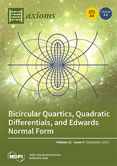
The structure of cubic plane curves is governed by lines. Likewise, circle geometry underlies the theory of bicircular quartics. Such a quartic is symmetric in four mutually orthogonal circles of inversion; its sixteen (complex) foci lie on the latter and the curve belongs to an orthogonal family of such quartics sharing the same circles and foci. Here, we connect the above geometric setting with the normal form for elliptic curves introduced by Edwards in 2007. Each (real) Edwards curve generates a confocal family of equivalent elliptic curves—bicircular quartics—via a parameterized Edwards transformation. Curves in the family are identified with trajectories of a quadratic differential on the Riemann sphere. In combination, these several topics illuminate each other and facilitate our fuller understanding of them. View this paper
  • Issues are regarded as officially published after their release is announced to the table of contents alert mailing list.
  • You may sign up for e-mail alerts to receive table of contents of newly released issues.
  • PDF is the official format for papers published in both, html and pdf forms. To view the papers in pdf format, click on the "PDF Full-text" link, and use the free Adobe Reader to open them.
Order results
Result details
Section
Select all
Export citation of selected articles as:
17 pages, 643 KiB  
Article
On the Modified Numerical Methods for Partial Differential Equations Involving Fractional Derivatives
by Fahad Alsidrani, Adem Kılıçman and Norazak Senu
Axioms 2023, 12(9), 901; https://doi.org/10.3390/axioms12090901 - 21 Sep 2023
Viewed by 1552
Abstract
This paper provides both analytical and numerical solutions of (PDEs) involving time-fractional derivatives. We implemented three powerful techniques, including the modified variational iteration technique, the modified Adomian decomposition technique, and the modified homotopy analysis technique, to obtain an approximate solution for the bounded [...] Read more.
This paper provides both analytical and numerical solutions of (PDEs) involving time-fractional derivatives. We implemented three powerful techniques, including the modified variational iteration technique, the modified Adomian decomposition technique, and the modified homotopy analysis technique, to obtain an approximate solution for the bounded space variable ν. The Laplace transformation is used in the time-fractional derivative operator to enhance the proposed numerical methods’ performance and accuracy and find an approximate solution to time-fractional Fornberg–Whitham equations. To confirm the accuracy of the proposed methods, we evaluate homogeneous time-fractional Fornberg–Whitham equations in terms of non-integer order and variable coefficients. The obtained results of the modified methods are shown through tables and graphs. Full article
Show Figures

Figure 1

Figure 1
<p>(<b>a</b>) Three-dimensional surface for <math display="inline"><semantics> <mfenced separators="" open="|" close="|"> <mi>E</mi> <mi>x</mi> <mi>a</mi> <mi>c</mi> <mi>t</mi> <mo>−</mo> <mi mathvariant="sans-serif">ψ</mi> <mo>(</mo> <mi>ν</mi> <mo>,</mo> <mi>ς</mi> <mo>)</mo> </mfenced> </semantics></math> of LVIM Equation (58) at <math display="inline"><semantics> <mrow> <mi>ϑ</mi> <mo>=</mo> <mn>0.15</mn> </mrow> </semantics></math>; (<b>b</b>) surface for <math display="inline"><semantics> <mfenced separators="" open="|" close="|"> <mi>E</mi> <mi>x</mi> <mi>a</mi> <mi>c</mi> <mi>t</mi> <mo>−</mo> <mi mathvariant="sans-serif">ψ</mi> <mo>(</mo> <mi>ν</mi> <mo>,</mo> <mi>ς</mi> <mo>)</mo> </mfenced> </semantics></math> of LVIM Equation (58) at <math display="inline"><semantics> <mrow> <mi>ϑ</mi> <mo>=</mo> <mn>0.5</mn> </mrow> </semantics></math>; (<b>c</b>) two-dimensional plots for <math display="inline"><semantics> <mfenced separators="" open="|" close="|"> <mi>E</mi> <mi>x</mi> <mi>a</mi> <mi>c</mi> <mi>t</mi> <mo>−</mo> <mi mathvariant="sans-serif">ψ</mi> <mo>(</mo> <mi>ν</mi> <mo>,</mo> <mi>ς</mi> <mo>)</mo> </mfenced> </semantics></math> of LVIM Equation (58) with respect to <math display="inline"><semantics> <mrow> <mi>ς</mi> <mo>=</mo> <mn>1</mn> </mrow> </semantics></math> at different values of <math display="inline"><semantics> <mi>ϑ</mi> </semantics></math> in Example 1.</p>
Full article ">Figure 2
<p>(<b>a</b>) Three-dimensional surface for <math display="inline"><semantics> <mfenced separators="" open="|" close="|"> <mi>E</mi> <mi>x</mi> <mi>a</mi> <mi>c</mi> <mi>t</mi> <mo>−</mo> <mi mathvariant="sans-serif">ψ</mi> <mo>(</mo> <mi>ν</mi> <mo>,</mo> <mi>ς</mi> <mo>)</mo> </mfenced> </semantics></math> of LADM Equation (66) at <math display="inline"><semantics> <mrow> <mi>ϑ</mi> <mo>=</mo> <mn>0.15</mn> </mrow> </semantics></math>; (<b>b</b>) surface for <math display="inline"><semantics> <mfenced separators="" open="|" close="|"> <mi>E</mi> <mi>x</mi> <mi>a</mi> <mi>c</mi> <mi>t</mi> <mo>−</mo> <mi mathvariant="sans-serif">ψ</mi> <mo>(</mo> <mi>ν</mi> <mo>,</mo> <mi>ς</mi> <mo>)</mo> </mfenced> </semantics></math> of LADM Equation (66) at <math display="inline"><semantics> <mrow> <mi>ϑ</mi> <mo>=</mo> <mn>0.5</mn> </mrow> </semantics></math>; (<b>c</b>) two-dimensional plots for <math display="inline"><semantics> <mfenced separators="" open="|" close="|"> <mi>E</mi> <mi>x</mi> <mi>a</mi> <mi>c</mi> <mi>t</mi> <mo>−</mo> <mi mathvariant="sans-serif">ψ</mi> <mo>(</mo> <mi>ν</mi> <mo>,</mo> <mi>ς</mi> <mo>)</mo> </mfenced> </semantics></math> of LADM Equation (66) with respect to <math display="inline"><semantics> <mrow> <mi>ς</mi> <mo>=</mo> <mn>1</mn> </mrow> </semantics></math> at different values of <math display="inline"><semantics> <mi>ϑ</mi> </semantics></math> in Example 1.</p>
Full article ">Figure 3
<p>(<b>a</b>) Three-dimensional surface for <math display="inline"><semantics> <mfenced separators="" open="|" close="|"> <mi>E</mi> <mi>x</mi> <mi>a</mi> <mi>c</mi> <mi>t</mi> <mo>−</mo> <mi mathvariant="sans-serif">ψ</mi> <mo>(</mo> <mi>ν</mi> <mo>,</mo> <mi>ς</mi> <mo>)</mo> </mfenced> </semantics></math> of LHAM Equation (77) at <math display="inline"><semantics> <mrow> <mi>ϑ</mi> <mo>=</mo> <mn>0.15</mn> </mrow> </semantics></math>, <math display="inline"><semantics> <mrow> <mo>ℏ</mo> <mo>=</mo> <mo>−</mo> <mn>0.0001</mn> </mrow> </semantics></math>, and <math display="inline"><semantics> <mrow> <mi>n</mi> <mo>=</mo> <mn>1</mn> </mrow> </semantics></math>; (<b>b</b>) surface for <math display="inline"><semantics> <mfenced separators="" open="|" close="|"> <mi>E</mi> <mi>x</mi> <mi>a</mi> <mi>c</mi> <mi>t</mi> <mo>−</mo> <mi mathvariant="sans-serif">ψ</mi> <mo>(</mo> <mi>ν</mi> <mo>,</mo> <mi>ς</mi> <mo>)</mo> </mfenced> </semantics></math> of LHAM Equation (77) at <math display="inline"><semantics> <mrow> <mi>ϑ</mi> <mo>=</mo> <mn>0.5</mn> </mrow> </semantics></math>, <math display="inline"><semantics> <mrow> <mo>ℏ</mo> <mo>=</mo> <mo>−</mo> <mn>0.0001</mn> </mrow> </semantics></math>, and <math display="inline"><semantics> <mrow> <mi>n</mi> <mo>=</mo> <mn>1</mn> </mrow> </semantics></math>; (<b>c</b>) two-dimensional plots for <math display="inline"><semantics> <mfenced separators="" open="|" close="|"> <mi>E</mi> <mi>x</mi> <mi>a</mi> <mi>c</mi> <mi>t</mi> <mo>−</mo> <mi mathvariant="sans-serif">ψ</mi> <mo>(</mo> <mi>ν</mi> <mo>,</mo> <mi>ς</mi> <mo>)</mo> </mfenced> </semantics></math> of LHAM Equation (77) with respect to <math display="inline"><semantics> <mrow> <mi>ς</mi> <mo>=</mo> <mn>1</mn> </mrow> </semantics></math>, <math display="inline"><semantics> <mrow> <mo>ℏ</mo> <mo>=</mo> <mo>−</mo> <mn>0.0001</mn> </mrow> </semantics></math>, and <math display="inline"><semantics> <mrow> <mi>n</mi> <mo>=</mo> <mn>1</mn> </mrow> </semantics></math> at different values of <math display="inline"><semantics> <mi>ϑ</mi> </semantics></math> in Example 1.</p>
Full article ">
20 pages, 6303 KiB  
Article
Optimizing Port Multi-AGV Trajectory Planning through Priority Coordination: Enhancing Efficiency and Safety
by Yongjun Chen, Shuquan Shi, Zong Chen, Tengfei Wang, Longkun Miao and Huiting Song
Axioms 2023, 12(9), 900; https://doi.org/10.3390/axioms12090900 - 21 Sep 2023
Viewed by 1371
Abstract
Efficient logistics and transport at the port heavily relies on efficient AGV scheduling and planning for container transshipment. This paper presents a comprehensive approach to address the challenges in AGV path planning and coordination within the domain of intelligent transportation systems. We propose [...] Read more.
Efficient logistics and transport at the port heavily relies on efficient AGV scheduling and planning for container transshipment. This paper presents a comprehensive approach to address the challenges in AGV path planning and coordination within the domain of intelligent transportation systems. We propose an enhanced graph search method for constructing the global path of a single AGV that mitigates the issues associated with paths closely aligned with obstacle corner points. Moreover, a centralized global planning module is developed to facilitate planning and scheduling. Each individual AGV establishes real-time communication with the upper layers to accurately determine its position at complex intersections. By computing its priority sequence within a coordination circle, the AGV effectively treats the high-priority trajectories of other vehicles as dynamic obstacles for its local trajectory planning. The feasibility of trajectory information is ensured by solving the online real-time Optimal Control Problem (OCP). In the trajectory planning process for a single AGV, we incorporate a linear programming-based obstacle avoidance strategy. This strategy transforms the obstacle avoidance optimization problem into trajectory planning constraints using Karush-Kuhn-Tucker (KKT) conditions. Consequently, seamless and secure AGV movement within the port environment is guaranteed. The global planning module encompasses a global regulatory mechanism that provides each AGV with an initial feasible path. This approach not only facilitates complexity decomposition for large-scale problems, but also maintains path feasibility through continuous real-time communication with the upper layers during AGV travel. A key advantage of our progressive solution lies in its flexibility and scalability. This approach readily accommodates extensions based on the original problem and allows adjustments in the overall problem size in response to varying port cargo throughput, all without requiring a complete system overhaul. Full article
(This article belongs to the Special Issue Mathematical Modelling of Complex Systems)
Show Figures

Figure 1

Figure 1
<p>Illustration of the path generated by RRT* (<b>left</b>), where the red line represents the path generated by the RRT* algorithm, while the blue lines represent the branches of the exploring random tree. The red points indicate the random sampling points used in the algorithm, (<b>right</b>) Voronoi Graph, the yellow lines represent the feasible edges generated by the Voronoi Graph, while the red points indicate the obstacles in the environment.</p>
Full article ">Figure 2
<p>Illustration of the Path that generated by the A* algorithm (<b>left</b>) and Augmented Graph Search (<b>right</b>). Where the blue star and red cross demonstrate the start and goal point, respectively. and the black line (<b>left</b>) and the thin blue line (<b>right</b>) are the result of the A* algorithm, the red line is the result of the enhanced graph search, and the black dots are the virtual obstacles added in the enhanced graph search.</p>
Full article ">Figure 3
<p>Illustration of Augmented Graph-search-based Motion Planning Framework.</p>
Full article ">Figure 4
<p>Illustration of pose variables of the Robot.</p>
Full article ">Figure 5
<p>Illustration of the Path that generated by the A* algorithm in Rviz. Where the blue and red arrow demonstrate the start and goal pose.</p>
Full article ">Figure 6
<p>Illustration that collision happens during the interval [<math display="inline"><semantics> <msub> <mi>t</mi> <mi>j</mi> </msub> </semantics></math>,<math display="inline"><semantics> <msub> <mi>t</mi> <mrow> <mi>j</mi> <mo>+</mo> <mn>1</mn> </mrow> </msub> </semantics></math>]. We add new fit point <math display="inline"><semantics> <mrow> <msub> <mi>t</mi> <msup> <mi>j</mi> <mo>′</mo> </msup> </msub> <mo>∈</mo> <mrow> <mo>[</mo> <msub> <mi>t</mi> <mi>j</mi> </msub> <mo>,</mo> <msub> <mi>t</mi> <mrow> <mi>j</mi> <mo>+</mo> <mn>1</mn> </mrow> </msub> <mo>]</mo> </mrow> </mrow> </semantics></math>, and modified spline is collision free in [<math display="inline"><semantics> <msub> <mi>t</mi> <mi>j</mi> </msub> </semantics></math>,<math display="inline"><semantics> <msub> <mi>t</mi> <mrow> <mi>j</mi> <mo>+</mo> <mn>1</mn> </mrow> </msub> </semantics></math>].</p>
Full article ">Figure 7
<p>Illustration of collision avoidance of two convex polygons <math display="inline"><semantics> <mi mathvariant="script">M</mi> </semantics></math> and <math display="inline"><semantics> <mi mathvariant="script">N</mi> </semantics></math>.</p>
Full article ">Figure 8
<p>Illustration of numerical simulation of obstacle avoidance using J-function under rectangular obstacle.</p>
Full article ">Figure 9
<p>Illustration of numerical simulation of obstacle avoidance using J-function under circle obstacles.</p>
Full article ">Figure 10
<p>Variation curve of heading angle <math display="inline"><semantics> <mi>θ</mi> </semantics></math> with time <span class="html-italic">s</span> with J obstacle avoidance. (<b>a</b>) Rectangle collision avoidance. (<b>b</b>) Circle collision avoidance.</p>
Full article ">Figure 11
<p>Simulation in S and L environments was conducted under Gazebo. The static obstacle is a wall, and cuboids and spheres were randomly added as dynamic obstacles.</p>
Full article ">Figure 12
<p>Simulation in S and L environments using Rviz, where the green lines represent the global paths and the red lines represent the actual tracking trajectories produced by the warehouse model.</p>
Full article ">Figure 13
<p>Port overview scenes. Where the black block demonstrate the container yard, the shadow blue circle is the coordinate circle, the dark blue block represents the container ship berth, the gap in the upper right corner is the exit from the port area.</p>
Full article ">Figure 14
<p>Multi AGVs coordinate transportation in port scenes.</p>
Full article ">Figure 15
<p>Comparison of our proposed method and coupled method [<a href="#B51-axioms-12-00900" class="html-bibr">51</a>] and the total time in global planning. (<b>a</b>) Comparison of our method and coupled method. (<b>b</b>) Total planning and Enhanced graph search time.</p>
Full article ">Figure 16
<p>Multi AGVs coordinate transportation in double intersections scenes.</p>
Full article ">
13 pages, 311 KiB  
Article
Cumulative Entropy of Past Lifetime for Coherent Systems at the System Level
by Mansour Shrahili and Mohamed Kayid
Axioms 2023, 12(9), 899; https://doi.org/10.3390/axioms12090899 - 21 Sep 2023
Viewed by 910
Abstract
This paper explores the cumulative entropy of the lifetime of an n-component coherent system, given the precondition that all system components have experienced failure at time t. This investigation utilizes the system signature to compute the cumulative entropy of the system’s [...] Read more.
This paper explores the cumulative entropy of the lifetime of an n-component coherent system, given the precondition that all system components have experienced failure at time t. This investigation utilizes the system signature to compute the cumulative entropy of the system’s lifetime, shedding light on a crucial facet of a system’s predictability. In the course of this research, we unearth a series of noteworthy discoveries. These include formulating expressions, defining bounds, and identifying orderings related to this measure. Further, we propose a technique to identify a preferred system on the basis of cumulative Kullback–Leibler discriminating information, which exhibits a strong relation with the parallel system. These findings contribute significantly to our understanding of the predictability of a coherent system’s lifetime, underscoring the importance of this field of study. The outcomes offer potential benefits for a wide range of applications where system predictability is paramount, and where the comparative evaluation of different systems on the basis of discriminating information is needed. Full article
Show Figures

Figure 1

Figure 1
<p>A coherent system with signature <math display="inline"><semantics> <mi mathvariant="bold">p</mi> </semantics></math> = <math display="inline"><semantics> <mrow> <mo>(</mo> <mn>0</mn> <mo>,</mo> <mo> </mo> <mn>4</mn> <mo>/</mo> <mn>45</mn> <mo>,</mo> <mo> </mo> <mn>19</mn> <mo>/</mo> <mn>90</mn> <mo>,</mo> <mo> </mo> <mn>3</mn> <mo>/</mo> <mn>10</mn> <mo>,</mo> <mo> </mo> <mn>86</mn> <mo>/</mo> <mn>315</mn> <mo>,</mo> <mo> </mo> <mn>34</mn> <mo>/</mo> <mn>315</mn> <mo>,</mo> <mo> </mo> <mn>2</mn> <mo>/</mo> <mn>105</mn> <mo>,</mo> <mo> </mo> <mn>0</mn> <mo>,</mo> <mo> </mo> <mn>0</mn> <mo>,</mo> <mo> </mo> <mn>0</mn> <mo>)</mo> </mrow> </semantics></math>.</p>
Full article ">Figure 2
<p>Cumulative entropy of <math display="inline"><semantics> <msub> <mi>T</mi> <mi>t</mi> </msub> </semantics></math> with respect to <span class="html-italic">t</span> for various values of <math display="inline"><semantics> <mrow> <mi>k</mi> <mo>&gt;</mo> <mn>0</mn> </mrow> </semantics></math>, using the cdf Part (ii) from Example 1.</p>
Full article ">
15 pages, 337 KiB  
Article
Sinc Collocation Method to Simulate the Fractional Partial Integro-Differential Equation with a Weakly Singular Kernel
by Mingzhu Li, Lijuan Chen and Yongtao Zhou
Axioms 2023, 12(9), 898; https://doi.org/10.3390/axioms12090898 - 21 Sep 2023
Cited by 1 | Viewed by 976
Abstract
In this article, we develop an efficient numerical scheme for dealing with fractional partial integro-differential equations (FPIEs) with a weakly singular kernel. The weight and shift Grünwald difference (WSGD) operator is adopted to approximate a time fractional derivative and the Sinc collocation method [...] Read more.
In this article, we develop an efficient numerical scheme for dealing with fractional partial integro-differential equations (FPIEs) with a weakly singular kernel. The weight and shift Grünwald difference (WSGD) operator is adopted to approximate a time fractional derivative and the Sinc collocation method is applied for discretizing the spatial derivative.The exponential convergence of our proposed method is demonstrated in detail. Finally, numerical evidence is employed to verify the theoretical results and confirm the expected convergence rate. Full article
(This article belongs to the Special Issue Differential Equations and Inverse Problems)
Show Figures

Figure 1

Figure 1
<p>The maximum norm errors with <math display="inline"><semantics> <mrow> <mi>α</mi> <mo>=</mo> <mn>0.8</mn> </mrow> </semantics></math> and <math display="inline"><semantics> <mrow> <mi>τ</mi> <mo>=</mo> <mfrac> <mn>1</mn> <mn>1000</mn> </mfrac> </mrow> </semantics></math>.</p>
Full article ">Figure 2
<p>The maximum norm errors with <math display="inline"><semantics> <mrow> <mi>α</mi> <mo>=</mo> <mn>0.4</mn> </mrow> </semantics></math> and <math display="inline"><semantics> <mrow> <mi>τ</mi> <mo>=</mo> <mfrac> <mn>1</mn> <mn>512</mn> </mfrac> </mrow> </semantics></math>.</p>
Full article ">Figure 3
<p>Numerical solution and analytical solution with <math display="inline"><semantics> <mrow> <mi>α</mi> <mo>=</mo> <mn>0.5</mn> </mrow> </semantics></math>, <math display="inline"><semantics> <mrow> <mi>τ</mi> <mo>=</mo> <mfrac> <mn>1</mn> <mn>512</mn> </mfrac> </mrow> </semantics></math> and <math display="inline"><semantics> <mrow> <mi>N</mi> <mo>=</mo> <mn>64</mn> </mrow> </semantics></math>.</p>
Full article ">
13 pages, 332 KiB  
Article
A Two-Step Newton Algorithm for the Weighted Complementarity Problem with Local Biquadratic Convergence
by Xiangjing Liu, Yihan Liu and Jianke Zhang
Axioms 2023, 12(9), 897; https://doi.org/10.3390/axioms12090897 - 20 Sep 2023
Cited by 1 | Viewed by 971
Abstract
We discuss the weighted complementarity problem, extending the nonlinear complementarity problem on Rn. In contrast to the NCP, many equilibrium problems in science, engineering, and economics can be transformed into WCPs for more efficient methods. Smoothing Newton algorithms, known for their [...] Read more.
We discuss the weighted complementarity problem, extending the nonlinear complementarity problem on Rn. In contrast to the NCP, many equilibrium problems in science, engineering, and economics can be transformed into WCPs for more efficient methods. Smoothing Newton algorithms, known for their at least locally superlinear convergence properties, have been widely applied to solve WCPs. We suggest a two-step Newton approach with a local biquadratic order convergence rate to solve the WCP. The new method needs to calculate two Newton equations at each iteration. We also insert a new term, which is of crucial importance for the local biquadratic convergence properties when solving the Newton equation. We demonstrate that the solution to the WCP is the accumulation point of the iterative sequence produced by the approach. We further demonstrate that the algorithm possesses local biquadratic convergence properties. Numerical results indicate the method to be practical and efficient. Full article
(This article belongs to the Special Issue Computational Mathematics in Engineering and Applied Science)
12 pages, 295 KiB  
Article
Almost Boyd-Wong Type Contractions under Binary Relations with Applications to Boundary Value Problems
by Amal F. Alharbi and Faizan Ahmad Khan
Axioms 2023, 12(9), 896; https://doi.org/10.3390/axioms12090896 - 20 Sep 2023
Cited by 2 | Viewed by 827
Abstract
This article is devoted to investigating the fixed point theorems for a new contracitivity contraction, which combines the idea involved in Boyd-Wong contractions, strict almost contractions and relational contractions. Our results improve and expand existing fixed point theorems of literature. In process, we [...] Read more.
This article is devoted to investigating the fixed point theorems for a new contracitivity contraction, which combines the idea involved in Boyd-Wong contractions, strict almost contractions and relational contractions. Our results improve and expand existing fixed point theorems of literature. In process, we deduce a metrical fixed point theorem for strict almost Boyd-Wong contractions. To demonstrate the credibility of our results, we present a number of a few examples. Applying our findings, we find a unique solution to a particular periodic boundary value problem. Full article
(This article belongs to the Special Issue Fixed Point Theory and Its Related Topics IV)
15 pages, 692 KiB  
Article
New Results Achieved for Fractional Differential Equations with Riemann–Liouville Derivatives of Nonlinear Variable Order
by Hallouz Abdelhamid, Gani Stamov, Mohammed Said Souid and Ivanka Stamova
Axioms 2023, 12(9), 895; https://doi.org/10.3390/axioms12090895 - 20 Sep 2023
Cited by 2 | Viewed by 1072
Abstract
This paper proposes new existence and uniqueness results for an initial value problem (IVP) of fractional differential equations of nonlinear variable order. Riemann–Liouville-type fractional derivatives are considered in the problem. The new fundamental results achieved in this work are obtained by using the [...] Read more.
This paper proposes new existence and uniqueness results for an initial value problem (IVP) of fractional differential equations of nonlinear variable order. Riemann–Liouville-type fractional derivatives are considered in the problem. The new fundamental results achieved in this work are obtained by using the inequalities technique and the fixed point theory. In addition, uniform stability criteria for the solutions are derived. The accomplished results are new and complement the scientific research in the field. A numerical example is composed to show the efficacy and potency of the proposed criteria. Full article
(This article belongs to the Special Issue Fractional Calculus and the Applied Analysis)
Show Figures

Figure 1

Figure 1
<p>The approximate solution <math display="inline"><semantics> <mrow> <mi>y</mi> <mo>(</mo> <mi>t</mi> <mo>)</mo> </mrow> </semantics></math> in <math display="inline"><semantics> <mrow> <mo>[</mo> <mn>0</mn> <mo>,</mo> <mn>1</mn> <mo>]</mo> </mrow> </semantics></math> with <math display="inline"><semantics> <mrow> <mi>β</mi> <mrow> <mo>(</mo> <mi>t</mi> <mo>,</mo> <mi>y</mi> <mo>)</mo> </mrow> <mo>=</mo> <mfrac> <msup> <mi>t</mi> <mn>3</mn> </msup> <mn>3</mn> </mfrac> <mo>+</mo> <mfrac> <mi>t</mi> <mn>3</mn> </mfrac> <mo>+</mo> <mfrac> <mn>1</mn> <mrow> <mn>3</mn> <mo>(</mo> <msup> <mi>y</mi> <mn>2</mn> </msup> <mo>+</mo> <mn>1</mn> <mo>)</mo> </mrow> </mfrac> </mrow> </semantics></math>.</p>
Full article ">Figure 2
<p>The function <math display="inline"><semantics> <mrow> <mi>β</mi> <mo>(</mo> <mi>t</mi> <mo>,</mo> <mi>y</mi> <mo>)</mo> </mrow> </semantics></math> for <math display="inline"><semantics> <mrow> <mi>t</mi> <mo>∈</mo> <mo>[</mo> <mn>0</mn> <mo>,</mo> <mn>1</mn> <mo>]</mo> </mrow> </semantics></math> and <math display="inline"><semantics> <mrow> <mi>y</mi> <mo>∈</mo> <mo>[</mo> <mn>0</mn> <mo>,</mo> <mn>20</mn> <mo>]</mo> </mrow> </semantics></math>.</p>
Full article ">Figure 3
<p>The function <math display="inline"><semantics> <mrow> <mi>ψ</mi> <mo>(</mo> <mi>t</mi> <mo>,</mo> <mi>y</mi> <mo>)</mo> </mrow> </semantics></math> for <math display="inline"><semantics> <mrow> <mi>t</mi> <mo>∈</mo> <mo>[</mo> <mn>0</mn> <mo>,</mo> <mn>1</mn> <mo>]</mo> </mrow> </semantics></math> and <math display="inline"><semantics> <mrow> <mi>y</mi> <mo>∈</mo> <mo>[</mo> <mn>0</mn> <mo>,</mo> <mn>20</mn> <mo>]</mo> </mrow> </semantics></math>.</p>
Full article ">
16 pages, 463 KiB  
Article
A Least Squares Estimator for Gradual Change-Point in Time Series with m-Asymptotically Almost Negatively Associated Errors
by Tianming Xu and Yuesong Wei
Axioms 2023, 12(9), 894; https://doi.org/10.3390/axioms12090894 - 20 Sep 2023
Viewed by 818
Abstract
As a new member of the NA (negative associated) family, the m-AANA (m-asymptotically almost negatively associated) sequence has many statistical properties that have not been developed. This paper mainly studies its properties in the gradual change point model. Firstly, we [...] Read more.
As a new member of the NA (negative associated) family, the m-AANA (m-asymptotically almost negatively associated) sequence has many statistical properties that have not been developed. This paper mainly studies its properties in the gradual change point model. Firstly, we propose a least squares type change point estimator, then derive the convergence rates and consistency of the estimator, and provide the limit distributions of the estimator. It is interesting that the convergence rates of the estimator are the same as that of the change point estimator for independent identically distributed observations. Finally, the effectiveness of the estimator in limited samples can be verified through several sets of simulation experiments and an actual hydrological example. Full article
(This article belongs to the Special Issue Probability, Statistics and Estimation)
Show Figures

Figure 1

Figure 1
<p>The box plots of <math display="inline"><semantics> <mrow> <msup> <mover accent="true"> <mi>τ</mi> <mo stretchy="false">^</mo> </mover> <mo>*</mo> </msup> <mo>−</mo> <msup> <mi>τ</mi> <mo>*</mo> </msup> </mrow> </semantics></math> with <math display="inline"><semantics> <mrow> <mi>γ</mi> <mo>=</mo> <mn>0.75</mn> </mrow> </semantics></math>, <math display="inline"><semantics> <mrow> <msub> <mi>δ</mi> <mi>n</mi> </msub> <mo>=</mo> <msup> <mi>n</mi> <mrow> <mo>−</mo> <mn>0.1</mn> </mrow> </msup> <mo>,</mo> <mn>1</mn> <mo>,</mo> <msup> <mi>n</mi> <mrow> <mn>0.1</mn> </mrow> </msup> <mo>,</mo> <msup> <mi>n</mi> <mrow> <mn>0.2</mn> </mrow> </msup> <mo>,</mo> </mrow> </semantics></math> and <math display="inline"><semantics> <mrow> <msup> <mi>τ</mi> <mo>*</mo> </msup> <mo>=</mo> <mn>1</mn> <mo>/</mo> <mn>2</mn> </mrow> </semantics></math>.</p>
Full article ">Figure 2
<p>The box plots of <math display="inline"><semantics> <mrow> <msup> <mover accent="true"> <mi>τ</mi> <mo stretchy="false">^</mo> </mover> <mo>*</mo> </msup> <mo>−</mo> <msup> <mi>τ</mi> <mo>*</mo> </msup> </mrow> </semantics></math> with <math display="inline"><semantics> <mrow> <mi>γ</mi> <mo>=</mo> <mn>0.5</mn> </mrow> </semantics></math>, <math display="inline"><semantics> <mrow> <msub> <mi>δ</mi> <mi>n</mi> </msub> <mo>=</mo> <msup> <mi>n</mi> <mrow> <mo>−</mo> <mn>0.1</mn> </mrow> </msup> <mo>,</mo> <mn>1</mn> <mo>,</mo> <msup> <mi>n</mi> <mrow> <mn>0.1</mn> </mrow> </msup> <mo>,</mo> <msup> <mi>n</mi> <mrow> <mn>0.2</mn> </mrow> </msup> <mo>,</mo> </mrow> </semantics></math> and <math display="inline"><semantics> <mrow> <msup> <mi>τ</mi> <mo>*</mo> </msup> <mo>=</mo> <mn>1</mn> <mo>/</mo> <mn>2</mn> </mrow> </semantics></math>.</p>
Full article ">Figure 3
<p>The box plots of <math display="inline"><semantics> <mrow> <msup> <mover accent="true"> <mi>τ</mi> <mo stretchy="false">^</mo> </mover> <mo>*</mo> </msup> <mo>−</mo> <msup> <mi>τ</mi> <mo>*</mo> </msup> </mrow> </semantics></math> with <math display="inline"><semantics> <mrow> <mi>γ</mi> <mo>=</mo> <mn>0.25</mn> </mrow> </semantics></math>, <math display="inline"><semantics> <mrow> <msub> <mi>δ</mi> <mi>n</mi> </msub> <mo>=</mo> <msup> <mi>n</mi> <mrow> <mo>−</mo> <mn>0.1</mn> </mrow> </msup> <mo>,</mo> <mn>1</mn> <mo>,</mo> <msup> <mi>n</mi> <mrow> <mn>0.1</mn> </mrow> </msup> <mo>,</mo> <msup> <mi>n</mi> <mrow> <mn>0.2</mn> </mrow> </msup> <mo>,</mo> </mrow> </semantics></math> and <math display="inline"><semantics> <mrow> <msup> <mi>τ</mi> <mo>*</mo> </msup> <mo>=</mo> <mn>1</mn> <mo>/</mo> <mn>2</mn> </mrow> </semantics></math>.</p>
Full article ">Figure 4
<p>The plot graph of monthly average water levels of Hulun Lake from 1992 to 2008.</p>
Full article ">Figure 5
<p>Autocorrelation function.</p>
Full article ">
15 pages, 813 KiB  
Article
Minor and Major Strain: Equations of Equilibrium of a Plane Domain with an Angular Cutout in the Boundary
by Lyudmila Frishter
Axioms 2023, 12(9), 893; https://doi.org/10.3390/axioms12090893 - 19 Sep 2023
Viewed by 998
Abstract
Large values and gradients of stress and strain, triggering concentrated stress and strain, arise in angular areas of a structure. The strain action, leading to the finite loss of contact between structural elements, also triggers concentrated stress. The loss of contact reaches an [...] Read more.
Large values and gradients of stress and strain, triggering concentrated stress and strain, arise in angular areas of a structure. The strain action, leading to the finite loss of contact between structural elements, also triggers concentrated stress. The loss of contact reaches an irregular point and a line on the boundary. The theoretical analysis of the stress–strain state (SSS) of areas with angular cutouts in the boundary under the action of discontinuous strain is reduced to the study of singular solutions to the homogeneous problem of elasticity theory with power-related features. The calculation of stress concentration coefficients in the domain of a singular solution to the elastic problem makes no sense. It is experimentally proven that the area located near the vertex of an angular cutout in the boundary features substantial strain and rotations, and it corresponds to higher values of the first and second derivatives of displacements along the radius in cases of sufficiently small radii in the neighborhood of an irregular boundary point. As far as these areas are concerned, it is necessary to consider the plane problem of the elasticity theory, taking into account the geometric nonlinearity under the action of strain, to analyze the effect of relationships between strain orders, rotations, and strain on the form of the equation of equilibrium. The purpose of this work is to analyze the effect of relationships between strain orders, rotations, and strain on the form of the equilibrium equation in the polar system of coordinates for a V-shaped area under the action of temperature-induced strain, taking into account geometric non-linearity and physical linearity. Full article
(This article belongs to the Special Issue Applied Numerical Analysis in Civil Engineering)
Show Figures

Figure 1

Figure 1
<p>Interference fringes for a plane model with 90° and 60° angles of the cutout and temperature-induced model strain.</p>
Full article ">Figure 2
<p>Plane V-shaped domain <math display="inline"><semantics> <mi mathvariant="sans-serif">Ω</mi> </semantics></math>.</p>
Full article ">
14 pages, 3715 KiB  
Article
Synergy Prediction Model of Information Entropy Based on Zone Safety Degree and Stope Roof Weighting Step Analysis
by Lijun Xiong, Haiping Yuan, Hengzhe Li, Xiaohu Liu, Yangyao Zou, Shuaijie Ji and Xingye Fang
Axioms 2023, 12(9), 892; https://doi.org/10.3390/axioms12090892 - 19 Sep 2023
Cited by 1 | Viewed by 834
Abstract
During the underground mining of coal resources, the rock pressure emerges acutely and the mine geological disasters occur frequently. It is of great significance to grasp the manifestation law of rock pressure in time to guide the safety production and operation in the [...] Read more.
During the underground mining of coal resources, the rock pressure emerges acutely and the mine geological disasters occur frequently. It is of great significance to grasp the manifestation law of rock pressure in time to guide the safety production and operation in the pit. In this research, the calculation equations and concept of information entropy based on zone safety degree are primarily defined, and the synergetic theory of the maximum information entropy principle is combined to put forward the synergy prediction model of information entropy based on zone safety degree. In the meantime, the synergy prediction model of information entropy based on zone safety degree is employed to calculate and predict the first weighting step and the periodic weighting step of the main roof of the 9203 working face of Hengsheng Coal Mine in China’s Shanxi Province, as well as verifying the validity and reliability of the synergy prediction model of information entropy based on zone safety degree by the comparison of similar simulation test results, which has presented a scientific basis for the effective control of rock pressure and roof management. Full article
Show Figures

Figure 1

Figure 1
<p>Mohr-Coulomb strength criterion.</p>
Full article ">Figure 2
<p>Integrated histogram of coal and rock strata.</p>
Full article ">Figure 3
<p>Geometrical model.</p>
Full article ">Figure 4
<p>Prediction flow chart of weighting step of the 9203 working face roof.</p>
Full article ">Figure 5
<p>Cloud diagram of zone safety degree in elastoplastic critical states.</p>
Full article ">Figure 6
<p>Prediction curve of weighting step of main roof.</p>
Full article ">
27 pages, 551 KiB  
Article
Ninth-order Multistep Collocation Formulas for Solving Models of PDEs Arising in Fluid Dynamics: Design and Implementation Strategies
by Ezekiel Olaoluwa Omole, Emmanuel Oluseye Adeyefa, Victoria Iyadunni Ayodele, Ali Shokri and Yuanheng Wang
Axioms 2023, 12(9), 891; https://doi.org/10.3390/axioms12090891 - 18 Sep 2023
Cited by 11 | Viewed by 1019
Abstract
A computational approach with the aid of the Linear Multistep Method (LMM) for the numerical solution of differential equations with initial value problems or boundary conditions has appeared several times in the literature due to its good accuracy and stability properties. The major [...] Read more.
A computational approach with the aid of the Linear Multistep Method (LMM) for the numerical solution of differential equations with initial value problems or boundary conditions has appeared several times in the literature due to its good accuracy and stability properties. The major objective of this article is to extend a multistep approach for the numerical solution of the Partial Differential Equation (PDE) originating from fluid mechanics in a two-dimensional space with initial and boundary conditions, as a result of the importance and utility of the models of partial differential equations in applications, particularly in physical phenomena, such as in convection-diffusion models, and fluid flow problems. Thus, a multistep collocation formula, which is based on orthogonal polynomials is proposed. Ninth-order Multistep Collocation Formulas (NMCFs) were formulated through the principle of interpolation and collocation processes. The theoretical analysis of the NMCFs reveals that they have algebraic order nine, are zero-stable, consistent, and, thus, convergent. The implementation strategies of the NMCFs are comprehensively discussed. Some numerical test problems were presented to evaluate the efficacy and applicability of the proposed formulas. Comparisons with other methods were also presented to demonstrate the new formulas’ productivity. Finally, figures were presented to illustrate the behavior of the numerical examples. Full article
(This article belongs to the Special Issue Differential Equations and Related Topics)
Show Figures

Figure 1

Figure 1
<p>Region of absolute stability of the NMCFs.</p>
Full article ">Figure 2
<p>Comparison of errors in NMCFs versus Yagider and Karabacak [<a href="#B44-axioms-12-00891" class="html-bibr">44</a>] for test problem 5.1.</p>
Full article ">Figure 3
<p>Comparison of errors in NMCFs versus Lima et al. [<a href="#B45-axioms-12-00891" class="html-bibr">45</a>] for test problem 5.2.</p>
Full article ">Figure 4
<p>Comparison of errors in NMCFs versus Lima et al. [<a href="#B45-axioms-12-00891" class="html-bibr">45</a>] for test problem 5.3.</p>
Full article ">Figure 5
<p>Comparison of errors in NMCFs versus Biala et al. [<a href="#B46-axioms-12-00891" class="html-bibr">46</a>] and Xu and Wang [<a href="#B47-axioms-12-00891" class="html-bibr">47</a>] for test problem 5.4.</p>
Full article ">Figure 6
<p>Comparison of errors in NMCFs versus Biala and Jator [<a href="#B46-axioms-12-00891" class="html-bibr">46</a>] and Volkov et al. [<a href="#B48-axioms-12-00891" class="html-bibr">48</a>] for test problem 5.5.</p>
Full article ">
26 pages, 355 KiB  
Article
Ratio-Type Estimator for Estimating the Neutrosophic Population Mean in Simple Random Sampling under Intuitionistic Fuzzy Cost Function
by Atta Ullah, Javid Shabbir, Abdullah Mohammed Alomair and Mohammed Ahmed Alomair
Axioms 2023, 12(9), 890; https://doi.org/10.3390/axioms12090890 - 18 Sep 2023
Cited by 1 | Viewed by 1498
Abstract
Survey sampling has a wide range of applications in biomedical, meteorological, stock exchange, marketing, and agricultural research based on data collected through sample surveys or experimentation. The collected set of information may have a fuzzy nature, be indeterminate, and be summarized by a [...] Read more.
Survey sampling has a wide range of applications in biomedical, meteorological, stock exchange, marketing, and agricultural research based on data collected through sample surveys or experimentation. The collected set of information may have a fuzzy nature, be indeterminate, and be summarized by a fuzzy number rather than a crisp value. The neutrosophic statistics, a generalization of fuzzy statistics and classical statistics, deals with the data that have some degree of indeterminacy, imprecision, and fuzziness. In this article, we introduce a fuzzy decision-making approach for deciding a sample size under a fuzzy measurement cost modeled by an intuitionistic fuzzy cost function. Our research introduces neutrosophic ratio-type estimators for estimating the population mean of the neutrosophic study variable YN[YL,YU] utilizing all the indeterminate values of the neutrosophic auxiliary variable XN[XL,XU] rather than only the extreme values XL and XU. Three simulation studies are carried out to explain the proposed methods of parameter estimation, sample size determination, and efficiency comparison. The results reveal that the proposed neutrosophic class of estimators produces more accurate and precise estimates of the neutrosophic population mean than the existing neutrosophic estimators in simple random sampling, which is the ultimate goal of inferential statistics. Full article
(This article belongs to the Special Issue Uncertainty Modeling in Decision Theory)
Show Figures

Figure 1

Figure 1
<p>Triangular intuitionistic fuzzy measurement cost.</p>
Full article ">
32 pages, 22977 KiB  
Article
Exact Solutions of the Stochastic Conformable Broer–Kaup Equations
by Humaira Yasmin, Yusuf Pandir, Tolga Akturk and Yusuf Gurefe
Axioms 2023, 12(9), 889; https://doi.org/10.3390/axioms12090889 - 18 Sep 2023
Viewed by 1067
Abstract
In this article, the exact solutions of the stochastic conformable Broer–Kaup equations with conformable derivatives which describe the bidirectional propagation of long waves in shallow water are obtained using the modified exponential function method and the generalized Kudryashov method. These exact solutions consist [...] Read more.
In this article, the exact solutions of the stochastic conformable Broer–Kaup equations with conformable derivatives which describe the bidirectional propagation of long waves in shallow water are obtained using the modified exponential function method and the generalized Kudryashov method. These exact solutions consist of hyperbolic, trigonometric, rational trigonometric, rational hyperbolic, and rational function solutions, respectively. This shows that the proposed methods are competent and sufficient. In addition, it is aimed to better understand the physical properties by drawing two- and three-dimensional graphics of the exact solutions according to different parameter values. When these exact solutions obtained by two different methods are compared with the solutions attained by other methods, it can be said that these two methods are competent. Full article
Show Figures

Figure 1

Figure 1
<p>(<b>a</b>) Three−dimensional, two−dimensional, density, and contour graphics of Equation (33). (<b>b</b>) Three−dimensional, two−dimensional, density, and contour graphics of Equation (34).</p>
Full article ">Figure 1 Cont.
<p>(<b>a</b>) Three−dimensional, two−dimensional, density, and contour graphics of Equation (33). (<b>b</b>) Three−dimensional, two−dimensional, density, and contour graphics of Equation (34).</p>
Full article ">Figure 2
<p>(<b>a</b>) Three−dimensional, two−dimensional, density, and contour graphics of Equation (35). (<b>b</b>) Three−dimensional, two−dimensional, density, and contour graphics of Equation (36).</p>
Full article ">Figure 2 Cont.
<p>(<b>a</b>) Three−dimensional, two−dimensional, density, and contour graphics of Equation (35). (<b>b</b>) Three−dimensional, two−dimensional, density, and contour graphics of Equation (36).</p>
Full article ">Figure 3
<p>(<b>a</b>) Three−dimensional, two−dimensional, density, and contour graphics of Equation (37). (<b>b</b>) Three−dimensional, two−dimensional, density, and contour graphics of Equation (38).</p>
Full article ">Figure 3 Cont.
<p>(<b>a</b>) Three−dimensional, two−dimensional, density, and contour graphics of Equation (37). (<b>b</b>) Three−dimensional, two−dimensional, density, and contour graphics of Equation (38).</p>
Full article ">Figure 4
<p>(<b>a</b>) Three−dimensional, two−dimensional, density, and contour graphics of Equation (39). (<b>b</b>) Three−dimensional, two−dimensional, density, and contour graphics of Equation (40).</p>
Full article ">Figure 4 Cont.
<p>(<b>a</b>) Three−dimensional, two−dimensional, density, and contour graphics of Equation (39). (<b>b</b>) Three−dimensional, two−dimensional, density, and contour graphics of Equation (40).</p>
Full article ">Figure 5
<p>(<b>a</b>) Three−dimensional, two−dimensional, density, and contour graphics of Equation (41). (<b>b</b>) Three−dimensional, two−dimensional, density, and contour graphics of Equation (42).</p>
Full article ">Figure 5 Cont.
<p>(<b>a</b>) Three−dimensional, two−dimensional, density, and contour graphics of Equation (41). (<b>b</b>) Three−dimensional, two−dimensional, density, and contour graphics of Equation (42).</p>
Full article ">Figure 6
<p>(<b>a</b>) Three−dimensional, two−dimensional, density, and contour graphics of Equation (44). (<b>b</b>) Three−dimensional, two−dimensional, density, and contour graphics of Equation (45).</p>
Full article ">Figure 6 Cont.
<p>(<b>a</b>) Three−dimensional, two−dimensional, density, and contour graphics of Equation (44). (<b>b</b>) Three−dimensional, two−dimensional, density, and contour graphics of Equation (45).</p>
Full article ">Figure 7
<p>(<b>a</b>) Three−dimensional, two−dimensional, density, and contour graphics for the real part of Equation (46). (<b>b</b>) Three−dimensional, two−dimensional, density, and contour graphics for the imaginary part of Equation (46). (<b>c</b>) Three−dimensional, two−dimensional, density, and contour graphics for real part of Equation (47). (<b>d</b>) Three−dimensional, two−dimensional, density, and contour graphics for imaginary part of Equation (47).</p>
Full article ">Figure 7 Cont.
<p>(<b>a</b>) Three−dimensional, two−dimensional, density, and contour graphics for the real part of Equation (46). (<b>b</b>) Three−dimensional, two−dimensional, density, and contour graphics for the imaginary part of Equation (46). (<b>c</b>) Three−dimensional, two−dimensional, density, and contour graphics for real part of Equation (47). (<b>d</b>) Three−dimensional, two−dimensional, density, and contour graphics for imaginary part of Equation (47).</p>
Full article ">Figure 8
<p>(<b>a</b>) Three−dimensional, two−dimensional, density, and contour graphics of Equation (48). (<b>b</b>) Three−dimensional, two−dimensional, density, and contour graphics of Equation (49).</p>
Full article ">Figure 8 Cont.
<p>(<b>a</b>) Three−dimensional, two−dimensional, density, and contour graphics of Equation (48). (<b>b</b>) Three−dimensional, two−dimensional, density, and contour graphics of Equation (49).</p>
Full article ">Figure 9
<p>(<b>a</b>) Three−dimensional, two−dimensional, density, and contour graphics of Equation (50). (<b>b</b>) Three−dimensional, two−dimensional, density, and contour graphics of Equation (51).</p>
Full article ">Figure 9 Cont.
<p>(<b>a</b>) Three−dimensional, two−dimensional, density, and contour graphics of Equation (50). (<b>b</b>) Three−dimensional, two−dimensional, density, and contour graphics of Equation (51).</p>
Full article ">Figure 10
<p>(<b>a</b>) Three−dimensional, two−dimensional, density, and contour graphics of Equation (54). (<b>b</b>) Three−dimensional, two−dimensional, density, and contour graphics of Equation (55).</p>
Full article ">Figure 10 Cont.
<p>(<b>a</b>) Three−dimensional, two−dimensional, density, and contour graphics of Equation (54). (<b>b</b>) Three−dimensional, two−dimensional, density, and contour graphics of Equation (55).</p>
Full article ">Figure 11
<p>(<b>a</b>) Three−dimensional, two−dimensional, density, and contour graphics of Equation (56). (<b>b</b>) Three−dimensional, two−dimensional, density, and contour graphics of Equation (57).</p>
Full article ">Figure 11 Cont.
<p>(<b>a</b>) Three−dimensional, two−dimensional, density, and contour graphics of Equation (56). (<b>b</b>) Three−dimensional, two−dimensional, density, and contour graphics of Equation (57).</p>
Full article ">Figure 12
<p>(<b>a</b>) Three−dimensional, two−dimensional, density, and contour graphics of Equation (59). (<b>b</b>) Three−dimensional, two−dimensional, density, and contour graphics of Equation (60).</p>
Full article ">Figure 12 Cont.
<p>(<b>a</b>) Three−dimensional, two−dimensional, density, and contour graphics of Equation (59). (<b>b</b>) Three−dimensional, two−dimensional, density, and contour graphics of Equation (60).</p>
Full article ">Figure 13
<p>(<b>a</b>) Three−dimensional, two−dimensional, density, and contour graphics of Equation (61). (<b>b</b>) Three−dimensional, two−dimensional, density, and contour graphics of Equation (62).</p>
Full article ">Figure 13 Cont.
<p>(<b>a</b>) Three−dimensional, two−dimensional, density, and contour graphics of Equation (61). (<b>b</b>) Three−dimensional, two−dimensional, density, and contour graphics of Equation (62).</p>
Full article ">Figure 14
<p>(<b>a</b>) Three−dimensional, two−dimensional, density, and contour graphics of Equation (64). (<b>b</b>) Three−dimensional, two−dimensional, density, and contour graphics of Equation (65).</p>
Full article ">Figure 14 Cont.
<p>(<b>a</b>) Three−dimensional, two−dimensional, density, and contour graphics of Equation (64). (<b>b</b>) Three−dimensional, two−dimensional, density, and contour graphics of Equation (65).</p>
Full article ">Figure 15
<p>(<b>a</b>) Three−dimensional, two−dimensional, density, and contour graphics of Equation (66). (<b>b</b>) Three−dimensional, two−dimensional, density, and contour graphics of Equation (67).</p>
Full article ">Figure 15 Cont.
<p>(<b>a</b>) Three−dimensional, two−dimensional, density, and contour graphics of Equation (66). (<b>b</b>) Three−dimensional, two−dimensional, density, and contour graphics of Equation (67).</p>
Full article ">
13 pages, 350 KiB  
Article
Numerical Solution of Nonlinear Backward Stochastic Volterra Integral Equations
by Mahvish Samar, Kutorzi Edwin Yao and Xinzhong Zhu
Axioms 2023, 12(9), 888; https://doi.org/10.3390/axioms12090888 - 18 Sep 2023
Cited by 1 | Viewed by 1393
Abstract
This work uses the collocation approximation method to solve a specific type of backward stochastic Volterra integral equations (BSVIEs). Using Newton’s method, BSVIEs can be solved using block pulse functions and the corresponding stochastic operational matrix of integration. We present examples to illustrate [...] Read more.
This work uses the collocation approximation method to solve a specific type of backward stochastic Volterra integral equations (BSVIEs). Using Newton’s method, BSVIEs can be solved using block pulse functions and the corresponding stochastic operational matrix of integration. We present examples to illustrate the estimate analysis and to demonstrate the convergence of the two approximating sequences separately. To measure their accuracy, we compare the solutions with values of exact and approximative solutions at a few selected locations using a specified absolute error. We also propose an efficient method for solving a triangular linear algebraic problem using a single integral equation. To confirm the effectiveness of our method, we conduct numerical experiments with issues from real-world applications. Full article
Show Figures

Figure 1

Figure 1
<p>The graph of absolute error function for Example 1.</p>
Full article ">Figure 2
<p>The trajectory of the approximate solution and exact solution of Example 1.</p>
Full article ">Figure 3
<p>Variation trend of absolute error of Example 1.</p>
Full article ">Figure 4
<p>The graph of absolute error function for Example 2.</p>
Full article ">Figure 5
<p>Variation trend of absolute error of Example 2.</p>
Full article ">Figure 6
<p>The trajectory of the approximate solution and exact solution of Example 2.</p>
Full article ">
12 pages, 324 KiB  
Article
Bayesian Estimation of Variance-Based Information Measures and Their Application to Testing Uniformity
by Luai Al-Labadi, Mohammed Hamlili and Anna Ly
Axioms 2023, 12(9), 887; https://doi.org/10.3390/axioms12090887 - 17 Sep 2023
Cited by 1 | Viewed by 1045
Abstract
Entropy and extropy are emerging concepts in machine learning and computer science. Within the past decade, statisticians have created estimators for these measures. However, associated variability metrics, specifically varentropy and varextropy, have received comparably less attention. This paper presents a novel methodology for [...] Read more.
Entropy and extropy are emerging concepts in machine learning and computer science. Within the past decade, statisticians have created estimators for these measures. However, associated variability metrics, specifically varentropy and varextropy, have received comparably less attention. This paper presents a novel methodology for computing varentropy and varextropy, drawing inspiration from Bayesian nonparametric methods. We implement this approach using a computational algorithm in R and demonstrate its effectiveness across various examples. Furthermore, these new estimators are applied to test uniformity in data. Full article
19 pages, 551 KiB  
Article
Improvement in Some Inequalities via Jensen–Mercer Inequality and Fractional Extended Riemann–Liouville Integrals
by Abd-Allah Hyder, Areej A. Almoneef and Hüseyin Budak
Axioms 2023, 12(9), 886; https://doi.org/10.3390/axioms12090886 - 17 Sep 2023
Cited by 2 | Viewed by 845
Abstract
The primary intent of this study is to establish some important inequalities of the Hermite–Hadamard, trapezoid, and midpoint types under fractional extended Riemann–Liouville integrals (FERLIs). The proofs are constructed using the renowned Jensen–Mercer, power-mean, and Holder inequalities. Various equalities for the FERLIs and [...] Read more.
The primary intent of this study is to establish some important inequalities of the Hermite–Hadamard, trapezoid, and midpoint types under fractional extended Riemann–Liouville integrals (FERLIs). The proofs are constructed using the renowned Jensen–Mercer, power-mean, and Holder inequalities. Various equalities for the FERLIs and convex functions are construed to be the mainstay for finding new results. Some connections between our main findings and previous research on Riemann–Liouville fractional integrals and FERLIs are also discussed. Moreover, a number of examples are featured, with graphical representations to illustrate and validate the accuracy of the new findings. Full article
(This article belongs to the Special Issue Fractional Calculus - Theory and Applications II)
Show Figures

Figure 1

Figure 1
<p>An example of Theorem 4, depending on <math display="inline"><semantics> <mrow> <mi mathvariant="double-struck">c</mi> <mo>∈</mo> <mo>(</mo> <mn>0</mn> <mo>,</mo> <mn>1</mn> <mo>]</mo> </mrow> </semantics></math> and <math display="inline"><semantics> <mrow> <mi mathvariant="double-struck">d</mi> <mo>∈</mo> <mo>(</mo> <mn>0</mn> <mo>,</mo> <mn>5</mn> <mo>]</mo> </mrow> </semantics></math>, analysed and visualized with MATLAB.</p>
Full article ">Figure 2
<p>An example of Theorem 5, depending on <math display="inline"><semantics> <mrow> <mi mathvariant="double-struck">c</mi> <mo>∈</mo> <mo>(</mo> <mn>0</mn> <mo>,</mo> <mn>1</mn> <mo>]</mo> </mrow> </semantics></math> and <math display="inline"><semantics> <mrow> <mi mathvariant="double-struck">d</mi> <mo>∈</mo> <mo>(</mo> <mn>0</mn> <mo>,</mo> <mn>5</mn> <mo>]</mo> </mrow> </semantics></math>, analysed and visualized with MATLAB.</p>
Full article ">Figure 3
<p>An example of Theorem 7, depending on <math display="inline"><semantics> <mrow> <mi mathvariant="double-struck">c</mi> <mo>∈</mo> <mo>(</mo> <mn>0</mn> <mo>,</mo> <mn>1</mn> <mo>]</mo> </mrow> </semantics></math> and <math display="inline"><semantics> <mrow> <mi mathvariant="double-struck">d</mi> <mo>∈</mo> <mo>(</mo> <mn>0</mn> <mo>,</mo> <mn>5</mn> <mo>]</mo> </mrow> </semantics></math>, analysed and visualized with MATLAB.</p>
Full article ">
17 pages, 346 KiB  
Article
Derivation of Bounds for Majorization Differences by a Novel Method and Its Applications in Information Theory
by Abdul Basir, Muhammad Adil Khan, Hidayat Ullah, Yahya Almalki, Saowaluck Chasreechai and Thanin Sitthiwirattham
Axioms 2023, 12(9), 885; https://doi.org/10.3390/axioms12090885 - 16 Sep 2023
Cited by 2 | Viewed by 1104
Abstract
In the recent era of research developments, mathematical inequalities and their applications perform a very consequential role in different aspects, and they provide an engaging area for research activities. In this paper, we propose a new approach for the improvement of the classical [...] Read more.
In the recent era of research developments, mathematical inequalities and their applications perform a very consequential role in different aspects, and they provide an engaging area for research activities. In this paper, we propose a new approach for the improvement of the classical majorization inequality and its weighted versions in a discrete sense. The proposed improvements give several estimates for the majorization differences. Some earlier improvements of the Jensen and Slater inequalities are deduced as direct consequences of the obtained results. We also discuss the conditions under which the main results give better estimates for the majorization differences. Applications of the acquired results are also presented in information theory. Full article
(This article belongs to the Special Issue Current Research on Mathematical Inequalities II)
13 pages, 2800 KiB  
Review
Modeling Bland–Altman Limits of Agreement with Fractional Polynomials—An Example with the Agatston Score for Coronary Calcification
by Oke Gerke and Sören Möller
Axioms 2023, 12(9), 884; https://doi.org/10.3390/axioms12090884 - 15 Sep 2023
Viewed by 1235
Abstract
Bland–Altman limits of agreement are very popular in method comparison studies on quantitative outcomes. However, a straightforward application of Bland–Altman analysis requires roughly normally distributed differences, a constant bias, and variance homogeneity across the measurement range. If one or more assumptions are violated, [...] Read more.
Bland–Altman limits of agreement are very popular in method comparison studies on quantitative outcomes. However, a straightforward application of Bland–Altman analysis requires roughly normally distributed differences, a constant bias, and variance homogeneity across the measurement range. If one or more assumptions are violated, a variance-stabilizing transformation (e.g., natural logarithm, square root) may be sufficient before Bland–Altman analysis can be performed. Sometimes, fractional polynomial regression has been used when the choice of variance-stabilizing transformation was unclear and increasing variability in the differences was observed with increasing mean values. In this case, regressing the absolute differences on a function of the average and applying fractional polynomial regression to this end were previously proposed. This review revisits a previous inter-rater agreement analysis on the Agatston score for coronary calcification. We show the inappropriateness of a straightforward Bland–Altman analysis and briefly describe the nonparametric limits of agreement of the original investigation. We demonstrate the application of fractional polynomials, use the Stata packages fp and fp_select, and discuss the use of degree-2 (the default setting) and degree-3 fractional polynomials. Finally, we discuss conditions for evaluating the appropriateness of nonstandard limits of agreement. Full article
Show Figures

Figure 1

Figure 1
<p><b>Top left</b><span class="html-italic">:</span> Bland–Altman plot for inter-rater agreement analysis of left atrium area (cm<sup>2</sup>) measurements in non-contrast computed tomography, n = 140 (reproduced with permission from [<a href="#B20-axioms-12-00884" class="html-bibr">20</a>]). <b>Top right</b><span class="html-italic">:</span> Bland–Altman plot of glomerular filtration rate measured with 51Cr-ethylenediamine tetraacetic acid (EDTA) and 99mTc-diethylenetriamine pentaacetic acid (DTPA), n = 51 (reproduced with permission from [<a href="#B21-axioms-12-00884" class="html-bibr">21</a>]). <b>Bottom left</b><span class="html-italic">:</span> Intra-rater agreement assessment for 2D measurements (cm<sup>2</sup>) for raters 1, 2, 3, and 4, respectively; n = 48 (reproduced with permission from [<a href="#B22-axioms-12-00884" class="html-bibr">22</a>]). <b>Bottom right</b><span class="html-italic">:</span> Distribution of differences between repeated measurements of coronary artery calcium (CAC) as function of average CAC score expressed in Agatston CAC score units; the curve shows 95% repeatability limits which include 98% of differences, n = 2217 (reprinted from ‘Serial electron beam CT measurements of coronary artery calcium: Has your patient’s calcium score actually changed?’, A.B. Sevrukov, J.M. Bland, and G.T. Kondos, the <span class="html-italic">American Journal of Roentgenology</span> 185, Copyright© 2023, copyright owner as specified in the <span class="html-italic">American Journal of Roentgenology</span> [<a href="#B18-axioms-12-00884" class="html-bibr">18</a>]).</p>
Full article ">Figure 2
<p>Mean difference plot for inter-rater variation analysis reported in [<a href="#B19-axioms-12-00884" class="html-bibr">19</a>].</p>
Full article ">Figure 3
<p>Bland–Altman limits of agreement (<b>left</b>) and nonparametric limits of agreement (<b>right</b>) reported in [<a href="#B19-axioms-12-00884" class="html-bibr">19</a>].</p>
Full article ">Figure 4
<p>Examples of some functional forms available with degree-1, degree-2, and degree-3 fractional polynomials with various powers (<span class="html-italic">p<sub>1</sub></span>), (<span class="html-italic">p<sub>1</sub></span>,<span class="html-italic">p<sub>2</sub></span>), and (<span class="html-italic">p<sub>1</sub></span>,<span class="html-italic">p<sub>2</sub></span>,<span class="html-italic">p<sub>3</sub></span>), respectively.</p>
Full article ">Figure 5
<p>Stata output for <span class="html-italic">m</span> = 2.</p>
Full article ">Figure 6
<p>Limits of agreement based on fractional polynomial regression models. <b>Top left</b>: <math display="inline"><semantics> <mrow> <mi>m</mi> <mo>=</mo> <mn>1</mn> <mo>,</mo> <mo> </mo> <mi>S</mi> <mo>=</mo> <mfenced close="}" open="{"> <mn>1</mn> </mfenced> </mrow> </semantics></math>, coverage: 84.78%. <b>Top right</b>: <math display="inline"><semantics> <mrow> <mi>m</mi> <mo>=</mo> <mn>2</mn> <mo>,</mo> <mo> </mo> <mi>S</mi> <mo>=</mo> <mfenced close="}" open="{"> <mrow> <mn>0.5</mn> <mo>,</mo> <mn>2</mn> </mrow> </mfenced> </mrow> </semantics></math>, coverage: 91.30%. <b>Bottom left</b>: <math display="inline"><semantics> <mrow> <mi>m</mi> <mo>=</mo> <mn>3</mn> <mo>,</mo> <mi>S</mi> <mo>=</mo> <mfenced close="}" open="{"> <mrow> <mn>0.5</mn> <mo>,</mo> <mn>3</mn> <mo>,</mo> <mn>3</mn> </mrow> </mfenced> </mrow> </semantics></math>, coverage: 91.74%. <b>Bottom right</b><span class="html-italic">:</span> <math display="inline"><semantics> <mrow> <mi>m</mi> <mo>=</mo> <mn>1</mn> <mo>,</mo> <mi>S</mi> <mo>=</mo> <mfenced close="}" open="{"> <mrow> <mn>0.5</mn> </mrow> </mfenced> </mrow> </semantics></math>, coverage: 95.22%.</p>
Full article ">
26 pages, 17935 KiB  
Article
Global Fixed-Time Sliding Mode Trajectory Tracking Control Design for the Saturated Uncertain Rigid Manipulator
by Jun Nie, Lichao Hao, Xiao Lu, Haixia Wang and Chunyang Sheng
Axioms 2023, 12(9), 883; https://doi.org/10.3390/axioms12090883 - 15 Sep 2023
Cited by 1 | Viewed by 1065
Abstract
The global fixed-time sliding mode control strategy is designed for the manipulator to achieve global fixed-time trajectory tracking in response to the uncertainty of the system model, the external disturbances, and the saturation of the manipulator actuator. First, aiming at the lumped disturbance [...] Read more.
The global fixed-time sliding mode control strategy is designed for the manipulator to achieve global fixed-time trajectory tracking in response to the uncertainty of the system model, the external disturbances, and the saturation of the manipulator actuator. First, aiming at the lumped disturbance caused by system model uncertainty and external disturbance, the adaptive fixed-time sliding mode disturbance observer (AFSMDO) was introduced to eliminate the negative effects of disturbance. The observer parameters can adaptively change with disturbances by designing the adaptive law, improving the accuracy of disturbance estimation. Secondly, the fixed-time sliding surface was introduced to avoid singularity, and the nonsingular fixed-time sliding mode control (NFSMC) design was put in place to ensure the global convergence of the manipulator system. Finally, the fixed time saturation compensator (FTSC) was created for NFSMC to prevent the negative impact of actuator saturation on the manipulator system, effectively reducing system chatter and improving the response speed of the closed-loop system. The fixed-time stability theory and Lyapunov method were exploited to offer a thorough and rigorous theoretical analysis and stability demonstration for the overall control system. Simulation experiments verify that the designed control scheme has excellent control effects and strong practicability. Full article
(This article belongs to the Special Issue Control Theory and Control Systems: Algorithms and Methods)
Show Figures

Figure 1

Figure 1
<p>Structure of the composite controller.</p>
Full article ">Figure 2
<p>Two-link manipulator.</p>
Full article ">Figure 3
<p>Position tracking comparison. (<b>a</b>) Position tracking curve at the initial values [1 rad, 2 rad]. (<b>b</b>) Position tracking curve at the initial values [80 rad, 80 rad].</p>
Full article ">Figure 4
<p>Position tracking error. (<b>a</b>) Position tracking error curve at the initial values [1 rad, 2 rad]. (<b>b</b>) Position tracking error curve at the initial values [80 rad, 80 rad].</p>
Full article ">Figure 5
<p>Joint velocity tracking comparison. (<b>a</b>) Joint velocity tracking curve at the initial values [1 rad, 2 rad]. (<b>b</b>) Joint velocity tracking curve at the initial values [80 rad, 80 rad].</p>
Full article ">Figure 6
<p>Joint velocity tracking error. (<b>a</b>) Joint velocity tracking error curve at the initial values [1 rad, 2 rad]. (<b>b</b>) Joint velocity tracking error curve at the initial values [80 rad, 80 rad].</p>
Full article ">Figure 7
<p>Control torques of joint 1 and 2.</p>
Full article ">Figure 8
<p>Disturbance observation.</p>
Full article ">Figure 9
<p>Integral absolute position error.</p>
Full article ">Figure 10
<p>Absolute average position error.</p>
Full article ">Figure 11
<p>Integral absolute position error.</p>
Full article ">Figure 12
<p>Absolute average position error.</p>
Full article ">Figure 13
<p>Joint 1 and joint 2 position tracking.</p>
Full article ">Figure 14
<p>Joint 1 and joint 2 velocity tracking.</p>
Full article ">Figure 15
<p>Position error and velocity error.</p>
Full article ">Figure 16
<p>Control torque of joint 1.</p>
Full article ">Figure 17
<p>Control torque of joint 2.</p>
Full article ">Figure 18
<p>Lumped disturbance estimation.</p>
Full article ">Figure 19
<p>Energy of control input.</p>
Full article ">Figure 20
<p>Average energy of control input.</p>
Full article ">Figure 21
<p>Absolute input torque chattering error.</p>
Full article ">Figure 22
<p>Position tracking comparison.</p>
Full article ">Figure 23
<p>Joint velocity tracking comparison.</p>
Full article ">Figure 24
<p>Position tracking error.</p>
Full article ">Figure 25
<p>Joint velocity tracking error.</p>
Full article ">
14 pages, 330 KiB  
Article
Non-Zero Sum Nash Game for Discrete-Time Infinite Markov Jump Stochastic Systems with Applications
by Yueying Liu, Zhen Wang and Xiangyun Lin
Axioms 2023, 12(9), 882; https://doi.org/10.3390/axioms12090882 - 15 Sep 2023
Cited by 2 | Viewed by 905
Abstract
This paper is to study finite horizon linear quadratic (LQ) non-zero sum Nash game for discrete-time infinite Markov jump stochastic systems (IMJSSs). Based on the theory of stochastic analysis, a countably infinite set of coupled generalized algebraic Riccati equations are solved and a [...] Read more.
This paper is to study finite horizon linear quadratic (LQ) non-zero sum Nash game for discrete-time infinite Markov jump stochastic systems (IMJSSs). Based on the theory of stochastic analysis, a countably infinite set of coupled generalized algebraic Riccati equations are solved and a necessary and sufficient condition for the existence of Nash equilibrium points is obtained. From a new perspective, the finite horizon mixed robust H2/H control is investigated, and summarize the relationship between Nash game and H2/H control problem. Moreover, the feasibility and validity of the proposed method has been proved by applying it to a numerical example. Full article
(This article belongs to the Special Issue Advances in Analysis and Control of Systems with Uncertainties II)
17 pages, 1739 KiB  
Article
A New Extension of Optimal Auxiliary Function Method to Fractional Non-Linear Coupled ITO System and Time Fractional Non-Linear KDV System
by Rashid Nawaz, Aaqib Iqbal, Hina Bakhtiar, Wissal Audah Alhilfi, Nicholas Fewster-Young, Ali Hasan Ali and Ana Danca Poțclean
Axioms 2023, 12(9), 881; https://doi.org/10.3390/axioms12090881 - 14 Sep 2023
Cited by 3 | Viewed by 1045
Abstract
In this article, we investigate the utilization of Riemann–Liouville’s fractional integral and the Caputo derivative in the application of the Optimal Auxiliary Function Method (OAFM). The extended OAFM is employed to analyze fractional non-linear coupled ITO systems and non-linear KDV systems, which feature [...] Read more.
In this article, we investigate the utilization of Riemann–Liouville’s fractional integral and the Caputo derivative in the application of the Optimal Auxiliary Function Method (OAFM). The extended OAFM is employed to analyze fractional non-linear coupled ITO systems and non-linear KDV systems, which feature equations of a fractional order in time. We compare the results obtained for the ITO system with those derived from the Homotopy Perturbation Method (HPM) and the New Iterative Method (NIM), and for the KDV system with the Laplace Adomian Decomposition Method (LADM). OAFM demonstrates remarkable convergence with a single iteration, rendering it highly effective. In contrast to other existing analytical approaches, OAFM emerges as a dependable and efficient methodology, delivering high-precision solutions for intricate problems while saving both computational resources and time. Our results indicate superior accuracy with OAFM in comparison to HPM, NIM, and LADM. Additionally, we enhance the accuracy of OAFM through the introduction of supplementary auxiliary functions. Full article
(This article belongs to the Special Issue Advanced Approximation Techniques and Their Applications)
Show Figures

Figure 1

Figure 1
<p>Two-dimensional plots of exact and OAFM solution <math display="inline"><semantics> <mrow> <mi>σ</mi> <mo>(</mo> <mi>ϖ</mi> <mo>,</mo> <mi>ψ</mi> <mo>)</mo> </mrow> </semantics></math> of Problem 1.</p>
Full article ">Figure 2
<p>Impact of <math display="inline"><semantics> <mi>γ</mi> </semantics></math> on OAFM solution of Problem 1.</p>
Full article ">Figure 3
<p>Two-dimensional plots of exact and OAFM solution <math display="inline"><semantics> <mrow> <mi>ν</mi> <mo>(</mo> <mi>ϖ</mi> <mo>,</mo> <mi>ψ</mi> <mo>)</mo> </mrow> </semantics></math> of Problem 1.</p>
Full article ">Figure 4
<p>Impact of <math display="inline"><semantics> <mi>β</mi> </semantics></math> on OAFM solution <math display="inline"><semantics> <mrow> <mi>ν</mi> <mo>(</mo> <mi>ϖ</mi> <mo>,</mo> <mi>ψ</mi> <mo>)</mo> </mrow> </semantics></math> for Problem 1.</p>
Full article ">Figure 5
<p>The OAFM solution of <math display="inline"><semantics> <mrow> <mi>σ</mi> <mo>(</mo> <mi>ϖ</mi> <mo>,</mo> <mi>ψ</mi> <mo>)</mo> </mrow> </semantics></math> for Problem 1.</p>
Full article ">Figure 6
<p>The exact solution of <math display="inline"><semantics> <mrow> <mi>σ</mi> <mo>(</mo> <mi>ϖ</mi> <mo>,</mo> <mi>ψ</mi> <mo>)</mo> </mrow> </semantics></math> for Problem 1.</p>
Full article ">Figure 7
<p>The OAFM solution of <math display="inline"><semantics> <mrow> <mi>ν</mi> <mo>(</mo> <mi>ϖ</mi> <mo>,</mo> <mi>ψ</mi> <mo>)</mo> </mrow> </semantics></math> for Problem 1.</p>
Full article ">Figure 8
<p>The exact solution of <math display="inline"><semantics> <mrow> <mi>ν</mi> <mo>(</mo> <mi>ϖ</mi> <mo>,</mo> <mi>ψ</mi> <mo>)</mo> </mrow> </semantics></math> for Problem 1.</p>
Full article ">Figure 9
<p>Two-dimensional plots of exact and OAFM solution <math display="inline"><semantics> <mrow> <mi>σ</mi> <mo>(</mo> <mi>ϖ</mi> <mo>,</mo> <mi>ψ</mi> <mo>)</mo> </mrow> </semantics></math> of Problem 2.</p>
Full article ">Figure 10
<p>Impact of <math display="inline"><semantics> <mi>γ</mi> </semantics></math> on OAFM solution For Problem 2.</p>
Full article ">Figure 11
<p>Two-dimensional plots of exact and OAFM solution <math display="inline"><semantics> <mrow> <mi>ν</mi> <mo>(</mo> <mi>ϖ</mi> <mo>,</mo> <mi>ψ</mi> <mo>)</mo> </mrow> </semantics></math> of Problem 2.</p>
Full article ">Figure 12
<p>Impact of <math display="inline"><semantics> <mi>β</mi> </semantics></math> on OAFM solution for Problem 2.</p>
Full article ">Figure 13
<p>The OAFM solution of <math display="inline"><semantics> <mrow> <mi>σ</mi> <mo>(</mo> <mi>ϖ</mi> <mo>,</mo> <mi>ψ</mi> <mo>)</mo> </mrow> </semantics></math> for Problem 2.</p>
Full article ">Figure 14
<p>The exact solution of <math display="inline"><semantics> <mrow> <mi>σ</mi> <mo>(</mo> <mi>ϖ</mi> <mo>,</mo> <mi>ψ</mi> <mo>)</mo> </mrow> </semantics></math> for Problem 2.</p>
Full article ">Figure 15
<p>The OAFM solution of <math display="inline"><semantics> <mrow> <mi>ν</mi> <mo>(</mo> <mi>ϖ</mi> <mo>,</mo> <mi>ψ</mi> <mo>)</mo> </mrow> </semantics></math> for Problem 2.</p>
Full article ">Figure 16
<p>The exact solution of <math display="inline"><semantics> <mrow> <mi>ν</mi> <mo>(</mo> <mi>ϖ</mi> <mo>,</mo> <mi>ψ</mi> <mo>)</mo> </mrow> </semantics></math> for Problem 2.</p>
Full article ">
14 pages, 583 KiB  
Article
Calculation of Thermodynamic Quantities of 1D Ising Model with Mixed Spin-(s,(2t − 1)/2) by Means of Transfer Matrix
by Hasan Akın
Axioms 2023, 12(9), 880; https://doi.org/10.3390/axioms12090880 - 14 Sep 2023
Cited by 2 | Viewed by 1537
Abstract
In this paper, we consider the one-dimensional Ising model (shortly, 1D-MSIM) having mixed spin-(s,(2t1)/2) with the nearest neighbors and the external magnetic field. We establish the partition function of the model [...] Read more.
In this paper, we consider the one-dimensional Ising model (shortly, 1D-MSIM) having mixed spin-(s,(2t1)/2) with the nearest neighbors and the external magnetic field. We establish the partition function of the model using the transfer matrix. We compute certain thermodynamic quantities for the 1D-MSIM. We find some precise formulas to determine the model’s free energy, entropy, magnetization, and susceptibility. By examining the iterative equations associated with the model, we use the cavity approach to investigate the phase transition problem. We numerically determine the model’s periodicity. Full article
(This article belongs to the Special Issue Applied Mathematics in Energy and Mechanical Engineering)
Show Figures

Figure 1

Figure 1
<p>Configurations with a mixed spin on a one-dimensional finite block, where <math display="inline"><semantics> <mrow> <msub> <mi>σ</mi> <mrow> <mn>2</mn> <mi>N</mi> <mo>−</mo> <mn>1</mn> </mrow> </msub> <mo>∈</mo> <mo>Φ</mo> </mrow> </semantics></math> and <math display="inline"><semantics> <mrow> <msub> <mi>s</mi> <mrow> <mn>2</mn> <mi>N</mi> </mrow> </msub> <mo>∈</mo> <mo>Ψ</mo> </mrow> </semantics></math> for <math display="inline"><semantics> <mrow> <mi>N</mi> <mo>∈</mo> <msup> <mi mathvariant="double-struck">N</mi> <mo>+</mo> </msup> <mo>.</mo> </mrow> </semantics></math></p>
Full article ">Figure 2
<p>The graph of free energy <math display="inline"><semantics> <mrow> <mi>F</mi> <mo>(</mo> <mi>β</mi> <mo>,</mo> <mn>0</mn> <mo>)</mo> </mrow> </semantics></math> given in (<a href="#FD25-axioms-12-00880" class="html-disp-formula">25</a>) as a function of <math display="inline"><semantics> <mi>β</mi> </semantics></math> for <math display="inline"><semantics> <mrow> <mi>J</mi> <mo>=</mo> <mn>0.2</mn> </mrow> </semantics></math>.</p>
Full article ">Figure 3
<p>(<b>Left</b>) The graph of entropy <math display="inline"><semantics> <mrow> <mi>S</mi> <mo>(</mo> <mi>β</mi> <mo>,</mo> <mn>0</mn> <mo>)</mo> </mrow> </semantics></math> given in (<a href="#FD26-axioms-12-00880" class="html-disp-formula">26</a>) for <math display="inline"><semantics> <mrow> <mi>J</mi> <mo>=</mo> <mn>0.2</mn> </mrow> </semantics></math> as a function of the temperature <span class="html-italic">T</span> in the absence of a magnetic field. (<b>Right</b>) The graph of entropy <math display="inline"><semantics> <mrow> <mi>S</mi> <mo>(</mo> <mi>β</mi> <mo>,</mo> <mn>0</mn> <mo>)</mo> </mrow> </semantics></math> given in (<a href="#FD26-axioms-12-00880" class="html-disp-formula">26</a>) for <math display="inline"><semantics> <mrow> <mi>J</mi> <mo>=</mo> <mn>0.2</mn> </mrow> </semantics></math> as a function of <math display="inline"><semantics> <mi>β</mi> </semantics></math> in the absence of a magnetic field.</p>
Full article ">Figure 4
<p>(<b>Left</b>) The graph of magnetization <math display="inline"><semantics> <mrow> <mi>m</mi> <mo>(</mo> <mi>T</mi> <mo>,</mo> <mi>H</mi> <mo>)</mo> </mrow> </semantics></math> given in (<a href="#FD31-axioms-12-00880" class="html-disp-formula">31</a>) for <math display="inline"><semantics> <mrow> <mi>J</mi> <mo>=</mo> <mo>−</mo> <mn>2</mn> </mrow> </semantics></math> as a function of <span class="html-italic">h</span> and <span class="html-italic">T</span>. (<b>Right</b>) The graph of magnetization <math display="inline"><semantics> <mrow> <mi>m</mi> <mo>(</mo> <mi>T</mi> <mo>,</mo> <mi>H</mi> <mo>)</mo> </mrow> </semantics></math> given in (<a href="#FD31-axioms-12-00880" class="html-disp-formula">31</a>) for <math display="inline"><semantics> <mrow> <mi>J</mi> <mo>=</mo> <mn>2</mn> </mrow> </semantics></math> as a function of <span class="html-italic">h</span> and <span class="html-italic">T</span>.</p>
Full article ">Figure 5
<p>(<b>Left</b>) The graph of susceptibility <math display="inline"><semantics> <mrow> <mi>χ</mi> <mo>(</mo> <mi>T</mi> <mo>,</mo> <mi>H</mi> <mo>)</mo> </mrow> </semantics></math> given in (<a href="#FD32-axioms-12-00880" class="html-disp-formula">32</a>) for <math display="inline"><semantics> <mrow> <mi>J</mi> <mo>=</mo> <mo>−</mo> <mn>2</mn> </mrow> </semantics></math> as a function of <span class="html-italic">h</span> and <span class="html-italic">T</span>. (<b>Right</b>) The graph of susceptibility <math display="inline"><semantics> <mrow> <mi>χ</mi> <mo>(</mo> <mi>T</mi> <mo>,</mo> <mi>H</mi> <mo>)</mo> </mrow> </semantics></math> given in (<a href="#FD32-axioms-12-00880" class="html-disp-formula">32</a>) for <math display="inline"><semantics> <mrow> <mi>J</mi> <mo>=</mo> <mn>2</mn> </mrow> </semantics></math> as a function of <span class="html-italic">h</span> and <span class="html-italic">T</span>.</p>
Full article ">Figure 6
<p>(<b>Left</b>) The graph of the function <span class="html-italic">f</span> given in (<a href="#FD39-axioms-12-00880" class="html-disp-formula">39</a>) for <math display="inline"><semantics> <mrow> <mi>θ</mi> <mo>=</mo> <mn>0.421</mn> </mrow> </semantics></math>. (<b>Right</b>) The graph of the function <span class="html-italic">f</span> given in (<a href="#FD39-axioms-12-00880" class="html-disp-formula">39</a>) for <math display="inline"><semantics> <mrow> <mi>θ</mi> <mo>=</mo> <mn>3.421</mn> </mrow> </semantics></math>.</p>
Full article ">Figure 7
<p>The graph of the function <math display="inline"><semantics> <mrow> <mi>λ</mi> <mo>(</mo> <mi>θ</mi> <mo>)</mo> </mrow> </semantics></math> given in (<a href="#FD42-axioms-12-00880" class="html-disp-formula">42</a>) versus <math display="inline"><semantics> <mrow> <mi>θ</mi> <mo>=</mo> <msup> <mi>e</mi> <mfrac> <mi>J</mi> <mrow> <mn>2</mn> <mi>T</mi> </mrow> </mfrac> </msup> </mrow> </semantics></math> in the ferromagnetic region (<math display="inline"><semantics> <mrow> <mi>J</mi> <mo>&gt;</mo> <mn>0</mn> </mrow> </semantics></math>).</p>
Full article ">
9 pages, 274 KiB  
Article
Zeroes of Multifunctions with Noncompact Image Sets
by Pavlo O. Kasyanov, Liudmyla B. Levenchuk and Angela V. Piatova
Axioms 2023, 12(9), 879; https://doi.org/10.3390/axioms12090879 - 14 Sep 2023
Viewed by 1034
Abstract
In this article we consider zeroes for multifunctions with possibly noncompact image sets. We introduce the notion of multifunction with K-inf-compact support. We also establish three types of applications: the Bayesian approach for analysis of financial operational risk under certain constraints, occupational [...] Read more.
In this article we consider zeroes for multifunctions with possibly noncompact image sets. We introduce the notion of multifunction with K-inf-compact support. We also establish three types of applications: the Bayesian approach for analysis of financial operational risk under certain constraints, occupational health and safety measures optimization, and transfer of space innovations and technologies. Full article
(This article belongs to the Special Issue Stability, Approximation, Control and Application)
17 pages, 701 KiB  
Article
Dynamics of a Prey–Predator Model with Group Defense for Prey, Cooperative Hunting for Predator, and Lévy Jump
by Hengfei Chen, Ming Liu and Xiaofeng Xu
Axioms 2023, 12(9), 878; https://doi.org/10.3390/axioms12090878 - 14 Sep 2023
Cited by 1 | Viewed by 1044
Abstract
A stochastic predator–prey system with group cooperative behavior, white noise, and Lévy noise is considered. In group cooperation, we introduce the Holling IV interaction term to reflect group defense of prey, and cooperative hunting to reflect group attack of predator. Firstly, it is [...] Read more.
A stochastic predator–prey system with group cooperative behavior, white noise, and Lévy noise is considered. In group cooperation, we introduce the Holling IV interaction term to reflect group defense of prey, and cooperative hunting to reflect group attack of predator. Firstly, it is proved that the system has a globally unique positive solution. Secondly, we obtain the conditions of persistence and extinction of the system in the sense of time average. Under the condition that the environment does not change dramatically, the intensity of cooperative hunting and group defense needs to meet certain conditions to make both predators and preys persist. In addition, considering the system without Lévy jump, it is proved that the system has a stationary distribution. Finally, the validity of the theoretical results is verified by numerical simulation. Full article
(This article belongs to the Special Issue Recent Advances in Applied Mathematics and Artificial Intelligence)
Show Figures

Figure 1

Figure 1
<p>We select the following parameter values: <math display="inline"><semantics> <mrow> <mi>a</mi> <mo>=</mo> <mn>4</mn> <mo>,</mo> <mi>b</mi> <mo>=</mo> <mn>2</mn> <mo>,</mo> <mi>q</mi> <mo>=</mo> <mn>5</mn> <mo>,</mo> <mi>m</mi> <mo>=</mo> <mn>2</mn> <mo>,</mo> <mi>c</mi> <mspace width="3.33333pt"/> <mo>=</mo> <mspace width="3.33333pt"/> <mn>5</mn> <mo>,</mo> <mi>δ</mi> <mspace width="3.33333pt"/> <mo>=</mo> <mspace width="3.33333pt"/> <mn>0.1</mn> <mo>,</mo> </mrow> </semantics></math> <math display="inline"><semantics> <mrow> <mi>h</mi> <mspace width="3.33333pt"/> <mo>=</mo> <mspace width="3.33333pt"/> <mn>9</mn> <mo>,</mo> <mi>l</mi> <mo>=</mo> <mn>1</mn> </mrow> </semantics></math>. The predator <span class="html-italic">y</span> dies out and the prey <span class="html-italic">x</span> persists in the sense of time average.</p>
Full article ">Figure 2
<p><math display="inline"><semantics> <mrow> <mi>a</mi> <mo>=</mo> <mn>0.1</mn> <mo>,</mo> <mi>b</mi> <mo>=</mo> <mn>3</mn> <mo>,</mo> <mi>q</mi> <mo>=</mo> <mn>6</mn> <mo>,</mo> <mi>m</mi> <mo>=</mo> <mn>5</mn> <mo>,</mo> <mi>c</mi> <mo>=</mo> <mn>10</mn> <mo>,</mo> <mi>δ</mi> <mo>=</mo> <mn>5</mn> <mo>,</mo> <mi>h</mi> <mo>=</mo> <mn>5</mn> <mo>,</mo> <mi>l</mi> <mo>=</mo> <mn>1</mn> </mrow> </semantics></math>. The predator <span class="html-italic">y</span> persists in the sense of time average and the prey <span class="html-italic">x</span> dies out.</p>
Full article ">Figure 3
<p><math display="inline"><semantics> <mrow> <mi>a</mi> <mo>=</mo> <mn>0.1</mn> <mo>,</mo> <mi>b</mi> <mo>=</mo> <mn>2</mn> <mo>,</mo> <mi>q</mi> <mo>=</mo> <mn>5</mn> <mo>,</mo> <mi>m</mi> <mo>=</mo> <mn>2</mn> <mo>,</mo> <mi>c</mi> <mo>=</mo> <mn>5</mn> <mo>,</mo> <mi>δ</mi> <mo>=</mo> <mn>0.1</mn> <mo>,</mo> <mi>h</mi> <mo>=</mo> <mn>9</mn> <mo>,</mo> <mi>l</mi> <mo>=</mo> <mn>1</mn> </mrow> </semantics></math>. Then, both the predator <span class="html-italic">y</span> and the prey <span class="html-italic">x</span> die out.</p>
Full article ">Figure 4
<p>We select the following parameter values: <math display="inline"><semantics> <mrow> <mi>a</mi> <mo>=</mo> <mn>30</mn> <mo>,</mo> <mi>b</mi> <mo>=</mo> <mn>3</mn> <mo>,</mo> <mi>q</mi> <mo>=</mo> <mn>6</mn> <mo>,</mo> <mi>m</mi> <mo>=</mo> <mn>5</mn> <mo>,</mo> <mi>c</mi> <mo>=</mo> <mn>50</mn> <mo>,</mo> <mi>δ</mi> <mo>=</mo> <mn>5</mn> <mo>,</mo> </mrow> </semantics></math> <math display="inline"><semantics> <mrow> <mi>h</mi> <mo>=</mo> <mn>5</mn> <mo>,</mo> <mi>l</mi> <mo>=</mo> <mn>1</mn> </mrow> </semantics></math>. Then, both the predator <span class="html-italic">y</span> and the prey <span class="html-italic">x</span> persist in the sense of time average.</p>
Full article ">Figure 5
<p><math display="inline"><semantics> <mrow> <mi>a</mi> <mo>=</mo> <mn>30</mn> <mo>,</mo> <mi>b</mi> <mo>=</mo> <mn>3</mn> <mo>,</mo> <mi>q</mi> <mo>=</mo> <mn>6</mn> <mo>,</mo> <mi>m</mi> <mo>=</mo> <mn>5</mn> <mo>,</mo> <mi>c</mi> <mo>=</mo> <mn>20</mn> <mo>,</mo> <mi>δ</mi> <mo>=</mo> <mn>5</mn> <mo>,</mo> <mi>h</mi> <mo>=</mo> <mn>5</mn> <mo>,</mo> <mi>l</mi> <mo>=</mo> <mn>1</mn> </mrow> </semantics></math>. When letting <span class="html-italic">c</span> decrease so that the group defense becomes larger, the predator perishes.</p>
Full article ">Figure 6
<p><math display="inline"><semantics> <mrow> <mi>a</mi> <mo>=</mo> <mn>30</mn> <mo>,</mo> <mi>b</mi> <mo>=</mo> <mn>3</mn> <mo>,</mo> <mi>q</mi> <mo>=</mo> <mn>15</mn> <mo>,</mo> <mi>m</mi> <mo>=</mo> <mn>5</mn> <mo>,</mo> <mi>c</mi> <mo>=</mo> <mn>50</mn> <mo>,</mo> <mi>δ</mi> <mo>=</mo> <mn>5</mn> <mo>,</mo> <mi>h</mi> <mo>=</mo> <mn>5</mn> <mo>,</mo> <mi>l</mi> <mo>=</mo> <mn>1</mn> </mrow> </semantics></math>. Increasing <span class="html-italic">q</span> makes the cooperative hunting intensity increase, and the prey perishes.</p>
Full article ">Figure 7
<p><math display="inline"><semantics> <mrow> <msub> <mi>σ</mi> <mn>1</mn> </msub> <mo>=</mo> <msub> <mi>σ</mi> <mn>2</mn> </msub> <mo>=</mo> <mn>0.1</mn> <mo>,</mo> <mi>a</mi> <mo>=</mo> <mn>2</mn> <mo>,</mo> <mi>b</mi> <mo>=</mo> <mn>0.7</mn> <mo>,</mo> <mi>q</mi> <mo>=</mo> <mn>0.6</mn> <mo>,</mo> <mi>m</mi> <mo>=</mo> <mn>0.12</mn> <mo>,</mo> <mi>c</mi> <mo>=</mo> <mn>0.1</mn> <mo>,</mo> <mi>δ</mi> <mo>=</mo> <mn>2.5</mn> <mo>,</mo> <mi>h</mi> <mo>=</mo> <mn>0.75</mn> <mo>,</mo> <mi>l</mi> <mo>=</mo> <mn>0.21</mn> </mrow> </semantics></math>. The distribution of the sample path in the phase space.</p>
Full article ">
12 pages, 287 KiB  
Article
Hybrid near Algebra
by Harika Bhurgula, Narasimha Swamy Pasham, Ravikumar Bandaru and Amal S. Alali
Axioms 2023, 12(9), 877; https://doi.org/10.3390/axioms12090877 - 13 Sep 2023
Viewed by 872
Abstract
The objective of this paper is to study the hybrid near algebra. It has been summarized with the proper definitions and theorems of hybrid near algebra, hybrid near algebra homomorphism and direct product of hybrid near algebra. It has been proved that a [...] Read more.
The objective of this paper is to study the hybrid near algebra. It has been summarized with the proper definitions and theorems of hybrid near algebra, hybrid near algebra homomorphism and direct product of hybrid near algebra. It has been proved that a homomorphic image of a hybrid near algebra is a hybrid near algebra. It also investigated the intersection of two hybrid near algebras is a hybrid near algebra. Full article
(This article belongs to the Special Issue Non-classical Logics and Related Algebra Systems)
11 pages, 283 KiB  
Article
Investigation of the Oscillatory Properties of Solutions of Differential Equations Using Kneser-Type Criteria
by Yousef Alnafisah and Osama Moaaz
Axioms 2023, 12(9), 876; https://doi.org/10.3390/axioms12090876 - 13 Sep 2023
Viewed by 857
Abstract
This study investigates the oscillatory properties of a fourth-order delay functional differential equation. This study’s methodology is built around two key tenets. First, we propose optimized relationships between the solution and its derivatives by making use of some improved monotonic features. By using [...] Read more.
This study investigates the oscillatory properties of a fourth-order delay functional differential equation. This study’s methodology is built around two key tenets. First, we propose optimized relationships between the solution and its derivatives by making use of some improved monotonic features. By using a comparison technique to connect the oscillation of the studied equation with some second-order equations, the second aspect takes advantage of the significant progress made in the study of the oscillation of second-order equations. Numerous applications of functional differential equations of the neutral type served as the inspiration for the study of a subclass of these equations. Full article
17 pages, 326 KiB  
Article
Necessary and Sufficient Conditions for Commutator of the Calderón–Zygmund Operator on Mixed-Norm Herz-Slice Spaces
by Lihua Zhang and Jiang Zhou
Axioms 2023, 12(9), 875; https://doi.org/10.3390/axioms12090875 - 13 Sep 2023
Viewed by 741
Abstract
We obtain the separability of mixed-norm Herz-slice spaces, establish a weak convergence on mixed-norm Herz-slice spaces, and get the boundedness of the Calderón–Zygmund operator T on mixed-norm Herz-slice spaces. Moreover, we get the necessary and sufficient conditions for the boundedness of the commutator [...] Read more.
We obtain the separability of mixed-norm Herz-slice spaces, establish a weak convergence on mixed-norm Herz-slice spaces, and get the boundedness of the Calderón–Zygmund operator T on mixed-norm Herz-slice spaces. Moreover, we get the necessary and sufficient conditions for the boundedness of the commutator [b,T] on mixed-norm Herz-slice spaces, where b is a locally integrable function. Full article
(This article belongs to the Section Mathematical Analysis)
21 pages, 4864 KiB  
Article
Multi-Step Prediction of Typhoon Tracks Combining Reanalysis Image Fusion Using Laplacian Pyramid and Discrete Wavelet Transform with ConvLSTM
by Peng Lu, Mingyu Xu, Ming Chen, Zhenhua Wang, Zongsheng Zheng and Yixuan Yin
Axioms 2023, 12(9), 874; https://doi.org/10.3390/axioms12090874 - 12 Sep 2023
Viewed by 997
Abstract
Typhoons often cause huge losses, so it is significant to accurately predict typhoon tracks. Nowadays, researchers predict typhoon tracks with the single step, while the correlation of adjacent moments data is small in long-term prediction, due to the large step of time. Moreover, [...] Read more.
Typhoons often cause huge losses, so it is significant to accurately predict typhoon tracks. Nowadays, researchers predict typhoon tracks with the single step, while the correlation of adjacent moments data is small in long-term prediction, due to the large step of time. Moreover, recursive multi-step prediction results in the accumulated error. Therefore, this paper proposes to fuse reanalysis images at the similarly historical moment and predicted images through Laplacian Pyramid and Discrete Wavelet Transform to reduce the accumulated error. That moment is determined according to the difference in the moving angle at predicted and historical moments, the color histogram similarity between predicted images and reanalysis images at historical moments and so on. Moreover, reanalysis images are weighted cascaded and input to ConvLSTM on the basis of the correlation between reanalysis data and the moving angle and distance of the typhoon. And, the Spatial Attention and weighted calculation of memory cells are added to improve the performance of ConvLSTM. This paper predicted typhoon tracks in 12 h, 18 h, 24 h and 48 h with recursive multi-step prediction. Their MAEs were 102.14 km, 168.17 km, 243.73 km and 574.62 km, respectively, which were reduced by 1.65 km, 5.93 km, 4.6 km and 13.09 km, respectively, compared with the predicted results of the improved ConvLSTM in this paper, which proved the validity of the model. Full article
(This article belongs to the Special Issue Advanced Computing Methods for Fuzzy Systems and Neural Networks)
Show Figures

Figure 1

Figure 1
<p>Typhoon moving angle diagram.</p>
Full article ">Figure 2
<p>The training process of improved ConvLSTM.</p>
Full article ">Figure 3
<p>ConvLSTM unit structure.</p>
Full article ">Figure 4
<p>The diagram of adding weight matrixes to memory cells in gate unit calculation.</p>
Full article ">Figure 5
<p>The process of establishing Laplacian Pyramid.</p>
Full article ">Figure 6
<p>The diagram of multi-step prediction.</p>
Full article ">Figure 7
<p>Reanalysis images of physical variables group with marked points (<b>a</b>) Mean wave direction (<b>b</b>) Mean wave period (<b>c</b>) Significant height of combined wind waves and swell (<b>d</b>) 10 m v-component of wind.</p>
Full article ">Figure 8
<p>The values of weights of memory cells at last two moments in each series (<b>a</b>) and the results diagram of single-step prediction (<b>b</b>).</p>
Full article ">Figure 9
<p>The comparison of predicted images and real images at two steps in 12 h prediction of Typhoon IN-FA (202106) (at 18 o’clock on 22 July 2021 and at 0 o’clock on 23 July 2021) ((<b>a</b>) Predicted images at first step; (<b>c</b>) Real images at first step; (<b>b</b>) Predicted images at second step; (<b>d</b>) Real images at second step) and Typhoon RAI (202122) (at 6 o’clock on 19 December 2021 and at 12 o’clock on 19 December 2021) ((<b>e</b>) Predicted images at first step; (<b>g</b>) Real images at first step; (<b>f</b>) Predicted images at second step; (<b>h</b>) Real images at second step).</p>
Full article ">Figure 10
<p>The diagram of comparisons between predicted tracks and real tracks in 12 h (<b>a</b>), 18 h (<b>b</b>), 24 h (<b>c</b>) and 48 h (<b>d</b>) of typhoon CEMPAKA (202107).</p>
Full article ">Figure 11
<p>The diagram of comparisons between predicted tracks and real tracks in 12 h (<b>a</b>), 18 h (<b>b</b>), 24 h (<b>c</b>) and 48 h (<b>d</b>) of typhoon KOMPASU (202118).</p>
Full article ">
15 pages, 3952 KiB  
Article
Thrombin Generation Thresholds for Coagulation Initiation under Flow
by Anass Bouchnita, Kanishk Yadav, Jean-Pierre Llored, Alvaro Gurovich and Vitaly Volpert
Axioms 2023, 12(9), 873; https://doi.org/10.3390/axioms12090873 - 12 Sep 2023
Cited by 1 | Viewed by 1899
Abstract
In veins, clotting initiation displays a threshold response to flow intensity and injury size. Mathematical models can provide insights into the conditions leading to clot growth initiation under flow for specific subjects. However, it is hard to determine the thrombin generation curves that [...] Read more.
In veins, clotting initiation displays a threshold response to flow intensity and injury size. Mathematical models can provide insights into the conditions leading to clot growth initiation under flow for specific subjects. However, it is hard to determine the thrombin generation curves that favor coagulation initiation in a fast manner, especially when considering a wide range of conditions related to flow and injury size. In this work, we propose to address this challenge by using a neural network model trained with the numerical simulations of a validated 2D model for clot formation. Our surrogate model approximates the results of the 2D simulations, reaching an accuracy of 94% on the test dataset. We used the trained artificial neural network to determine the threshold for thrombin generation parameters that alter the coagulation initiation response under varying flow speed and injury size conditions. Our model predictions show that increased levels of the endogenous thrombin potential (ETP) and peak thrombin concentration increase the likelihood of coagulation initiation, while an elevated time to peak decreases coagulation. The lag time has a small effect on coagulation initiation, especially when the injury size is small. Our surrogate model can be considered as a proof-of-concept of a tool that can be deployed to estimate the risk of bleeding in specific patients based on their Thrombin Generation Assay results. Full article
Show Figures

Figure 1

Figure 1
<p>The architecture of the neural network used to predict the initiation of coagulation depending on coagulability, flow intensity, and injury site. The lag time, ETP, peak thrombin concentration, and time to peak were calculated for each thrombin generation curve, obtained by solving the system (<a href="#FD10-axioms-12-00873" class="html-disp-formula">10</a>)–(<a href="#FD12-axioms-12-00873" class="html-disp-formula">12</a>). To these parameters, we added the injury size and the flow intensity as inputs for the NN. We used an architecture that consists of three hidden layers, composed of <math display="inline"><semantics> <mrow> <mn>500</mn> <mo>×</mo> <mn>250</mn> <mo>×</mo> <mn>100</mn> </mrow> </semantics></math> nodes, chosen to prevent under- and over-fitting. In the output layer, we used one node that takes a value of 1 in the case where coagulation is initiated and 0 otherwise.</p>
Full article ">Figure 2
<p>(<b>A</b>) Multi-cross entropy in log scale during training. The value of this metric was computed at the end of each period, consisting of 10 training steps. It measures how close the predictions of the model are to the actual test data. As loss decreases, the probability that the model predictions match the target value increases. (<b>B</b>) The confusion matrix measuring the classification precision of the ANN architecture. The confusion matrix represents the percentage of true and false predictions for each label.</p>
Full article ">Figure 3
<p>The initiation time of coagulation in the numerical simulations and comparison with experimental data [<a href="#B1-axioms-12-00873" class="html-bibr">1</a>]. The initiation time corresponds to the moment when the height of the clot reaches 20% of the vessel height. (<b>A</b>) Simulation snapshots showing the velocity profile and fibrin polymer concentration in the case where coagulation is initiated and the clot partially occludes the vessel. (<b>B</b>) Simulated flow velocity and fibrin polymer in the case where fast flow circulation prevents clot formation. (<b>C</b>) The initiation time in a series of simulations where the shear rate (<math display="inline"><semantics> <mover accent="true"> <mi>γ</mi> <mo>˙</mo> </mover> </semantics></math>) and the injury size (<math display="inline"><semantics> <mi>δ</mi> </semantics></math>) are varied. <span class="html-italic">These results show that the threshold of shear rate which prevents clot formation depends on the size of the injury</span>.</p>
Full article ">Figure 4
<p>The threshold of coagulation initiation as a function of the pressure difference and injury size for a normal (<b>left</b>) and upregulated (<b>right</b>) value of the ETP. The black cases correspond to an absence of coagulation initiation, whereas the beige ones represent the cases where coagulation is initiated. The likelihood of coagulation initiation increases when the ETP is upregulated. Note that the increase of the injury size on the vertical axis is directed downwards.</p>
Full article ">Figure 5
<p>(<b>A</b>) The threshold of ETP under various flow conditions for two injury size values. (<b>B</b>) The threshold of the time to peak that stops coagulation initiation as a function of the flow intensity. (<b>C</b>) The threshold of peak concentration that leads to coagulation initiation for different values of pressure differences.</p>
Full article ">Figure A1
<p>A comparison of the accuracies reached by the various classification algorithms when applied to the same coagulation initiation dataset.</p>
Full article ">
17 pages, 422 KiB  
Article
Utilizing Empirical Bayes Estimation to Assess Reliability in Inverted Exponentiated Rayleigh Distribution with Progressive Hybrid Censored Medical Data
by Atef F. Hashem, Salem A. Alyami and Manal M. Yousef
Axioms 2023, 12(9), 872; https://doi.org/10.3390/axioms12090872 - 11 Sep 2023
Cited by 1 | Viewed by 1015
Abstract
This study addresses the issue of estimating the shape parameter of the inverted exponentiated Rayleigh distribution, along with the assessment of reliability and failure rate, by utilizing Type-I progressive hybrid censored data. The study explores the estimators based on maximum likelihood, Bayes, and [...] Read more.
This study addresses the issue of estimating the shape parameter of the inverted exponentiated Rayleigh distribution, along with the assessment of reliability and failure rate, by utilizing Type-I progressive hybrid censored data. The study explores the estimators based on maximum likelihood, Bayes, and empirical Bayes methodologies. Additionally, the study focuses on the development of Bayes and empirical Bayes estimators with balanced loss functions. A concrete example based on actual data from the field of medicine is used to illustrate the theoretical insights provided in this study. Monte Carlo simulations are employed to conduct numerical comparisons and evaluate the performance and accuracy of the estimation methods. Full article
Show Figures

Figure 1

Figure 1
<p>Plots of PDF, CDF, reliability function, and failure rate function of IER distribution for different parameter values.</p>
Full article ">Figure 2
<p>The procedure for creating order statistics for Type-I PHCS when <math display="inline"><semantics> <mrow> <msub> <mi>X</mi> <mrow> <mi>m</mi> <mo>:</mo> <mi>m</mi> <mo>:</mo> <mi>n</mi> </mrow> </msub> <mo>&lt;</mo> <mi>T</mi> </mrow> </semantics></math>.</p>
Full article ">Figure 3
<p>The procedure for creating order statistics for Type-I PHCS when <math display="inline"><semantics> <mrow> <msub> <mi>X</mi> <mrow> <mi>k</mi> <mo>:</mo> <mi>m</mi> <mo>:</mo> <mi>n</mi> </mrow> </msub> <mo>&lt;</mo> <mi>T</mi> <mo>&lt;</mo> <msub> <mi>X</mi> <mrow> <mi>k</mi> <mo>+</mo> <mn>1</mn> <mo>:</mo> <mi>m</mi> <mo>:</mo> <mi>n</mi> </mrow> </msub> </mrow> </semantics></math>.</p>
Full article ">Figure 4
<p>Histogram and Empirical CDF (Red color) against PDF and CDF (Blue color) of IER distribution for the above dataset.</p>
Full article ">
Previous Issue
Next Issue
Back to TopTop