[go: up one dir, main page]

Article

Mapping Irrigated Rice in Brazil Using Sentinel-2 Spectral–Temporal Metrics and Random Forest Algorithm

by
Alexandre S. Fernandes Filho
1,*,
Leila M. G. Fonseca
1,2 and
Hugo do N. Bendini
1
1
Earth Observation and Geoinformatics Division, National Institute for Space Research (INPE), Avenida dos Astronautas, 1758, Jardim da Granja, Sao Jose dos Campos 12227-010, SP, Brazil
2
Brazilian Space Agency (AEB), SPO, ASA Sul, Brasília 70610-200, DF, Brazil
*
Author to whom correspondence should be addressed.
Remote Sens. 2024, 16(16), 2900; https://doi.org/10.3390/rs16162900
Submission received: 1 May 2024 / Revised: 14 June 2024 / Accepted: 20 June 2024 / Published: 8 August 2024
(This article belongs to the Special Issue Irrigation Mapping Using Satellite Remote Sensing II)
Graphical abstract
">
Figure 1
<p>Study region and validation sampling distribution. Two tiles (training and validation) were selected for each National Pole of Irrigated Agriculture. Black points represent non-rice samples, while green points represent rice samples.</p> ">
Figure 2
<p>Rice spectral–temporal profile for each study region in Tocantins (<b>a</b>), Santa Catarina (<b>b</b>), and Rio Grande do Sul (<b>c</b>). The spectral indices are NDVI (green), NDMI (orange), and NDWI (blue).</p> ">
Figure 3
<p>An example of spectral–temporal metrics (STM) for Rio Grande do Sul (RS). The red line is the contour of the rice mapping by ANA-CONAB (2019/2020). The polar metrics Q1 (<b>a</b>), Q2 (<b>b</b>), Q3 (<b>c</b>), Q4 (<b>d</b>), and Eccentricity (<b>e</b>) provide less contrast. On the other hand, Gyration Radius (<b>f</b>) and the basic metrics, Max (<b>g</b>), Min (<b>h</b>), Mean (<b>i</b>), AMD (<b>j</b>), Standard Deviation (<b>k</b>), First Quartile (<b>l</b>), Second Quartile (<b>m</b>), Third Quartile (<b>n</b>), and Interquartile Range (<b>o</b>) provide more contrast.</p> ">
Figure 4
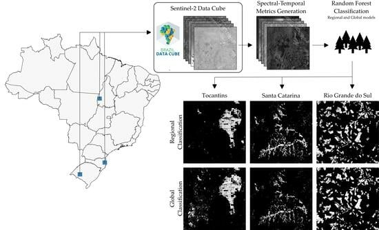
<p>Example of areas of training classified by the STM-based approach for the study regions compared to the official mapping for irrigated rice in Brazil. In black, the areas that are not rice are highlighted; in blue, areas of the ANA-CONAB mapping that were not classified by our approach are highlighted; in orange, areas classified as irrigated rice and not included in the official mapping are highlighted; in dark green, irrigated rice areas mapped by ANA-CONAB and our approach are highlighted. For Tocantins, the STM basic (<b>a</b>), STM Polar (<b>b</b>), STM Basic+Polar (<b>c</b>) and STM Global (<b>d</b>) classifications are shown. Similarly, Santa Catarina has STM basic (<b>e</b>), STM Polar (<b>f</b>), STM Basic+Polar (<b>g</b>) and STM Global (<b>h</b>) classifications. Finally, Rio Grande do Sul has classifications by STM basic (<b>i</b>), STM Polar (<b>j</b>), STM Basic+Polar (<b>k</b>) and STM Global (<b>l</b>) classifications.</p> ">
Figure 5
<p>Estimated rice-planted area for training region in Santa Catarina (<b>a</b>), Rio Grande do Sul (<b>b</b>) and Tocantins (<b>c</b>), and comparison between regional and global classifications and ANA-CONAB mapping.</p> ">
Figure 6
<p>Average confusion matrices for STM basic+polar classification in (<b>a</b>) Tocantins, (<b>b</b>) Santa Catarina, (<b>c</b>) Rio Grande do Sul, and (<b>d</b>) for global classification.</p> ">
Figure 7
<p>The most frequent important variables over the 100 iterations of the Monte Carlo simulation for the classification of basic+polar STMs classified by MeanDecreaseGini (<b>a</b>) and MeanDecreaseAccuracy (<b>b</b>).</p> ">
Figure 8
<p>Example of areas of validation classified by the STM-based approach for the study regions compared to the official mapping for irrigated rice in Brazil. In black, areas that are not rice are represented; in blue, areas of the ANA-CONAB mapping that were not classified by our approach are represented; in orange, areas classified as irrigated rice and not included in the official mapping are represented; in dark green, irrigated rice areas mapped by ANA-CONAB and our approach are represented. For Tocantins, the STM basic (<b>a</b>), STM Polar (<b>b</b>), STM Basic+Polar (<b>c</b>) and STM Global (<b>d</b>) classifications are shown. Similarly, Santa Catarina has STM basic (<b>e</b>), STM Polar (<b>f</b>), STM Basic+Polar (<b>g</b>) and STM Global (<b>h</b>) classifications. Finally, Rio Grande do Sul has classifications by STM basic (<b>i</b>), STM Polar (<b>j</b>), STM Basic+Polar (<b>k</b>) and STM Global (<b>l</b>) classifications.</p> ">
Figure 9
<p>Estimated rice-planted area for validation region in Santa Catarina (<b>a</b>), Rio Grande do Sul (<b>b</b>) and Tocantins (<b>c</b>), and comparison between regional and global classifications and ANA-CONAB mapping.</p> ">
Figure A1
<p>Validation pixel protocol for rice classes in Tocantins (validation samples #56 and #108). NDVI is light green, NDMI is dark green and NDWI is dark blue.</p> ">
Figure A2
<p>Validation pixel protocol for rice classes in Santa Catarina (validation samples #86 and #129). NDVI is light green, NDMI is dark green and NDWI is dark blue.</p> ">
Figure A3
<p>Validation pixel protocol for rice classes in Rio Grande do Sul (validation samples #56 and #120). NDVI is light green, NDMI is dark green and NDWI is dark blue.</p> ">
Review Reports Versions Notes

Abstract

:
Brazil, a leading rice producer globally, faces challenges in systematically mapping its diverse rice fields due to varying cropping systems, climates, and planting calendars. Existing rice mapping methods often rely on complex techniques like deep learning or microwave imagery, posing limitations for large-scale mapping. This study proposes a novel approach utilizing Sentinel-2 spectral–temporal metrics (STMs) in conjunction with a random forest classifier for rice paddy mapping. By extracting diverse STMs and training both regional and global classifiers, we validated the method across independent areas. While regional models tended to overestimate rice areas, the global model effectively reduced discrepancies between our data and the reference maps, achieving an overall classifier accuracy exceeding 80%. Despite the need for further refinement to address confusion with other crops, STM exhibits promise for national-scale rice paddy mapping in Brazil.

Graphical Abstract">

Graphical Abstract

1. Introduction

Rice stands as one of the most widely consumed foods globally, primarily cultivated under irrigation [1,2,3]. Understanding the spatial and temporal patterns of rice planting is paramount for effectively monitoring production, predicting harvests, managing stock, and regulating prices at both local and global scales [4,5,6]. Moreover, this knowledge directly aligns with the Sustainable Development Goals (SDGs), particularly those concerning food security.
Brazil is among the ten largest rice producers in the world, and its continental dimensions cover six biomes, five of which contribute to rice production: the Amazon, the Caatinga, the Cerrado, the Atlantic Forest, and the Pampas. Rice fields total more than 1,500,000 ha and are distributed in all regions of Brazil under tropical and subtropical climates. The most adopted cultivation system in rice production is irrigated [1,7,8,9]. The major rice contributor states in Brazil are Rio Grande do Sul, Santa Catarina, and e Tocantins, with its 2019–20 production being 9738.7 million tons [1,7].
Remote sensing (RS) data obtained from Earth observation (EO) satellites enable systematic analysis of the Earth’s surface and facilitate the monitoring and mapping of land use and land cover [5,10,11]. The use of RS data applied to agriculture allows the stage of crop development to be identified, estimating the harvest, mapping of crops, and crop intensity [12,13,14,15,16]. Although the use of RS data to map rice cultivation has been widely explored [1,17,18,19,20,21,22,23,24,25,26,27], the diverse growing seasons, cultivation practices, and spatial variability of rice cultivation still pose challenges for large-scale mapping [1,22,26,27].
Optical RS is the most used source of information for mapping rice paddies [22,26,27]. The possibility of investigating rice behavior at different wavelengths, as well as the use of spectral indices, allows for a variety of approaches to mapping rice. Time series analysis of spectral indices allows for the identification of key phenological characteristics, i.e., phenological algorithms, for rice classification, and this approach has proven accurate with different spatial-resolution sensors (30 m or more) [20,21,23,25]. However, phenological algorithms are based on the threshold approach, which is not easily transferable to different regions. Furthermore, optical data are susceptible to weather conditions, which affects the accuracy of time series-based approaches.
Recent advances in rice mapping have emphasized the utilization of microwave data, as they are less affected by rainfall interference in the microwave region. Additionally, the literature reflects a growing trend towards the use of deep learning algorithms for this purpose [17,18,26,28]. Nonetheless, the combined use of optical and microwave data produces more accurate classifications than the use of microwave data alone [28,29,30]. Furthermore, research indicates that the longer time series of optical data produces better classification results [31].
In this manner, Earth observations have been processed into analysis-ready data (ARD) and organized into data cubes, ensuring regular compositions in time and space, associated with a reference grid (tiles) processed at the surface reflectance level and such data cubes are accessible via cloud services, including Brazil Data Cube, SWISS Datacube, OpenEO, Australian Data Cube, Armenian Data Cube, Catalan Data Cube, and Africa Regional Data Cube [10,32,33,34,35,36,37]. ARDs facilitate the extraction of a consistent time series, which can then be employed in machine learning applications [10]. However, time series can be summarized in spectral–temporal metrics (STMs), which are statistical representations of time series that implicitly contain information about seasonal phenological variations in terrestrial targets [15,38,39,40,41,42,43]. Consequently, rice mapping methods based on the identification of key phenological periods can adopt STM, thereby overcoming the limitations of the threshold-based approach in terms of generalization. Moreover, the utilization of STM in LULC classifications is promising and has the potential to be applied on a national scale [15,40,41,44,45,46,47]. Nevertheless, the full potential of this approach for mapping irrigated rice has yet to be fully explored in Brazil.
In Brazil, recent initiatives have resulted in the production of national maps identifying rice paddy areas. The MapBiomas Brazil initiative mapped the rice crops of the main producing states, while the National Supply Company (CONAB), in partnership with the National Water Agency (ANA), carried out systematic mapping of irrigated rice in Brazil, with extensive fieldwork (2017–2020). Although previous work shows mappings based on C-band/Sentinel-1 microwave images and deep learning algorithms [17,18], a simple, robust, and automatic method to classify rice paddies over large areas is still needed.
Approaches combining the Synthetic Aperture Radar (SAR), particularly with C-band/Sentinel-1, and deep learning (DL) demand specialized knowledge and computational resources due to their inherent complexity [48]. DL methods require substantial data volumes and processing power, while fixed thresholds in vegetation indices lack adaptability to varying conditions. Moreover, existing methods often overlook the need to address large-scale regions, like those in Brazil, with diverse agricultural practices [17,18,48]. To address these limitations, our study proposes a straightforward approach utilizing spectral–temporal metrics from Sentinel-2 data alongside the random forest classifier for accurate rice paddy mapping. We evaluated this method in irrigated areas, specifically the National Irrigated Agriculture Poles (PNAIs), during the 2019/2020 crop year at a 10 m spatial resolution.

2. Materials and Methods

2.1. Study Region

The study area encompasses six regions, each covering approximately 11,151 km2, distributed across Tocantins (TO), Santa Catarina (SC), and Rio Grande do Sul (RS). Together, these states account for more than 90% of the area planted with rice in the country, or more than 1200 ha [1,7]. Each region intersects a National Pole of Irrigated Agriculture-Flooded Rice, which serves as a focal zone for irrigated production and holds potential for expansion in both area and water volume (see Figure 1) [49]. Rio Grande do Sul (946,000 ha), Santa Catarina (150,000 ha), and Tocantins (110,000 ha) are the three largest rice producers in Brazil, collectively dedicating over 1.2 million ha to rice cultivation [1,7].

2.1.1. Tocantins

PNAI Javaés-Formoso (tiles 026017 and 026018) lies within the equatorial region of Brazil and is part of the Cerrado biome. Classified as Aw according to the Köppen–Geiger system, this region denotes a savannah area with low/poorly distributed rainfall [50]. Rice planting in Tocantins is typically conducted between October and January, although a narrower window between October and November has been observed to reduce the climatic risks associated with planting [51,52,53]. This practice is already employed by producers. The average rice development cycle in the state is 150 days, with the harvest occurring between January and May [1,51,53,54].

2.1.2. Santa Catarina

PNAI Norte Catarinense (tiles 027033 and 027034) is situated in the subtropical region of Brazil and belongs to the Atlantic Forest biome. This region is classified as Cfa and Cfb, indicating regions without a dry season and characterized by hot, humid summers [50]. The planting period is between September and November, and the harvest takes place between January and April [1,51]. The rice development cycle is between 120 and 150 days [8,55]. The predominant cultivation system in the state is pre-germinated. In this system, the seeds are previously germinated, the planting area is planned, and a layer of water is maintained before transplanting, i.e., planting the pre-germinated seed [8,9,55].

2.1.3. Rio Grande do Sul

The Quaraí-Ibicuí-Icamaquã National Rice Production Area (tiles 020036 and 021037) is located on the Western Border of Rio Grande do Sul and is situated within the Pampa biome [8]. Planting takes place between September and December, with the harvesting period occurring between February and May [8,51]. The average development cycle of rice is 120 to 150 days [8].

2.2. Reference Data

The National Water and Sanitation Agency (ANA) and the National Supply Company (CONAB) have conducted the visual interpretation of Sentinel-2 imagery and field inspections to map irrigated rice in Brazil [1]. However, these mappings correspond to different crop years across the studied states (2017/2018 for TO; 2018/2019 for SC; 2019/2020 for RS). To harmonize the references, the 2019/2020 crop year was designated as the target year. The rice masks generated by ANA-CONAB were intersected with the rice mask provided by MapBiomas, which is based on convolutional neural networks and Landsat imagery [56]. The compatibility between the maps was made possible by the stability of the rice areas in Tocantins and Santa Catarina between 2019 and 2021 [57]. Furthermore, the results in the MapBiomas area were comparable to the reference data [56,57].
This intersection facilitated the sampling of rice points. This strategy was necessary to reduce the effort of sample collection and ensure representative samples of rice. Stratified samples for the non-rice class were generated using the MapBiomas 2020 land use and cover product, ensuring that the rice area was excluded to prevent confusion. The resulting samples underwent refinement through inspection by experts from INPE and ANA to eliminate spatial redundancy and retain representative samples.
The classification was validated using independent samples of both rice and non-rice areas collected from a different tile (refer to Table 1) to mitigate classification bias. These samples were gathered by analyzing the spectral–temporal behavior of the rice crop in each study area using the QGIS plugin GEE Timeseries Explorer [58] and inspecting the area with the color compositions B8A (R), B11 (G), and B12 (B) [1]. The protocol for visual interpretation to generate the samples, along with illustrated examples, is provided in Appendix A.

2.3. Remote Sensing Data

The Brazil Data Cube (BDC) is a project led by the National Institute for Space Research (INPE) with the goal of providing ready-to-use Earth observation data cubes [10]. The BDC offers a variety of data cubes from different sensors, such as MSI/Sentinel-2, OLI/Landsat-8, and WFI/CBERS-4. In this study, the Sentinel-2 (S2) data cube was selected, which contained data from 2019 to the present.
In the Sentinel-2 data cube, all spectral bands were resampled to a spatial resolution of 10 m and a temporal composition of 16 days. The compositions were made using the LCCF (Least Cloud-Cover First) method, which selects the most cloud-free pixels over a 16-day period [10].
In this study, informed by the literature review, three spectral indices were computed, including the Normalized Difference Moisture Index (NDMI) [59]; the Normalized Difference Vegetation Index (NDVI) [60]; and the Normalized Difference Water Index (NDWI) [61] (Equations (1)–(3)).
N D M I = ( N I R S W I R 1 ) ( N I R + S W I R 1 )
N D V I = ( N I R R e d ) ( N I R + R e d )
N D W I = ( G r e e n N I R ) ( G r e e n + N I R )

2.4. Time Series Extraction and STM Generation

The time series were generated for the three spectral indices from the rice samples for the period between 1 October 2019 and 1 October 2020, and the spectral–temporal behavior of the irrigated rice crops was investigated. This spectral–temporal profile enabled the identification of the crop and the determination of an optimal time window for the generation of spectral–temporal metrics (refer to Figure 2). After analyzing the planting calendar proposed by CONAB [51] and the agrometeorological zoning prepared by the Brazilian Agricultural Research Company (EMBRAPA) [62], as well as the spectral–temporal curves for each region, we selected the period between 1 October 2019 and 1 April 2020 as the time window for extracting the STM.
STMs can be divided into two groups: basic and polar [11]. The basic corresponds to descriptive statistics, while the polar corresponds to the representation of information in the polar plane and better represents cyclical processes [11,63,64]. The STMs were generated from the time series in the SITS package using the Sitsfeats package [64,65]. Table 2 shows the generated STMs and their corresponding descriptions adapted from [11,63]. The sets of STMs used are described in the next section.

2.5. Classification

The random forest (RF) algorithm was used for classification [66]. RF is a non-parametric machine learning algorithm based on decision trees. To mitigate errors inherent in individual trees, RF employs a collection of independently trained trees using random subsets of input data. The decision trees are trained using a random bag of sample attributes (bagging), and the class with the most votes among the trees is chosen to represent the sample (majority voting). Additionally, the algorithm’s implementation in R [67] allows variable importance using metrics like the Gini coefficient to be evaluated. The RF was built with 500 trees (ntree = 500), and the number of variables randomly sampled per split (mtry) was equal to the square root of the number of variables in the training set [68,69]. All steps were performed in R [67].
The attribute space for the classifications was divided into three input sets: basic STM, polar STM, and basic+polar STM. Basic STMs consist of the mean, mode, median, maximum, minimum, standard deviation, first quartile, second quartile, third quartile, interquartile range, and absolute mean derivative. The polar STMs correspond to the area per station (Q1, Q2, Q3, Q4), which divides the time series into quadrants, which are equispaced in time, eccentricity, and gyration radius. The basic and polar STMs are combined in the set of basic+polar STMs (see Table 2 for definitions). The global model, built with samples from all regions, used the basic+polar STM set.
The maps of the training areas were validated using Monte Carlo simulation with 100 iterations, in which, for each model, 70% of the samples for training and 30% for validation were randomly selected from the sample set [70,71]. For each iteration, the confusion matrix was calculated, and the average confusion matrix was used to derive the overall accuracy. The result of the best iteration was selected to generate the final maps of the training areas. The validation areas were classified as the best model from the training areas, and the average model was used to generate the binary confusion matrix (rice and non-rice) for these areas. To compare the municipal areas between each trained model, the classifications were polygonized, and polygons smaller than 1 ha were removed.

3. Results

3.1. Spectral–Temporal Profile for Rice

The time series of spectral indices covered the period between 1 October 2019 and 1 April 2020. Figure 2 shows the spectral–temporal behavior of irrigated rice in the study regions. It is important to note that the rice planting calendar and cultivation system in Brazil are not uniform [1,8]. In Santa Catarina, rice is mainly grown in a pregerminated system, where the crop is flooded before planting partially germinated grains [9], whereas in TO, direct seeding is used, and in RS, minimum tillage is used [1,8].
In Tocantins, two crop cycles were observed during the 2019/2020 harvest, with the first being rice. Between October and November, the NDVI curve exhibited values below 0.4, while the NDMI showed values below 0 and NDWI values above −0.4 (Figure 2a). This characterization corresponds to the presence of scrub vegetation or moist soil, indicative of the flooded phase of rice cultivation in Tocantins. In December, both NDVI and NDMI values increased, reaching their peak in February. However, between December and January, the NDVI curve exhibited a lower value, while the NDWI curve exhibited a higher value. This may be attributed to the cloud cover observed during the December images (3 December 2019, 45%; 19 December 2019, 37%). The Sentinel-2 data cube represents the pixels with the lowest cloud cover over the 16 days interval. Subsequently, in March, the NDVI and NDMI values declined while NDWI values increased, indicating the harvest of the initial crop. This harvest occurred after five months of cultivation or 150 days. The period of development required to cultivate rice cultivars utilized in Tocantins ranges from 120 to 160 days [53,54].
Santa Catarina (Figure 2b) exhibited an NDVI value exceeding 0.6 between October and December. The state employs a production system known as pregermination, involving flooding and maintaining a water layer on the crop, followed by the transplanting of germinated seeds [8]. The planting season in Santa Catarina typically begins in September, and the seeds are pre-germinated prior to transplantation. This practice may contribute to the higher NDVI value observed in this region compared to TO. In November, NDMI surpasses 0 and exceeds 0.2, while NDWI remains below −0.4 throughout the cycle until August 2020. Between November and December, a plateau in the NDVI and NDWI curves can be observed. The cloud cover over the rice samples ranged from 27% (1 November 2019) to 56% (17 November 2019), which may explain the plateau. The vegetative peak in Santa Catarina occurs between December and February, with harvest taking place between April and June.
In Rio Grande do Sul (Figure 2c), rice is planted between September and December, depending on the variety of cultivars used. Emergence occurs between October and November, with peak vegetation between January and March and harvest between April and May. The NDVI begins at 0.2 and increases in November, reaching its maximum value in February (~0.8). The estimated harvest period between April and May has an NDVI value of 0.2.

3.2. STM from Spectral Indices

The selection of NDMI, NDVI, and NDWI was based on their ability to identify different targets. NDMI is used to measure the water content in vegetation and utilizes bands in the mid-infrared (~1500–1800 nm) and near-infrared (~700–900 nm) bands. Other spectral indices used the same regions of the NDMI spectrum, such as NDWI [72], mNDVI [73], and LSWI [25]. LSWI is a popular index for irrigated rice mapping [26]. However, the spectral response returned was the same in all indices.
NDVI and NDWI are derived from the spectral responses of targets in the visible and near-infrared bands. NDVI emphasizes vegetation by contrasting the low reflectance in the visible (red band) with the higher reflectance in the near-infrared (NIR) band, which increases as vegetation matures. On the other hand, NDWI highlights water bodies by utilizing the NIR reflectance, which is minimal for water, in combination with green reflectance. NDVI is widely utilized in remote sensing due to its simplicity and effectiveness despite issues related to saturation caused by increased biomass. Meanwhile, NDWI facilitates the identification of water bodies, aiding in their differentiation from other terrestrial targets.
Therefore, spectral–temporal metrics (STMs) synthesize the behavior of time series spectral indices over a specified time window, which is essential for mapping irrigated rice (refer to Figure 3) [22,25,26,27]. The spectral–temporal behavior of each season is condensed into four quadrants, Q1-Q4 (Figure 3a–d), based on their respective STM areas. Q1 and Q4 highlight vegetation on riverbanks and cultivated areas, Q2 does not provide a significant highlight, and Q3 highlights wetlands or flooded areas. The gyration radius (refer to Figure 3f) highlights land use and land cover (LULC) classes with greater variability in temporal behavior or changes over time, which is particularly evident in agricultural land. The basic metrics describe the meaning of these features. The minimum (Figure 3h) STM reveals the lowest value of each pixel in the image. The standard deviation (Figure 3k) indicates changes over time, such as gyration radius. The interquartile range (Figure 3o) indicates the region where the pixel value increases over time. It is important to note that these metrics can highlight different aspects of the scene depending on the time window used.

3.3. Classification

The regional classifications, which utilized inputs such as basic, polar, and basic+polar STMs, are compared with the global classification, which relied on the basic+polar STM with respect to the official Brazilian mapping (ANA-CONAB) in Figure 4.
For Tocantins, the Javaés-Formoso Irrigation Project includes areas designated for rice cultivation, comprising systematized plots. Consequently, neighboring regions displaying similar flooding and maturation characteristics to other crops or types of vegetation were classified as irrigated rice. Although Figure 4a–d reveals ANA-CONAB mapping accurately delineating rice fields, the STM classification falls short of fully capturing these areas despite closely approaching this.
In Santa Catarina, the pre-germination system practiced in the state caused the classifier to erroneously map other land use and cover classes such as rice. The classification with polar STM showed the worst results visually. Figure 4f shows a river segment classified as rice. Looking at the global classification (Figure 4h), the commission on irrigated rice was reduced.
Despite yielding satisfactory results, the classification in Rio Grande do Sul was not entirely consistent with the ANA-CONAB map. Notably, the global classification misidentified many cultivated areas adjacent to rice plantations, which are likely irrigated or have a similar maturation cycle to rice. It is worth mentioning that rice cultivation in Rio Grande do Sul is interspersed with periods of soil rest (fallow), pasture, or rotation with other crops such as soybeans or maize. Given that the selected tiles did not encompass all municipalities within each state, municipal areas were compared with ANA-CONAB mapping (Figure 5). Subsequently, the average confusion matrices for Tocantins, Santa Catarina, Rio Grande do Sul, and the case of the Global model are depicted in Figure 6. It is important to note that only the basic+polar STM classification (both regional and global) was utilized to present the results in both cases.
For Santa Catarina (refer to Figure 5a), in comparison with the ANA-CONAB masks, the regional classification resulted in an overestimation of the rice-planted area in the municipality of Ilhota by 8%, Tijucas by 5%, and Itajaí by 31%, while underestimating the planted area in Gaspar by 15%. In the global classification, the area of Ilhota was overestimated by 1%; Tijucas was underestimated by 9%; Itajaí was overestimated by 27%; and Gaspar was underestimated by 10%. The performance of the global model effectively reduced uncertainty about the area estimate, bringing the mapped area of our classification closer to the official databases for Brazil.
In Rio Grande do Sul (Figure 5b), the area estimated by the regional classification was lower than the ANA-CONAB estimates in Cacequi (31% lower than the official area), Lavras do Sul (42%), Rosário do Sul (14%) and São Vicente (25%). In Sant’Ana do Livramento and São Gabriel, the percentage difference was close to 0. The omission of rice regions was due to confusion with other use classes, especially other types of agriculture. Rio Grande do Sul rotates the planting of rice with soybeans, corn, or fallow [1]. Furthermore, the rice planting period coincides with soybeans and corn. The development of crops under an irrigated regime can generate similar spectral curves over time, which may contribute to the omission of rice areas. In the global classification, the area of Cacequi was underestimated by 30%; Lavras do Sul by 29%; Rosário by 11%; São Vicente by 20%; Sant’Ana do Livramento by 2%; and in São Gabriel, there was an overestimate of 8%.
In Tocantins (Figure 5c), compared to the area computed in the ANA-CONAB mapping, the regional classification underestimated the areas of Lagoa da Confusão by 15% and Santa Rita do Tocantins by 46%. On the other hand, it overestimated the areas in Dueré by 2% and Formoso do Araguaia by 18%. In global classification, the overestimation of areas in Dueré and Formoso do Araguaia increased by 29% and 27%, respectively. In contrast, Santa Rita do Tocantins remained 46% underestimated, and Lagoa da Confusão reduced its underestimated area to 8%. These results show that the global model commissioned areas such as irrigated rice.
The confusion matrices indicate that the rice class was most frequently confused with the “agriculture” class. In all regions, there was corn or soybean planting, and crops whose planting and harvesting were within the time window were used [57]. Thus, it is possible that the “agriculture” class presented similar characteristics to the “rice” class, which caused the confusion. In Santa Catarina (refer to Figure 6b), commission errors occurred involving areas classified as agriculture, planted forest, and natural forest, along with omission errors with agriculture and natural forest. In Rio Grande do Sul (refer to Figure 6c), omission errors were observed with samples of agriculture, shrub vegetation, and water. The global matrix also highlights significant confusion with the agriculture class while also showing omission errors with pasture, natural forest, and shrub vegetation. Overall, the irrigated rice class was generally well classified, and the confusion with the agriculture class can be attributed to differences in the time window, which includes other summer cash crop cycles. Table 3 shows the binary confusion matrices used to assess the classification of rice in validation tiles.
The accuracy of the producer and the user are the measures that can be read from Table 3. Tocantins experienced the biggest omission out of all the classifications (user accuracy equaled 66%), with producer accuracy at more than 91%. The high omission that caused the Kappa index to be low was (0.65). Rio Grande do Sul had the highest overall accuracy (93%) and the best Kappa index (0.85). Santa Catarina had a good result, with user accuracy close to 90%, but producer accuracy was close to 80%. The global model showed great overall accuracy (~90%). This demonstrates that a global approach to classifying paddy fields in Brazil is possible, although the model needs to be improved. In all cases, it is hypothesized that the confusion between rice and non-rice is largely attributed to the “agriculture” class, as depicted in Figure 6. Figure 7 shows the ranking of the most frequent variables in global classification at the end of the 100 iterations of the Monte Carlo simulation.
Variable importance is a feature that facilitates the interpretability of classifiers. Two prominent importance measures are the mean decrease in impurity (MeanDecreaseGini) and permutation importance (MeanDecreaseAccuracy) [74]. However, Gini importance is not as reliable when the variables have disparate value scales, rendering the importance of permutation a more suitable option [75].
For this classification, the variables displayed comparable frequency for both measures of importance. The basic metrics based on the NDWI and NDVI indices were found to be the most relevant. Among these basic metrics, the NDVI_Q1 and NDWI_Q4 polar metrics were the only ones to emerge as the most important. Their significance is believed to stem from their association with the start and end of the crop cycle. Specifically, the NDWI_Q4 metric could be related to the presence of water at the beginning of the cycle, as highlighted by the NDWI, while the NDVI_Q1 metric captured biomass variation. Here, the Q1 metric corresponds to the first third of the time series, and the Q4 metric corresponds to the last third. Our time series covered six months (October to April). Thus, each Q metric concentrates information from about 45 days or three observations (16-day composites). Thus, Q1 concentrates information from the irrigation phase and rice flowering, while Q4 concentrates information from ripening and harvesting.
The classification of the validation areas is depicted in Figure 8. The classifications demonstrated good agreement with the ANA-CONAB map. However, classifications based solely on polar metrics exhibited the highest commission error, as they misclassified other land uses as rice, resulting in an overestimation of the area. Basic metrics were sensitive to other summer crops or wetlands in Tocantins. On the other hand, the classification using both basic and polar metrics showed more stable results, with reduced commission and omission areas. However, further refinements are still necessary.
Figure 9 shows the area planted with rice by the municipality in each validation region. The global model provided better area estimates in Tocantins (Figure 9a) and Rio Grande do Sul (Figure 9c). However, the state of Santa Catarina showed no gains with the global model (Figure 9b). The regional classifications underestimated the area planted in the municipalities, except in Santa Catarina, where three municipalities were overestimated.
In Tocantins, the classification assigned rice areas to the municipalities of Figueirópolis (~4 ha) and Sandolândia (~514 ha). The ANA-CONAB mapping did not include these municipalities, although the Instituto Brasileiro de Geografia e Estatística (IBGE) [57] showed that both municipalities had modest rice harvests (from 10 to 25 ha). In Rio Grande do Sul, there was confusion between agricultural areas and rice areas. The rice production in this state was diversified, being irrigated by flood irrigation and center pivot irrigation systems. In addition, other crops grown there also use irrigation, which can contribute to confusion between classes.

4. Discussion

This study investigated the results of classifications of rice fields in Brazil carried out by regional and global RF models based on spectral–temporal metrics. While previous studies have explored the combination of C-band/Sentinel-1 time series and deep learning, simpler methods using optical imaging time series have not been fully explored [17,18]. Our results are promising and suggest that spectral–temporal metrics derived from Sentinel-2 data cube spectral indices can be used to map rice fields. The suitability of this for the whole Brazilian territory needs to be demonstrated in future work.
The regional classifications demonstrated a high level of correlation with the official mapping, although they did present some limitations in differentiating irrigated rice from other types of land use, including other agricultural land uses (Figure 6). The states of Santa Catarina and Rio Grande do Sul exhibited the most favorable results. Tocantins, however, did not demonstrate the same degree of mapping accuracy (Table 3).
The global classification utilized a set of samples from all regions, affording the classifier the opportunity to assess the variability of rice cultivation in different conditions. Consequently, the classification for Tocantins exhibited more confusion between rice and other classes, specifically agriculture, water, and forests, whereas the Santa Catarina and Rio Grande do Sul classifications demonstrated a superior performance relative to the regional models (Figure 8). It is important to note that the quality of the training samples is crucial for the successful classification of irrigated rice. Our samples were based on official mapping carried out in the field by ANA and CONAB.
Spectral–temporal metrics are used for large-scale land use and land cover mapping, yielding positive outcomes, as evidenced by previous studies [40,41]. The flexibility in selecting the time window allows us to explore the specificities of terrestrial targets to optimize the classification. The incorporation of seasonality, which is inherent to STM, allows key phenological patterns of the rice crops to be obtained and compared to other LULC classes [15].
Frantz et al. described that annual STMs in tropical regions are somewhat inaccurate [43]. However, the availability of data improves the quality of the metrics. The data obtained from the Brazil Data Cube corresponds to images from 16 days, ensuring the availability of quality images throughout the study period. Moreover, central tendency metrics (e.g., mean, mode, median) are more consistent than variability metrics (e.g., standard deviation) and require fewer observations to be calculated reliably [43]. In this work, the central tendency metrics were more informative in the classifications, according to the importance measures (Figure 7). In this way, the dimensionality of the data itself could be reduced by focusing the classification on the use of STMs, such as the mean, median, minimum, and maximum [15].
Exploring other forms of data representation, such as Cartesian and polar planes, makes it possible to identify neglected cyclic patterns. In this study, it was observed that relying solely on the polar representation did not lead to noticeable improvements. The potential of using polar-based metrics can be explored to adapt to crop cycle shifts or by calculating the duration during which the accumulated vegetation index value, represented by the area, exceeds a certain threshold over a cycle period [76]. However, the combined use of basic and polar metrics showed promising potential in terms of complementarity.
Recent approaches tested for mapping rice in Brazil have predominantly focused on utilizing microwave remote sensing (C-band/Sentinel-1) and deep learning techniques [17,18]. While achieving accuracies higher than 95%, these studies primarily target specific test areas rather than nationwide coverage. However, the use of Sentinel-1 data poses challenges due to its high storage requirements, and processing these images can be time-consuming [17]. Although cloud solutions like Google Earth Engine ease accessibility and usage, strategies are necessary to optimize processing and prevent exceeding usage quotas. Additionally, employing deep learning for rice mapping is computationally intensive despite offering a high classification accuracy. Castro Filho et al. demonstrated comparable accuracies between the random forest algorithm and Long Short-Term Memory (LSTM) networks [18].
Pott et al. tested the combination of different data sources (MSI/Sentinel-2, C-band/Sentinel-1, and SRTM) [24]. The combined use of the three sources showed better results. It is recommended to utilize more accurate terrain models instead of SRTM as they better reflect the condition of the land [77]. Nonetheless, given the planned nature of rice cultivation areas, incorporating DEM as auxiliary data for classification may yield improved results [14,78].
The quality of training samples and the preprocessing of input data are crucial for achieving accurate results in rice classification [14,15,18,22,26,29,46]. Samples were sourced from validated field mapping by ANA and CONAB, alongside other partner organizations [1]. Processing involved the use of analysis-ready data from the Brazil Data Cube, consisting of temporal mosaics of Sentinel-2 data every 16 days, which was not found to be limiting for mapping. However, access to cloud-free images enhances the temporal composition, thereby improving the extraction of spectral–temporal metrics [39,40,41,42,43,79].

4.1. Relevant Contributions of This Study

Our work offers some insights into the mapping of rice paddies in Brazil. First, the importance of the variables allows new studies to use the attributes that are most appropriate to the purpose of the study for classification [15]. This allows the construction of a smaller attribute space; however, the accuracy of a rice field classification with fewer variables needs to be investigated.
We conducted an experiment and concluded that spectral–temporal metrics can be used to classify rice paddies with high accuracy, but our approach needs to be refined. The confusion with the agriculture class demonstrates that our approach needs to be refined to differentiate other summer crops, such as soybeans and corn, from rice fields (Figure 6). Other works use a lot of input data to extract spectral–temporal metrics, especially when it comes to crop-type mapping [15,44,45]. Longer optical time series produce more accurate classification results and provide more stable metrics [43,79,80]. Therefore, the STM allows the construction of a global model for mapping rice paddies [15,46]. This is the most relevant contribution of this article, as it can simplify the process of systematic mapping in rice paddies and can perhaps be transferred to other crops. Furthermore, our approach demonstrated efficacy with a representative sample set. The collection of samples in the field is costly, and the availability of very high spatial-resolution images may not keep pace with the dynamics of land use. Medium spatial-resolution images can lead to interpretation errors in complex agricultural landscapes. Therefore, a representative set of samples associated with a transferable model in time is the most suitable.

4.2. Limitations and Future Works

Despite promising results, some challenges remain. First, the transferability of the models over time was not tested. We only benefited from one crop year, and knowing whether the model was applicable in other years favored our objective of developing a simple and scalable method. Pham et al. demonstrated that the transferability of an STM-based model is dependent upon the availability of Clear-Sky Observations in the training year and the application years [79]. Our approach employed time-regular compositions, as it utilized data cubes, which may enhance the transferability of models over time.
The impact of the time window on the classification results was also not investigated. We selected an optimal period and used it in the work. However, polar analyses did not benefit from such a restricted time frame. The basic specifications, in turn, tend to produce better results the longer the time window, depending on the availability of quality data. Other works have invested in annual or interannual time windows to extract reliable STMs [15,43,44,46,80].
Auxiliary data were not included in this work. Information from Digital Elevation Models can assist in the rice field mapping process, depending on the specificity of the crop [14,80]. Furthermore, climate data can improve separability between agriculture and other classes. Paddy field mapping must be capable of differentiating other agricultural crops. Our study did not segregate specific data sets for maize and soybeans, and our approach must be validated on a sample set that includes these classes to verify the method’s efficacy in separating these crops. The utilization of STM extracted from reflectance bands or spectral indices in agricultural-type classification yielded favorable outcomes in several regions. However, a larger attribute space was utilized in each case [15,44,45,46,78].
Finally, Brazil’s classification at a national level was the goal of this initiative. Therefore, the expansion of study areas is the subject of future work.

5. Conclusions

In this study, we proposed an approach based on spectral–temporal metrics derived from Sentinel-2 analysis-ready data time series to map paddy fields in different regions of Brazil and evaluated the potential for classification generalization over different spatial extents. The analysis of the time series of spectral indices of irrigated rice made it possible to identify an optimum time window between October and April that is common to all the study regions for the extraction of STM. Other studies based on the time series of optical data, such as phenological algorithms, encounter difficulties in transferring their approaches to new areas. Our approach addresses this challenge by employing spectral–temporal metrics derived from spectral indices in an optimal time window. Our main findings are as follows: (i) our results indicate that a global classification is feasible for Brazil; (ii) regional models encounter challenges in a specific crop system (pre-germinated); (iii) the most important variables are basic metrics; and (iv) the most frequent and important variables are related to NDMI. Therefore, the use of STMs to classify irrigated rice in Brazil is recommended and has the potential to provide classification at a national level. For future work, it is necessary to expand the mapping area in order to address the complexity of land uses and land cover, including a variety of crops. In addition, it is essential to verify the transferability of the model over time and to investigate the impact of the sample set size.

Author Contributions

Conceptualization, L.M.G.F. and H.d.N.B.; methodology, L.M.G.F., H.d.N.B. and A.S.F.F.; software, A.S.F.F. and H.d.N.B.; validation, A.S.F.F. and H.d.N.B.; formal analysis, A.S.F.F., L.M.G.F. and H.d.N.B.; investigation, A.S.F.F.; resources, L.M.G.F.; writing—original draft preparation, A.S.F.F.; writing—review and editing, H.d.N.B. and L.M.G.F.; supervision, L.M.G.F. and H.d.N.B.; project administration, L.M.G.F.; funding acquisition, L.M.G.F. All authors have read and agreed to the published version of the manuscript.

Funding

This study was financed in part by the “Coordenação de Aperfeiçoamento de Pessoal de Nível Superior (CAPES)”—Finance Code 001.

Data Availability Statement

The original contributions presented in the study are included in the article, further inquiries can be directed to the corresponding author.

Acknowledgments

The authors would like to thank CNPq (Process 423959/2021-2) and Brazil Data Cube (a project that is part of the “Environmental Monitoring of Brazilian Biomes”, financed by the Amazon Fund through the financial collaboration of the National Bank for Economic and Social Development (BNDES) and the Foundation for Science, Technology and Space Applications (FUNCATE) no. 17.2.0536.1) for the availability of free and open source software that was useful for this research.

Conflicts of Interest

The authors declare no conflicts of interest.

Appendix A

Figure A1. Validation pixel protocol for rice classes in Tocantins (validation samples #56 and #108). NDVI is light green, NDMI is dark green and NDWI is dark blue.
Remotesensing 16 02900 g0a1
Figure A2. Validation pixel protocol for rice classes in Santa Catarina (validation samples #86 and #129). NDVI is light green, NDMI is dark green and NDWI is dark blue.
Remotesensing 16 02900 g0a2
Figure A3. Validation pixel protocol for rice classes in Rio Grande do Sul (validation samples #56 and #120). NDVI is light green, NDMI is dark green and NDWI is dark blue.
Remotesensing 16 02900 g0a3

References

  1. Agência Nacional de Águas e Saneamento Básico (ANA). Mapeamento Do Arroz Irrigado No Brasil; ANA: Brasília, Brazil, 2020. [Google Scholar]
  2. Rodrigues, R.M.; Souza, A.D.M.; Bezerra, I.N.; Pereira, R.A.; Yokoo, E.M.; Sichieri, R. Most Consumed Foods in Brazil: Evolution between 2008–2009 and 2017–2018. Rev. Saude Publica 2021, 55, 4s. [Google Scholar] [CrossRef] [PubMed]
  3. Sociedade Sul-Brasileira de Arroz Irrigado. Arroz Irrigado: Recomendações Técnicas Da Pesquisa Para o Sul Do Brasil; Sociedade Sul-Brasileira de Arroz Irrigado: Cachoeirinha, Brazil, 2018; ISBN 978-85-54856-29-8. [Google Scholar]
  4. Laborte, A.G.; Gutierrez, M.A.; Balanza, J.G.; Saito, K.; Zwart, S.J.; Boschetti, M.; Murty, M.V.R.; Villano, L.; Aunario, J.K.; Reinke, R.; et al. RiceAtlas, a Spatial Database of Global Rice Calendars and Production. Sci. Data 2017, 4, 170074. [Google Scholar] [CrossRef] [PubMed]
  5. Bendini, H.N.; Garcia Fonseca, L.M.; Schwieder, M.; Sehn Körting, T.; Rufin, P.; Del Arco Sanches, I.; Leitão, P.J.; Hostert, P. Detailed Agricultural Land Classification in the Brazilian Cerrado Based on Phenological Information from Dense Satellite Image Time Series. Int. J. Appl. Earth Obs. Geoinf. 2019, 82, 101872. [Google Scholar] [CrossRef]
  6. Formaggio, A.R.; Sanches, I.D. Sensoriamento Remoto em Agricultura; Oficina de Textos: São Paulo, Brazil, 2017; ISBN 978-85-7975-282-7. [Google Scholar]
  7. Companhia Nacional de Abastecimento (CONAB). Série Histórica Da Safra de Arroz 2023. Available online: https://www.conab.gov.br/info-agro/safras/serie-historica-das-safras/itemlist/category/900-arroz (accessed on 14 August 2023).
  8. de Magalhães, A.M., Jr.; Gomes, A.D.S.; dos Santos, A.B. Sistema de Cultivo de Arroz Irrigado No Brasil; Sistemas de Produção; Embrapa Clima Temperado: Pelotas, Brazil, 2004; p. 270. [Google Scholar]
  9. EMBRAPA, Empresa Brasileira de Pesquisa Agropecuária. Cultivo Do Arroz. Available online: https://www.embrapa.br/en/agencia-de-informacao-tecnologica/cultivos/arroz (accessed on 16 October 2023).
  10. Ferreira, K.R.; Queiroz, G.R.; Vinhas, L.; Marujo, R.F.B.; Simões, R.E.O.; Picoli, M.C.A.; Camara, G.; Cartaxo, R.; Gomes, V.C.F.; Santos, L.A.; et al. Earth Observation Data Cubes for Brazil: Requirements, Methodology and Products. Remote Sens. 2020, 12, 4033. [Google Scholar] [CrossRef]
  11. Körting, T.S.; Garcia Fonseca, L.M.; Câmara, G. GeoDMA-Geographic Data Mining Analyst. Comput. Geosci. 2013, 57, 133–145. [Google Scholar] [CrossRef]
  12. He, Y.; Dong, J.; Liao, X.; Sun, L.; Wang, Z.; You, N.; Li, Z.; Fu, P. Examining Rice Distribution and Cropping Intensity in a Mixed Single- and Double-Cropping Region in South China Using All Available Sentinel 1/2 Images. Int. J. Appl. Earth Obs. Geoinf. 2021, 101, 102351. [Google Scholar] [CrossRef]
  13. He, Z.; Li, S.; Chang, M.; Liu, Y.; Liu, K.; Wan, L.; Wang, Y. Novel Harmonic-Based Scheme for Mapping Rice-Crop Intensity at a Large Scale Using Time-Series Sentinel-1 and ERA5-Land Datasets. IEEE Trans. Geosci. Remote Sens. 2024, 62, 1–23. [Google Scholar] [CrossRef]
  14. Som-ard, J.; Immitzer, M.; Vuolo, F.; Ninsawat, S.; Atzberger, C. Mapping of Crop Types in 1989, 1999, 2009 and 2019 to Assess Major Land Cover Trends of the Udon Thani Province, Thailand. Comput. Electron. Agric. 2022, 198, 107083. [Google Scholar] [CrossRef]
  15. You, N.; Dong, J.; Huang, J.; Du, G.; Zhang, G.; He, Y.; Yang, T.; Di, Y.; Xiao, X. The 10-m Crop Type Maps in Northeast China during 2017–2019. Sci. Data 2021, 8, 41. [Google Scholar] [CrossRef]
  16. Karthikeyan, L.; Chawla, I.; Mishra, A.K. A Review of Remote Sensing Applications in Agriculture for Food Security: Crop Growth and Yield, Irrigation, and Crop Losses. J. Hydrol. 2020, 586, 124905. [Google Scholar] [CrossRef]
  17. Bem, P.P.; de Carvalho Júnior, O.A.; de Carvalho, O.L.F.; Gomes, R.A.T.; Guimarāes, R.F.; Pimentel, C.M.M. Irrigated Rice Crop Identification in Southern Brazil Using Convolutional Neural Networks and Sentinel-1 Time Series. Remote Sens. Appl. Soc. Environ. 2021, 24, 100627. [Google Scholar] [CrossRef]
  18. de Castro Filho, H.C.; de Carvalho, O.A., Jr.; de Carvalho, O.L.F.; de Bem, P.P.; de Moura, R.D.S.; de Albuquerque, A.O.; Silva, c.R.; Guimaraes Ferreira, P.H.; Guimaraes, R.F.; Trancoso Gomes, R.A. Rice Crop Detection Using LSTM, Bi-LSTM, and Machine Learning Models from Sentinel-1 Time Series. Remote Sens. 2020, 12, 2655. [Google Scholar] [CrossRef]
  19. D’Arco, E.; Alvarenga, B.S.; Rizzi, R.; Rudorff, B.F.T.; Moreira, M.A.; Adami, M. Geotecnologias na Estimativa da Área Plantada Com Arroz Irrigado. Rev. Bras. Cartogr. 2009, 58, 247–253. [Google Scholar] [CrossRef]
  20. Dong, J.; Xiao, X.; Kou, W.; Qin, Y.; Zhang, G.; Li, L.; Jin, C.; Zhou, Y.; Wang, J.; Biradar, C.; et al. Tracking the Dynamics of Paddy Rice Planting Area in 1986–2010 through Time Series Landsat Images and Phenology-Based Algorithms. Remote Sens. Environ. 2015, 160, 99–113. [Google Scholar] [CrossRef]
  21. Dong, J.; Xiao, X.; Menarguez, M.A.; Zhang, G.; Qin, Y.; Thau, D.; Biradar, C.; Moore, B. Mapping Paddy Rice Planting Area in Northeastern Asia with Landsat 8 Images, Phenology-Based Algorithm and Google Earth Engine. Remote Sens. Environ. 2016, 185, 142–154. [Google Scholar] [CrossRef] [PubMed]
  22. Dong, J.; Xiao, X. Evolution of Regional to Global Paddy Rice Mapping Methods: A Review. ISPRS J. Photogramm. Remote Sens. 2016, 119, 214–227. [Google Scholar] [CrossRef]
  23. Kontgis, C.; Schneider, A.; Ozdogan, M. Mapping Rice Paddy Extent and Intensification in the Vietnamese Mekong River Delta with Dense Time Stacks of Landsat Data. Remote Sens. Environ. 2015, 169, 255–269. [Google Scholar] [CrossRef]
  24. Pott, L.P.; Amado, T.J.C.; Schwalbert, R.A.; Corassa, G.M.; Ciampitti, I.A. Satellite-Based Data Fusion Crop Type Classification and Mapping in Rio Grande Do Sul, Brazil. ISPRS J. Photogramm. Remote Sens. 2021, 176, 196–210. [Google Scholar] [CrossRef]
  25. Xiao, X.; Hollinger, D.; Aber, J.; Goltz, M.; Davidson, E.A.; Zhang, Q.; Moore, B. Satellite-Based Modeling of Gross Primary Production in an Evergreen Needleleaf Forest. Remote Sens. Environ. 2004, 89, 519–534. [Google Scholar] [CrossRef]
  26. Zhao, R.; Li, Y.; Ma, M. Mapping Paddy Rice with Satellite Remote Sensing: A Review. Sustainability 2021, 13, 503. [Google Scholar] [CrossRef]
  27. Kuenzer, C.; Knauer, K. Remote Sensing of Rice Crop Areas. Int. J. Remote Sens. 2013, 34, 2101–2139. [Google Scholar] [CrossRef]
  28. Saini, P.; Nagpal, B. Spatiotemporal Landsat-Sentinel-2 Satellite Imagery-Based Hybrid Deep Neural Network for Paddy Crop Prediction Using Google Earth Engine. Adv. Space Res. 2024, 73, 4988–5004. [Google Scholar] [CrossRef]
  29. Sun, L.; Yang, T.; Lou, Y.; Shi, Q.; Zhang, L. Paddy Rice Mapping Based on Phenology Matching and Cultivation Pattern Analysis Combining Multi-Source Data in Guangdong, China. J. Remote Sens. 2024, 0152. [Google Scholar] [CrossRef]
  30. Qiu, B.; Yu, L.; Yang, P.; Wu, W.; Chen, J.; Zhu, X.; Duan, M. Mapping Upland Crop–Rice Cropping Systems for Targeted Sustainable Intensification in South China. Crop J. 2024, 12, 614–629. [Google Scholar] [CrossRef]
  31. Ofori-Ampofo, S.; Pelletier, C.; Lang, S. Crop Type Mapping from Optical and Radar Time Series Using Attention-Based Deep Learning. Remote Sens. 2021, 13, 4668. [Google Scholar] [CrossRef]
  32. Appel, M.; Pebesma, E. On-Demand Processing of Data Cubes from Satellite Image Collections with the Gdalcubes Library. Data 2019, 4, 92. [Google Scholar] [CrossRef]
  33. Lewis, A.; Oliver, S.; Lymburner, L.; Evans, B.; Wyborn, L.; Mueller, N.; Raevksi, G.; Hooke, J.; Woodcock, R.; Sixsmith, J.; et al. The Australian Geoscience Data Cube—Foundations and Lessons Learned. Remote Sens. Environ. 2017, 202, 276–292. [Google Scholar] [CrossRef]
  34. Giuliani, G.; Chatenoux, B.; De Bono, A.; Rodila, D.; Richard, J.P.; Allenbach, K.; Dao, H.; Peduzzi, P. Building an Earth Observations Data Cube: Lessons Learned from the Swiss Data Cube (SDC) on Generating Analysis Ready Data (ARD). Big Earth Data 2017, 1, 100–117. [Google Scholar] [CrossRef]
  35. Asmaryan, S.; Muradyan, V.; Tepanosyan, G.; Hovsepyan, A.; Saghatelyan, A.; Astsatryan, H.; Grigoryan, H.; Abrahamyan, R.; Guigoz, Y.; Giuliani, G. Paving the Way towards an Armenian Data Cube. Data 2019, 4, 117. [Google Scholar] [CrossRef]
  36. Maso, J.; Zabala, A.; Serral, I.; Pons, X. A Portal Offering Standard Visualization and Analysis on Top of an Open Data Cube for Sub-National Regions: The Catalan Data Cube Example. Data 2019, 4, 96. [Google Scholar] [CrossRef]
  37. Killough, B. The Impact of Analysis Ready Data in the Africa Regional Data Cube. In Proceedings of the IGARSS 2019—2019 IEEE International Geoscience and Remote Sensing Symposium, Yokohama, Japan, 28 July–2 August 2019; IEEE: Piscataway, NJ, USA, 2019; pp. 5646–5649. [Google Scholar]
  38. Rufin, P.; Müller, D.; Schwieder, M.; Pflugmacher, D.; Hostert, P. Landsat Time Series Reveal Simultaneous Expansion and Intensification of Irrigated Dry Season Cropping in Southeastern Turkey. J. Land Use Sci. 2021, 16, 94–110. [Google Scholar] [CrossRef]
  39. Schug, F.; Frantz, D.; Okujeni, A.; Van Der Linden, S.; Hostert, P. Mapping Urban-Rural Gradients of Settlements and Vegetation at National Scale Using Sentinel-2 Spectral-Temporal Metrics and Regression-Based Unmixing with Synthetic Training Data. Remote Sens. Environ. 2020, 246, 111810. [Google Scholar] [CrossRef] [PubMed]
  40. Griffiths, P.; Van Der Linden, S.; Kuemmerle, T.; Hostert, P. A Pixel-Based Landsat Compositing Algorithm forLarge Area Land Cover Mapping. IEEE J. Sel. Top. Appl. Earth Obs. Remote Sens. 2013, 6, 2088–2101. [Google Scholar] [CrossRef]
  41. Griffiths, P.; Nendel, C.; Hostert, P. Intra-Annual Reflectance Composites from Sentinel-2 and Landsat for National-Scale Crop and Land Cover Mapping. Remote Sens. Environ. 2019, 220, 135–151. [Google Scholar] [CrossRef]
  42. Pflugmacher, D.; Rabe, A.; Peters, M.; Hostert, P. Mapping Pan-European Land Cover Using Landsat Spectral-Temporal Metrics and the European LUCAS Survey. Remote Sens. Environ. 2019, 221, 583–595. [Google Scholar] [CrossRef]
  43. Frantz, D.; Rufin, P.; Janz, A.; Ernst, S.; Pflugmacher, D.; Schug, F.; Hostert, P. Understanding the Robustness of Spectral-Temporal Metrics across the Global Landsat Archive from 1984 to 2019—A Quantitative Evaluation. Remote Sens. Environ. 2023, 298, 113823. [Google Scholar] [CrossRef]
  44. Bendini, H.N.; Fonseca, L.M.G.; Bertolini, C.A.; Mariano, R.F.; Fernandes Filho, A.S.; Fontenelle, T.H.; Ferreira, D.A.C. Irrigated Agriculture Mapping in a Semi-Arid Region in Brazil Based on the Use of Sentinel-2 Data and Random Forest Algorithm. Int. Arch. Photogramm. Remote Sens. Spat. Inf. Sci. 2023, 48, 33–39. [Google Scholar] [CrossRef]
  45. Ibrahim, E.S.; Rufin, P.; Nill, L.; Kamali, B.; Nendel, C.; Hostert, P. Mapping Crop Types and Cropping Systems in Nigeria with Sentinel-2 Imagery. Remote Sens. 2021, 13, 3523. [Google Scholar] [CrossRef]
  46. Xuan, F.; Dong, Y.; Li, J.; Li, X.; Su, W.; Huang, X.; Huang, J.; Xie, Z.; Li, Z.; Liu, H.; et al. Mapping Crop Type in Northeast China during 2013–2021 Using Automatic Sampling and Tile-Based Image Classification. Int. J. Appl. Earth Obs. Geoinf. 2023, 117, 103178. [Google Scholar] [CrossRef]
  47. Yin, H.; Brandão, A.; Buchner, J.; Helmers, D.; Iuliano, B.G.; Kimambo, N.E.; Lewińska, K.E.; Razenkova, E.; Rizayeva, A.; Rogova, N.; et al. Monitoring Cropland Abandonment with Landsat Time Series. Remote Sens. Environ. 2020, 246, 111873. [Google Scholar] [CrossRef]
  48. Xia, L.; Zhao, F.; Chen, J.; Yu, L.; Lu, M.; Yu, Q.; Liang, S.; Fan, L.; Sun, X.; Wu, S.; et al. A Full Resolution Deep Learning Network for Paddy Rice Mapping Using Landsat Data. ISPRS J. Photogramm. Remote Sens. 2022, 194, 91–107. [Google Scholar] [CrossRef]
  49. Agência Nacional de Águas e Saneamento Básico (ANA). Polos Nacionais de Agricultura Irrigada; ANA: Brasília, Brazil, 2020. [Google Scholar]
  50. Beck, H.E.; Zimmermann, N.E.; McVicar, T.R.; Vergopolan, N.; Berg, A.; Wood, E.F. Present and Future Köppen-Geiger Climate Classification Maps at 1-Km Resolution. Sci. Data 2018, 5, 180214. [Google Scholar] [CrossRef] [PubMed]
  51. Companhia Nacional de Abastecimento (CONAB). Calendário de Plantio e Colheita de Grãos No Brasil 2020. Available online: https://www.conab.gov.br/institucional/publicacoes/outras-publicacoes/item/15406-calendario-agricola-plantio-e-colheita?platform=hootsuite (accessed on 27 July 2023).
  52. Fragoso, D.D.B.; Alves, E.; Expedito, C.; Cardoso, A.; Rodrigues De Souza, C.E.; Rodrigues De Souza, E.; Ferreira, C.M. Caracterização e Diagnóstico Da Cadeia Produtiva Do Arroz No Estado Do Tocantins; Embrapa: Brasília, Distrito Federal, 2013; ISBN 978-85-7035-226-2. [Google Scholar]
  53. Fragoso, D.D.B.; Hideo Nakano Rangel, P.; Carvalho da Rocha, R.N.; Alves Cardoso, E. Contribuição Das Cultivares de Arroz Da Embrapa NA Produção de Arroz Irrigado No Estado Do Tocantins. Agri-Environ. Sci. 2021, 7, 6. [Google Scholar] [CrossRef]
  54. dos Santos, A.B.; Santiago, C.M. Informações Técnicas Para a Cultura Do Arroz Irrigado Nas Regiões Norte e Nordeste Do Brasil; Embrapa: Brasília, Brazil, 2014. [Google Scholar]
  55. Lima Campos, M.; Rodrigues, V.E.; Organizadores, H. Recomendações Para a Produção Sustentável de Arroz Irrigado Em Santa Catarina: 4ª. edição. Sist. Produção 2022, 56. Available online: https://publicacoes.epagri.sc.gov.br/SP/article/view/1587 (accessed on 19 June 2024).
  56. MapBiomas. MapBiomas Irrigation-Appendix. Available online: https://brasil.mapbiomas.org/download-dos-atbds-com-metodo-detalhado/ (accessed on 10 April 2023).
  57. Instituto Brasileiro de Geografia e Estatística (IBGE). Produção Agrícola Municipal 2023: Tabela 1612—Área Plantada, Área Colhida, Quantidade Produzida, Rendimento Médio e Valor Da Produção Das Lavouras Temporárias. Available online: https://sidra.ibge.gov.br/tabela/1612 (accessed on 8 January 2024).
  58. Rufin, P.; Rabe, A.; Nill, L.; Hostert, P. Gee Timeseries Explorer for Qgis—Instant Access to Petabytes of Earth Observation Data. Int. Arch. Photogramm. Remote Sens. Spat. Inf. Sci. 2021, 46, 155–158. [Google Scholar] [CrossRef]
  59. Hardisky, M.A.; Klemas, V.; Smart, R.M. The Influence of Soil Salinity, Growth Form, and Leaf Moisture on-the Spectral Radiance of Spartina Alterniflora Canopies. Photogramm. Eng. Remote Sens. 1983, 49, 77–83. [Google Scholar]
  60. Rouse, J.W., Jr.; Haas, R.H.; Schell, J.A.; Deering, D.W. Monitoring Vegetation Systems in the Great Plains with ERTS. In Proceedings of the Third Earth Resources Technology Satellite-1 Symposium, Goddard Space Flight Center, Washington, DC, USA, 10–14 December 1973; pp. 309–317. [Google Scholar]
  61. McFeeters, S.K. The Use of the Normalized Difference Water Index (NDWI) in the Delineation of Open Water Features. Int. J. Remote Sens. 1996, 17, 1425–1432. [Google Scholar] [CrossRef]
  62. Ministério da Agricultura e Pecuária (MAPA). Painel de Indicação de Riscos. Available online: https://mapa-indicadores.agricultura.gov.br/publico/extensions/Zarc/Zarc.html (accessed on 22 January 2024).
  63. Soares, A.R.; Bendini, H.N.; Vaz, D.V.; Uehara, T.D.T.; Neves, A.K.; Lechler, S.; Körting, T.S.; G Fonseca, L.M. Stmetrics: A Python Package for Satellite Image Time-Series Feature Extraction. In Proceedings of the IGARSS 2020—2020 IEEE International Geoscience and Remote Sensing Symposium, Waikoloa, HI, USA, 26 September–2 October 2020. [Google Scholar]
  64. Carvalho, F. Sitsfeats 2021. Available online: https://rdrr.io/cran/sitsfeats/ (accessed on 18 December 2023).
  65. Simões, R.; Camara, G.; Queiroz, G.; Souza, F.; Andrade, P.R.; Santos, L.; Carvalho, A.; Ferreira, K. Satellite Image Time Series Analysis for Big Earth Observation Data. Remote Sens. 2021, 13, 2428. [Google Scholar] [CrossRef]
  66. Breiman, L. Random Forests. Mach. Learn. 2001, 45, 5–32. [Google Scholar] [CrossRef]
  67. R Core Team. R Language Definition; R Foundation for Statistical Computing: Vienna, Austria, 2022. [Google Scholar]
  68. Belgiu, M.; Drăguţ, L. Random Forest in Remote Sensing: A Review of Applications and Future Directions. ISPRS J. Photogramm. Remote Sens. 2016, 114, 24–31. [Google Scholar] [CrossRef]
  69. Maxwell, A.E.; Warner, T.A.; Fang, F. Implementation of Machine-Learning Classification in Remote Sensing: An Applied Review. Int. J. Remote Sens. 2018, 39, 2784–2817. [Google Scholar] [CrossRef]
  70. Jiang, X.; Fang, S.; Huang, X.; Liu, Y.; Guo, L. Rice Mapping and Growth Monitoring Based on Time Series GF-6 Images and Red-Edge Bands. Remote Sens. 2021, 13, 579. [Google Scholar] [CrossRef]
  71. Rubinstein, R.Y.; Kroese, D.P. Simulation and the Monte Carlo Method, 1st ed.; Wiley Series in Probability and Statistics; Wiley: Hoboken, NJ, USA, 2016; ISBN 978-1-118-63216-1. [Google Scholar]
  72. Gao, B. NDWI—A Normalized Difference Water Index for Remote Sensing of Vegetation Liquid Water from Space. Remote Sens. Environ. 1996, 58, 257–266. [Google Scholar] [CrossRef]
  73. Jurgens, C. The Modified Normalized Difference Vegetation Index (mNDVI) a New Index to Determine Frost Damages in Agriculture Based on Landsat TM Data. Int. J. Remote Sens. 1997, 18, 3583–3594. [Google Scholar] [CrossRef]
  74. Parr, T.; Turgutlu, K.; Csiszar, C.; Howard, J. Beware Default Random Forest Importances. Available online: https://explained.ai/rf-importance/ (accessed on 28 December 2023).
  75. Strobl, C.; Boulesteix, A.-L.; Zeileis, A.; Hothorn, T. Bias in Random Forest Variable Importance Measures: Illustrations, Sources and a Solution. BMC Bioinform. 2007, 8, 25. [Google Scholar] [CrossRef] [PubMed]
  76. Brooks, B.-G.J.; Lee, D.C.; Pomara, L.Y.; Hargrove, W.W. Monitoring Broadscale Vegetational Diversity and Change across North American Landscapes Using Land Surface Phenology. Forests 2020, 11, 606. [Google Scholar] [CrossRef]
  77. Bielski, C.; López-Vázquez, C.; Grohmann, C.H.; Guth, P.L.; Hawker, L.; Gesch, D.; Trevisani, S.; Herrera-Cruz, V.; Riazanoff, S.; Corseaux, A.; et al. Novel Approach for Ranking DEMs: Copernicus DEM Improves One Arc Second Open Global Topography. IEEE Trans. Geosci. Remote Sens. 2024, 62, 1–22. [Google Scholar] [CrossRef]
  78. Suwanlee, S.R.; Keawsomsee, S.; Pengjunsang, M.; Homtong, N.; Prakobya, A.; Borgogno-Mondino, E.; Sarvia, F.; Som-ard, J. Monitoring Agricultural Land and Land Cover Change from 2001–2021 of the Chi River Basin, Thailand Using Multi-Temporal Landsat Data Based on Google Earth Engine. Remote Sens. 2023, 15, 4339. [Google Scholar] [CrossRef]
  79. Pham, V.-D.; Thiel, F.; Frantz, D.; Okujeni, A.; Schug, F.; van der Linden, S. Learning the Variations in Annual Spectral-Temporal Metrics to Enhance the Transferability of Regression Models for Land Cover Fraction Monitoring. Remote Sens. Environ. 2024, 308, 114206. [Google Scholar] [CrossRef]
  80. Wohlfart, C.; Mack, B.; Liu, G.; Kuenzer, C. Multi-Faceted Land Cover and Land Use Change Analyses in the Yellow River Basin Based on Dense Landsat Time Series: Exemplary Analysis in Mining, Agriculture, Forest, and Urban Areas. Appl. Geogr. 2017, 85, 73–88. [Google Scholar] [CrossRef]
Figure 1. Study region and validation sampling distribution. Two tiles (training and validation) were selected for each National Pole of Irrigated Agriculture. Black points represent non-rice samples, while green points represent rice samples.
Remotesensing 16 02900 g001
Figure 2. Rice spectral–temporal profile for each study region in Tocantins (a), Santa Catarina (b), and Rio Grande do Sul (c). The spectral indices are NDVI (green), NDMI (orange), and NDWI (blue).
Remotesensing 16 02900 g002
Figure 3. An example of spectral–temporal metrics (STM) for Rio Grande do Sul (RS). The red line is the contour of the rice mapping by ANA-CONAB (2019/2020). The polar metrics Q1 (a), Q2 (b), Q3 (c), Q4 (d), and Eccentricity (e) provide less contrast. On the other hand, Gyration Radius (f) and the basic metrics, Max (g), Min (h), Mean (i), AMD (j), Standard Deviation (k), First Quartile (l), Second Quartile (m), Third Quartile (n), and Interquartile Range (o) provide more contrast.
Remotesensing 16 02900 g003
Figure 4. Example of areas of training classified by the STM-based approach for the study regions compared to the official mapping for irrigated rice in Brazil. In black, the areas that are not rice are highlighted; in blue, areas of the ANA-CONAB mapping that were not classified by our approach are highlighted; in orange, areas classified as irrigated rice and not included in the official mapping are highlighted; in dark green, irrigated rice areas mapped by ANA-CONAB and our approach are highlighted. For Tocantins, the STM basic (a), STM Polar (b), STM Basic+Polar (c) and STM Global (d) classifications are shown. Similarly, Santa Catarina has STM basic (e), STM Polar (f), STM Basic+Polar (g) and STM Global (h) classifications. Finally, Rio Grande do Sul has classifications by STM basic (i), STM Polar (j), STM Basic+Polar (k) and STM Global (l) classifications.
Remotesensing 16 02900 g004
Figure 5. Estimated rice-planted area for training region in Santa Catarina (a), Rio Grande do Sul (b) and Tocantins (c), and comparison between regional and global classifications and ANA-CONAB mapping.
Remotesensing 16 02900 g005
Figure 6. Average confusion matrices for STM basic+polar classification in (a) Tocantins, (b) Santa Catarina, (c) Rio Grande do Sul, and (d) for global classification.
Remotesensing 16 02900 g006
Figure 7. The most frequent important variables over the 100 iterations of the Monte Carlo simulation for the classification of basic+polar STMs classified by MeanDecreaseGini (a) and MeanDecreaseAccuracy (b).
Remotesensing 16 02900 g007
Figure 8. Example of areas of validation classified by the STM-based approach for the study regions compared to the official mapping for irrigated rice in Brazil. In black, areas that are not rice are represented; in blue, areas of the ANA-CONAB mapping that were not classified by our approach are represented; in orange, areas classified as irrigated rice and not included in the official mapping are represented; in dark green, irrigated rice areas mapped by ANA-CONAB and our approach are represented. For Tocantins, the STM basic (a), STM Polar (b), STM Basic+Polar (c) and STM Global (d) classifications are shown. Similarly, Santa Catarina has STM basic (e), STM Polar (f), STM Basic+Polar (g) and STM Global (h) classifications. Finally, Rio Grande do Sul has classifications by STM basic (i), STM Polar (j), STM Basic+Polar (k) and STM Global (l) classifications.
Remotesensing 16 02900 g008
Figure 9. Estimated rice-planted area for validation region in Santa Catarina (a), Rio Grande do Sul (b) and Tocantins (c), and comparison between regional and global classifications and ANA-CONAB mapping.
Remotesensing 16 02900 g009
Table 1. Quantitative samples for training and validation by region per class.
ClassesTocantinsSanta CatarinaRio Grande do Sul
TrainingValidationTrainingValidationTrainingValidation
Rice16750179499750
Non-RiceWater5891791221610
Natural Forest402117401149313
Forestry-1382101948
Pasture180101401120512
Agriculture153112107108710
Shrub Vegetation4281859-51610
Urban Area2152641212910
Bare Soil-9712289
Total140912421581313965132
Table 2. Name, type and description of STMs extracted from Sentinel-2 time series.
NameTypeDescription
MaximumBasicRelates the overall productivity and biomass, but it is sensitive to false highs and noise
MinimumBasicMinimum value of the curve along one cycle
MeanBasicAverage value of the curve along one cycle
MedianBasicMedian of the cycle’s values
Standard
Deviation
BasicStandard deviation of the cycle’s values
First QuartileBasicFirst quartile of the cycle’s values
Second QuartileBasicSecond quartile of the cycle’s values
Third QuartileBasicThird quartile of the cycle’s values
Interquartile RangeBasicDifference between third and first quartiles
Absolute Mean DerivativeBasicRegarding vegetation, it provides information on the growth rate of vegetation
Area per SeasonPolarAllows discrimination of natural cycles from crop cycles
EccentricityPolarPartial area of the closed shape, proportional to a specific quadrant of the polar representation.
Gyration RadiusPolarHigh values in the summer season can be related to the phenological development of cropland
Table 3. Binary confusion matrices for validation of the basic+polar STM classification in Tocantins, Santa Catarina, Rio Grande do Sul and global classification, and the respective global, user, and producer accuracies and Kappa index.
Classification
TocantinsSanta CatarinaRio Grande do SulGlobal
RiceNon-RiceRiceNon-RiceRiceNon-RiceRiceNon-Rice
ReferenceRice331745443712128
Non-rice371117027711223
Accuracy (%)Global83.8788.469389.82
User95.96686.491.897.58695.381.2
Producer80.791.794.680.491.795.688.891.7
Kappa0.650.760.850.78
Disclaimer/Publisher’s Note: The statements, opinions and data contained in all publications are solely those of the individual author(s) and contributor(s) and not of MDPI and/or the editor(s). MDPI and/or the editor(s) disclaim responsibility for any injury to people or property resulting from any ideas, methods, instructions or products referred to in the content.

