[go: up one dir, main page]

Next Issue
Volume 15, January-1
Previous Issue
Volume 14, December-1
 
 
remotesensing-logo

Journal Browser

Journal Browser

Remote Sens., Volume 14, Issue 24 (December-2 2022) – 222 articles

Cover Story (view full-size image): 
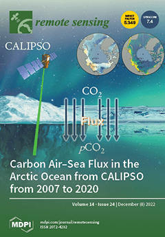
Quantified research on the Arctic Ocean carbon system is poorly understood, as it is limited by the scarce amount of available data. We represent the first-time spaceborne LiDAR data that were employed in research on the Arctic air–sea carbon cycle, thus providing enlarged data coverage and diurnal pCO2 variations. The CALIPSO measurements obtained through active LiDAR sensing are not limited by solar radiation, and thus, can provide “fill-in” data over the late autumn to early spring seasons, when ocean color sensors cannot record data. Therefore, we constructed the first complete record of polar pCO2. LiDAR measurements provide new measurements of ocean phytoplankton properties during both the daytime and nighttime, including in polar regions, thus improving our understanding of Arctic phytoplankton’s primary productivity and carbon fluxes. View this paper
  • Issues are regarded as officially published after their release is announced to the table of contents alert mailing list.
  • You may sign up for e-mail alerts to receive table of contents of newly released issues.
  • PDF is the official format for papers published in both, html and pdf forms. To view the papers in pdf format, click on the "PDF Full-text" link, and use the free Adobe Reader to open them.
Order results
Result details
Section
Select all
Export citation of selected articles as:
22 pages, 6259 KiB  
Article
A Hypered Deep-Learning-Based Model of Hyperspectral Images Generation and Classification for Imbalanced Data
by Hasan A. H. Naji, Tianfeng Li, Qingji Xue and Xindong Duan
Remote Sens. 2022, 14(24), 6406; https://doi.org/10.3390/rs14246406 - 19 Dec 2022
Cited by 6 | Viewed by 2932
Abstract
Recently, hyperspectral image (HSI) classification has become a hot topic in the geographical images research area. Sufficient samples are required for image classes to properly train classification models. However, a class imbalance problem has emerged in hyperspectral image (HSI) datasets as some classes [...] Read more.
Recently, hyperspectral image (HSI) classification has become a hot topic in the geographical images research area. Sufficient samples are required for image classes to properly train classification models. However, a class imbalance problem has emerged in hyperspectral image (HSI) datasets as some classes do not have enough samples for training, and some classes have many samples. Therefore, the performance of classifiers is likely to be biased toward the classes with the largest samples, and this can lead to a decrease in the classification accuracy. Therefore, a new deep-learning-based model is proposed for hyperspectral images generation and classification of imbalanced data. Firstly, the spectral features are extracted by a 1D convolutional neural network, whereas a 2D convolutional neural network extracts the spatial features and the extracted spatial features and spectral features are catenated into a stacked spatial–spectral feature vector. Secondly, an autoencoder model was developed to generate synthetic images for minority classes, and the image samples were balanced. The GAN model is applied to determine the synthetic images from the real ones and then enhancing the classification performance. Finally, the balanced datasets are fed to a 2D CNN model for performing classification and validating the efficiency of the proposed model. Our model and the state-of-the-art classifiers are evaluated by four open-access HSI datasets. The results showed that the proposed approach can generate better quality samples for rebalancing datasets, which in turn noticeably enhances the classification performance compared to the existing classification models. Full article
Show Figures

Graphical abstract

Graphical abstract
Full article ">Figure 1
<p>Architecture of the proposed model.</p>
Full article ">Figure 2
<p>The architecture of the feature extraction module.</p>
Full article ">Figure 3
<p>The data balancing module with autoencoder and GAN.</p>
Full article ">Figure 4
<p>The internal architecture of an encoder cell.</p>
Full article ">Figure 5
<p>The internal architecture of a decoder cell.</p>
Full article ">Figure 6
<p>The illustration of the discriminator network.</p>
Full article ">Figure 7
<p>Design of our classification network.</p>
Full article ">Figure 8
<p>Indian Pines dataset: (<b>a</b>) ground truth map; (<b>b</b>) pseudo color image.</p>
Full article ">Figure 9
<p>Salinas dataset: (<b>a</b>) ground truth map; (<b>b</b>) pseudo color image.</p>
Full article ">Figure 10
<p>(<b>a</b>) Ground truth map; (<b>b</b>) false color image of KSC.</p>
Full article ">Figure 11
<p>(<b>a</b>) Ground truth; (<b>b</b>) false color image for Botswana dataset.</p>
Full article ">Figure 12
<p>Classification maps of the real and synthetic Indian Pines dataset by classification models.</p>
Full article ">Figure 13
<p>Classification maps of the real and synthetic Salinas dataset by classification models.</p>
Full article ">Figure 14
<p>Classification maps of the real and synthetic KSC dataset by classification models.</p>
Full article ">Figure 15
<p>Classification maps of the real and synthetic Botswana dataset by classification models.</p>
Full article ">Figure 16
<p>Accuracy and loss convergence versus epochs of three models.</p>
Full article ">
17 pages, 5154 KiB  
Article
Surface Albedo and Snowline Altitude Estimation Using Optical Satellite Imagery and In Situ Measurements in Muz Taw Glacier, Sawir Mountains
by Fengchen Yu, Puyu Wang and Hongliang Li
Remote Sens. 2022, 14(24), 6405; https://doi.org/10.3390/rs14246405 - 19 Dec 2022
Cited by 3 | Viewed by 2475
Abstract
Glacier surface albedo strongly affects glacier mass balance by controlling the glacier surface energy budget. As an indicator of the equilibrium line altitude (ELA), the glacier snowline altitude (SLA) at the end of the melt season can reflect variations in the glacier mass [...] Read more.
Glacier surface albedo strongly affects glacier mass balance by controlling the glacier surface energy budget. As an indicator of the equilibrium line altitude (ELA), the glacier snowline altitude (SLA) at the end of the melt season can reflect variations in the glacier mass balance. Therefore, it is extremely crucial to investigate the changes of glacier surface albedo and glacier SLA for calculating and evaluating glacier mass loss. In this study, from 2011 to 2021, the surface albedo of the Muz Taw Glacier was derived from Landsat images with a spatial resolution of 30 m and from the Moderate Resolution Imaging Spectroradiometer albedo products (MOD10A1) with a temporal resolution of 1 day, which was verified through the albedo measured by the Automatic Weather Station (AWS) installed in the glacier. Moreover, the glacier SLA was determined based on the variation in the surface albedo, with the altitude change along the glacier main flowline derived from the Landsat image at the end of the melt season. The correlation coefficient of >0.7, with a risk of error lower than 5%, between the surface albedo retrieved from remote sensing images and the in situ measurement data indicated that the method of deriving the glacier surface albedo by the remote sensing method was reliable. The annual average albedo showed a slight upward trend (0.24%) from 2011 to 2021. A unimodal seasonal variation in albedo was demonstrated, with the downward trend from January to August and the upward trend from August to December. The spatial distribution of the albedo was not entirely dependent on altitude due to the dramatic effects of the topography and glacier surface conditions. The average SLA was 3446 m a.s.l., with a variation of 160 m from 2011 to 2021. The correlation analysis between the glacier SLA and annual mean temperature/annual precipitation demonstrated that the variations of the average SLA on the Muz Taw Glacier was primarily affected by the air temperature. This study improved our understanding of the ablation process and mechanism of the Muz Taw Glacier. Full article
Show Figures

Graphical abstract

Graphical abstract
Full article ">Figure 1
<p>(<b>a</b>) Location map of the study area with the red five-pointed star representing the Muz Taw Glacier in the Sawir Mountains, Central Asia. (<b>b</b>) Topography of the Muz Taw Glacier, with the distribution of ablation stakes and the AWS.</p>
Full article ">Figure 2
<p>The annual (<b>a</b>) and the seasonal variation (<b>b</b>) in surface albedo on the Muz Taw Glacier during 2011-2021. The blue bars represent the annual average glacier surface albedo anomalies. The red and black dots indicate the annual average glacier surface albedo and the surface albedo during ablation period (May to August), respectively, and the dotted line represents linear trend.</p>
Full article ">Figure 3
<p>Spatial distribution of glacier surface albedo derived from Landsat images near the melt season in the different periods.</p>
Full article ">Figure 4
<p>Variability in surface albedo along the glacier main flowline.</p>
Full article ">Figure 5
<p>The average albedo variation of the 50 m altitude intervals along the glacier main flowline in (<b>a</b>) 2019, (<b>b</b>) 2015, respectively.</p>
Full article ">Figure 6
<p>The average snowline altitude of the Muz Taw Glacier in the Sawir Mountains derived from Landsat over the period during 2011–2021.</p>
Full article ">Figure 7
<p>The scatter plots of the albedo values measured by the AWS against the values retrieved from Landsat images (<b>a</b>) and MOD10A1 (<b>b</b>). The relationship between the albedo derived from Landsat image and MOD10A1 albedo (<b>c</b>).</p>
Full article ">Figure 8
<p>Relationships between summer average albedo and annual glacier mass balance for the Muz Taw Glacier.</p>
Full article ">Figure 9
<p>Variations in the average air temperature and the precipitation from June to September. The red dots represent the air temperature, the light blue bars represent the total amount of precipitation, the dark blue bars represent the amount of solid precipitation, and the dotted line represents the linear trend.</p>
Full article ">Figure 10
<p>Average snowline altitude anomalies plotted versus air temperature anomalies (<b>a</b>) and solid precipitation anomalies (<b>b</b>) on the Muz Taw Glacier during 2011–2021.</p>
Full article ">Figure 11
<p>Spatial distribution of the average SLA in High Mountain Asia over the period of 2000–2021. The blue dots represent the average SLA of the glacier in the different regions.</p>
Full article ">
24 pages, 6412 KiB  
Article
Regional Satellite Algorithms to Estimate Chlorophyll-a and Total Suspended Matter Concentrations in Vembanad Lake
by Varunan Theenathayalan, Shubha Sathyendranath, Gemma Kulk, Nandini Menon, Grinson George, Anas Abdulaziz, Nick Selmes, Robert J. W. Brewin, Anju Rajendran, Sara Xavier and Trevor Platt
Remote Sens. 2022, 14(24), 6404; https://doi.org/10.3390/rs14246404 - 19 Dec 2022
Cited by 6 | Viewed by 4649
Abstract
A growing coastal population is leading to increased anthropogenic pollution that greatly affects coastal and inland water bodies, especially in the tropics. The Sustainable Development Goal-14, ‘Life below water’ emphasises the importance of conservation and sustainable use of the ocean and its resources. [...] Read more.
A growing coastal population is leading to increased anthropogenic pollution that greatly affects coastal and inland water bodies, especially in the tropics. The Sustainable Development Goal-14, ‘Life below water’ emphasises the importance of conservation and sustainable use of the ocean and its resources. Pollution management practices often include monitoring of water quality using in situ observations of chlorophyll-a (chl-a) and total suspended matter (TSM). Satellite technology, including the MultiSpectral Instrument (MSI) sensor onboard Sentinel-2, enables the continuous monitoring of these variables in inland waters at high spatial and temporal resolutions. To improve the monitoring of water quality in the tropical Vembanad-Kol-Wetland (VKW) system, situated on the southwest coast of India, we present two regionally tuned satellite algorithms developed to estimate chl-a and TSM concentrations. The new algorithms estimate the chl-a and TSM concentrations from the simulated reflectance values as a function of the inherent optical properties using a forward modelling approach. The model was parameterised using the National Aeronautics and Space Administration (NASA) bio-Optical Marine Algorithm Dataset (NOMAD) and in situ measurements collected in the VKW system. To assess model performance, results were compared with in situ measurements of chl-a and TSM and other existing satellite-based models of chl-a and TSM. For satellite application, two different atmospheric correction methods (ACOLITE and POLYMER) were tested and satellite matchups were used to validate the new chl-a and TSM algorithms following standard validation procedures. The results demonstrated that the new algorithms were in good agreement with in situ observations and outperform existing chl-a and TSM algorithms. The new regional satellite algorithms can be used to monitor water quality within the VKW system to support the sustainable management under natural (cyclones, floods, rainfall, and tsunami) and anthropogenic pressures (industrial effluents, agricultural practices, recreational activities, construction, and demolishing concrete structures) and help achieve Sustainable Development Goal 14. Full article
(This article belongs to the Section Ocean Remote Sensing)
Show Figures

Graphical abstract

Graphical abstract
Full article ">Figure 1
<p>The present study workflow of the satellite-derived chlorophyll-a (<math display="inline"><semantics> <mi>B</mi> </semantics></math>) and total suspended sediment (<math display="inline"><semantics> <mi>S</mi> </semantics></math>) concentrations in Vembanad Lake. In situ measurements from the Vembanad Lake and NOMAD datasets were used to model absorption and back-scattering coefficients to obtain model-derived reflectances (<math display="inline"><semantics> <mrow> <msub> <mi>R</mi> <mi>e</mi> </msub> </mrow> </semantics></math>). The <math display="inline"><semantics> <mrow> <msub> <mi>R</mi> <mi>e</mi> </msub> </mrow> </semantics></math> was then used to develop regional chlorophyll-a (<math display="inline"><semantics> <mi>B</mi> </semantics></math>) and total suspended matter (<math display="inline"><semantics> <mi>S</mi> </semantics></math>) algorithms. The <math display="inline"><semantics> <mrow> <msub> <mi>R</mi> <mi>e</mi> </msub> </mrow> </semantics></math> together with a satellite matchup dataset was used to correct satellite-derived (<math display="inline"><semantics> <mrow> <msub> <mi>ρ</mi> <mi>w</mi> </msub> </mrow> </semantics></math>) reflectance, which were obtained from the ACOLITE- and POLYMER-processed Sentinel-2 images. The bias-corrected satellite reflectance (<math display="inline"><semantics> <mrow> <msub> <mi>ρ</mi> <mi>w</mi> </msub> <msup> <mrow/> <mo>′</mo> </msup> </mrow> </semantics></math>) was used as input to the regional satellite-derived <math display="inline"><semantics> <mi>B</mi> </semantics></math> and <math display="inline"><semantics> <mi>S</mi> </semantics></math>.</p>
Full article ">Figure 2
<p>(<b>a</b>) Map showing the study site—Lake Vembanad with the locations of the 13 in situ sampling stations (with VL07 located in the tributary of River Murinjapuzha) and adjacent cities in Kerala; (<b>b</b>) the inset map shows the location of Lake Vembanad on the south-west coast of India.</p>
Full article ">Figure 3
<p>The relationship between the in situ back-scattering coefficient of non-algal suspended particles at 665 nm (<math display="inline"><semantics> <mrow> <msub> <mi>b</mi> <mrow> <mi>b</mi> <mi>S</mi> </mrow> </msub> <mfenced> <mrow> <mn>665</mn> </mrow> </mfenced> </mrow> </semantics></math>) and the in situ absorption coefficients of non-algal suspended particles (<math display="inline"><semantics> <mrow> <msub> <mi>a</mi> <mi>S</mi> </msub> <mfenced> <mrow> <mn>400</mn> </mrow> </mfenced> </mrow> </semantics></math>) obtained using the samples from the NOMAD dataset (<math display="inline"><semantics> <mrow> <mi>N</mi> <mo>=</mo> <mn>91</mn> </mrow> </semantics></math>) (<b>a</b>) and the comparison between the in situ and modelled <math display="inline"><semantics> <mrow> <msub> <mi>b</mi> <mrow> <mi>b</mi> <mi>S</mi> </mrow> </msub> <mfenced> <mrow> <mn>665</mn> </mrow> </mfenced> </mrow> </semantics></math> (<b>b</b>).</p>
Full article ">Figure 4
<p>Comparison between the in situ and modelled absorption coefficients of phytoplankton (<math display="inline"><semantics> <mrow> <msub> <mi>a</mi> <mi>B</mi> </msub> </mrow> </semantics></math>, <b>first column</b>), coloured dissolved organic matter (<math display="inline"><semantics> <mrow> <msub> <mi>a</mi> <mi>Y</mi> </msub> </mrow> </semantics></math>, <b>second column</b>), non-algal suspended particles (<math display="inline"><semantics> <mrow> <msub> <mi>a</mi> <mi>S</mi> </msub> <mo>,</mo> </mrow> </semantics></math> <b>third column</b>), and the sum of absorption by each of the constituents—<math display="inline"><semantics> <mi>B</mi> </semantics></math>, <math display="inline"><semantics> <mi>Y</mi> </semantics></math>, and <math display="inline"><semantics> <mi>S</mi> </semantics></math> and water, <math display="inline"><semantics> <mi>W</mi> </semantics></math>, (<math display="inline"><semantics> <mrow> <msub> <mi>a</mi> <mi>t</mi> </msub> </mrow> </semantics></math>, <b>forth column</b>) at five key wavelengths—443, 490, 560, 665, and 683 nm using the VL (green circles, <math display="inline"><semantics> <mrow> <mi>N</mi> <mo>=</mo> <mn>228</mn> </mrow> </semantics></math>) and NOMAD (grey circles, <math display="inline"><semantics> <mrow> <mi>N</mi> <mo>=</mo> <mn>839</mn> </mrow> </semantics></math>) datasets.</p>
Full article ">Figure 5
<p>Comparison between the in situ and modelled back-scattering coefficients (<math display="inline"><semantics> <mrow> <msub> <mi>b</mi> <mrow> <mi>b</mi> <mi>t</mi> </mrow> </msub> </mrow> </semantics></math>) at five key wavelengths—443, 490, 560, 665, and 683 nm using the NOMAD dataset (<math display="inline"><semantics> <mrow> <mi>N</mi> <mo>=</mo> <mn>111</mn> </mrow> </semantics></math>).</p>
Full article ">Figure 6
<p>Comparison between the measured and modelled reflectance. The grey circles show the comparison between the in situ (<math display="inline"><semantics> <mrow> <msub> <mi>R</mi> <mi>i</mi> </msub> </mrow> </semantics></math>) and modelled (<math display="inline"><semantics> <mrow> <msub> <mi>R</mi> <mi>e</mi> </msub> </mrow> </semantics></math>) reflectance using the NOMAD (<math display="inline"><semantics> <mrow> <mi>N</mi> <mo>=</mo> <mn>228</mn> </mrow> </semantics></math>) dataset at λ = 443, 490, 560, 665, and 683 nm. The faded red stars and blue triangles show the comparison between the uncorrected satellite-measured (<math display="inline"><semantics> <mrow> <msubsup> <mi>ρ</mi> <mi>w</mi> <mi>A</mi> </msubsup> </mrow> </semantics></math>, and <math display="inline"><semantics> <mrow> <msubsup> <mi>ρ</mi> <mi>w</mi> <mi>P</mi> </msubsup> </mrow> </semantics></math> for ACOLITE and POLYMER, respectively) and modelled reflectance; and the brighter red stars and blue triangles show the comparison between the corrected satellite-measured and modelled reflectance using the satellite matchup dataset (<math display="inline"><semantics> <mrow> <msubsup> <mi>ρ</mi> <mi>w</mi> <msup> <mi>A</mi> <mo>′</mo> </msup> </msubsup> </mrow> </semantics></math>, and <math display="inline"><semantics> <mrow> <msubsup> <mi>ρ</mi> <mi>w</mi> <msup> <mi>P</mi> <mo>′</mo> </msup> </msubsup> </mrow> </semantics></math>, with <math display="inline"><semantics> <mrow> <mi>N</mi> <mo>=</mo> <mn>12</mn> </mrow> </semantics></math> and <math display="inline"><semantics> <mrow> <mn>14</mn> </mrow> </semantics></math> for ACOLITE and POLYMER, respectively, at λ = 443, 490, 560, 665, and 705 nm). The statistical values in grey colour are estimated between the in situ and modelled reflectance, whereas the red (ACOLITE) and blue (POLYMER) coloured statistical values are estimated between the corrected satellite-measured and modelled reflectance.</p>
Full article ">Figure 7
<p>Comparison between the in situ and modelled <math display="inline"><semantics> <mi>B</mi> </semantics></math> (<b>a</b>–<b>d</b>) and <math display="inline"><semantics> <mi>S</mi> </semantics></math> (<b>e</b>–<b>g</b>) from various algorithms using the VL dataset (<math display="inline"><semantics> <mrow> <mi>N</mi> <mo>=</mo> <mn>162</mn> </mrow> </semantics></math>): O’Reilly et al. [<a href="#B33-remotesensing-14-06404" class="html-bibr">33</a>] (<b>a</b>), Gilerson et al. [<a href="#B36-remotesensing-14-06404" class="html-bibr">36</a>] (<b>b</b>), Gilerson et al. [<a href="#B36-remotesensing-14-06404" class="html-bibr">36</a>] (<b>c</b>) with tuned coefficients for VL, the algorithm using blue, green, and red reflectance based on multi-linear regression (<b>d</b>), Miller and McKee [<a href="#B38-remotesensing-14-06404" class="html-bibr">38</a>] (<b>e</b>), Nechad et al. [<a href="#B39-remotesensing-14-06404" class="html-bibr">39</a>] (<b>f</b>), and the algorithm using <math display="inline"><semantics> <mrow> <msub> <mi>R</mi> <mrow> <mi>r</mi> <mi>s</mi> </mrow> </msub> <mfenced> <mrow> <mn>665</mn> </mrow> </mfenced> </mrow> </semantics></math> equipped with exponential function (<b>g</b>). Note that algorithm results from c, d, and g were tuned for VL waters. Equations of all algorithms are provided in <a href="#remotesensing-14-06404-t002" class="html-table">Table 2</a>. The statistical values in black colour (black circles) are for <math display="inline"><semantics> <mrow> <mi>B</mi> <mo>&lt;</mo> <mn>20</mn> </mrow> </semantics></math> mg m<sup>−3</sup> and <math display="inline"><semantics> <mrow> <mi>S</mi> <mo>&lt;</mo> <mn>20</mn> </mrow> </semantics></math> g m<sup>−3</sup> and the ones in red colour (red triangles) are for <math display="inline"><semantics> <mrow> <mi>B</mi> <mo>≥</mo> <mn>20</mn> </mrow> </semantics></math> mg m<sup>−3</sup> and <math display="inline"><semantics> <mrow> <mi>S</mi> <mo>≥</mo> <mn>20</mn> </mrow> </semantics></math> g m<sup>−3</sup>.</p>
Full article ">Figure 8
<p>Comparison between the in situ and modelled <math display="inline"><semantics> <mi>B</mi> </semantics></math> (<b>a</b>,<b>b</b>) and <math display="inline"><semantics> <mi>S</mi> </semantics></math> (<b>c</b>,<b>d</b>) values using ACOLITE (red stars) and POLYMER (blue triangles) reflectance using the satellite matchup dataset (<math display="inline"><semantics> <mrow> <mi>N</mi> <mo>=</mo> <mn>12</mn> </mrow> </semantics></math> for ACOLITE and <math display="inline"><semantics> <mrow> <mi>N</mi> <mo>=</mo> <mn>14</mn> </mrow> </semantics></math> for POLYMER, <a href="#remotesensing-14-06404-t001" class="html-table">Table 1</a>). The black circles show the <math display="inline"><semantics> <mi>B</mi> </semantics></math> and <math display="inline"><semantics> <mi>S</mi> </semantics></math> values using modelled reflectance (<math display="inline"><semantics> <mrow> <msub> <mi>R</mi> <mi>e</mi> </msub> </mrow> </semantics></math>). The derived statistical values in black, blue, and red colours are generated between the in situ and modelled variables (<math display="inline"><semantics> <mi>B</mi> </semantics></math> and <math display="inline"><semantics> <mi>S</mi> </semantics></math>) using the modelled (<math display="inline"><semantics> <mrow> <msub> <mi>R</mi> <mi>e</mi> </msub> </mrow> </semantics></math>), and corrected ACOLITE (<math display="inline"><semantics> <mrow> <msubsup> <mi>ρ</mi> <mi>w</mi> <msup> <mi>A</mi> <mo>′</mo> </msup> </msubsup> </mrow> </semantics></math>) and POLYMER (<math display="inline"><semantics> <mrow> <msubsup> <mi>ρ</mi> <mi>w</mi> <msup> <mi>P</mi> <mo>′</mo> </msup> </msubsup> </mrow> </semantics></math>) reflectance, respectively.</p>
Full article ">Figure 9
<p>Maps showing the distribution of chlorophyll-a biomass based on the ACOLITE-processed data and total suspended matter based on the POLYMER-processed data for two Sentinel-2A images of Vembanad Lake dated on the 4th of January 2019 and the 25th of March 2019, respectively (<b>a</b>–<b>d</b>).</p>
Full article ">Figure A1
<p>The tuned correction coefficients <math display="inline"><semantics> <mrow> <msub> <mi>m</mi> <mi>A</mi> </msub> </mrow> </semantics></math> (ACOLITE) (<b>a</b>) and <math display="inline"><semantics> <mrow> <msub> <mi>m</mi> <mi>P</mi> </msub> </mrow> </semantics></math> (POLYMER) (<b>b</b>) that were used to correct for the difference between the satellite (<math display="inline"><semantics> <mrow> <msub> <mi>ρ</mi> <mi>w</mi> </msub> </mrow> </semantics></math>) and modelled reflectance <math display="inline"><semantics> <mrow> <msub> <mi>R</mi> <mi>e</mi> </msub> </mrow> </semantics></math>.</p>
Full article ">Figure A2
<p>The ranges of <math display="inline"><semantics> <mi>B</mi> </semantics></math> (<b>a</b>) and <math display="inline"><semantics> <mi>S</mi> </semantics></math> (<b>b</b>) from the NOMAD and Vembanad Lake datasets used in the present study. The dashed lines in both plots represent the ranges of <math display="inline"><semantics> <mi>B</mi> </semantics></math> (0.2~57 [mg m<sup>−3</sup>]) and <math display="inline"><semantics> <mi>S</mi> </semantics></math> (0.13~43.1 [g m<sup>−3</sup>]) used to derive <math display="inline"><semantics> <mrow> <msub> <mi>b</mi> <mrow> <mi>b</mi> <mi>S</mi> </mrow> </msub> <mfenced> <mrow> <mn>665</mn> </mrow> </mfenced> </mrow> </semantics></math> vs. <math display="inline"><semantics> <mi>S</mi> </semantics></math> relation [<a href="#B66-remotesensing-14-06404" class="html-bibr">66</a>].</p>
Full article ">Figure A3
<p>Spectral comparisons of modelled (<math display="inline"><semantics> <mrow> <msub> <mi>R</mi> <mi>e</mi> </msub> </mrow> </semantics></math> <b>first column</b>), uncorrected satellite-observed (<math display="inline"><semantics> <mrow> <msub> <mi>ρ</mi> <mi>w</mi> </msub> </mrow> </semantics></math>, <b>second column</b>), and corrected satellite-observed (<math display="inline"><semantics> <mrow> <msub> <mi>ρ</mi> <mi>w</mi> </msub> <msup> <mrow/> <mo>′</mo> </msup> </mrow> </semantics></math>, <b>third column</b>) reflectances. The insets show the reflectance spectra of <math display="inline"><semantics> <mrow> <msubsup> <mi>ρ</mi> <mi>w</mi> <mi>A</mi> </msubsup> </mrow> </semantics></math> (<b>b</b>) and <math display="inline"><semantics> <mrow> <msubsup> <mi>ρ</mi> <mi>w</mi> <mi>P</mi> </msubsup> </mrow> </semantics></math> (<b>e</b>) at smaller scales to demonstrate their actual magnitude and spectral features.</p>
Full article ">
2 pages, 174 KiB  
Correction
Correction: Jin et al. Influence of the Nocturnal Effect on the Estimated Global CO2 Flux. Remote Sens. 2022, 14, 3192
by Rui Jin, Tan Yu, Bangyi Tao, Weizeng Shao, Song Hu and Yongliang Wei
Remote Sens. 2022, 14(24), 6403; https://doi.org/10.3390/rs14246403 - 19 Dec 2022
Viewed by 1589
Abstract
We believe that several sentences in the description of the source (sink) changes of CO2 are prone to ambiguity and are not particularly well presented [...] Full article
(This article belongs to the Special Issue Advances on Land–Ocean Heat Fluxes Using Remote Sensing)
16 pages, 4280 KiB  
Technical Note
Load Estimation Based Dynamic Access Protocol for Satellite Internet of Things
by Mingchuan Yang, Guanchang Xue, Botao Liu, Yupu Yang and Yanyong Su
Remote Sens. 2022, 14(24), 6402; https://doi.org/10.3390/rs14246402 - 19 Dec 2022
Cited by 2 | Viewed by 1918
Abstract
In recent years, the Internet of Things (IoT) industry has become a research hotspot. With the advancement of satellite technology, the satellite Internet of Things is further developed along with a new generation of information technology and commercial markets. However, existing random access [...] Read more.
In recent years, the Internet of Things (IoT) industry has become a research hotspot. With the advancement of satellite technology, the satellite Internet of Things is further developed along with a new generation of information technology and commercial markets. However, existing random access protocols cannot cope with the access of a large number of sensors and short burst transmissions. The current satellite Internet of Things application scenarios are divided into two categories, one has only sensor nodes and no sink nodes, and the other has sink nodes. A time-slot random access protocol based on Walsh code is proposed for the satellite Internet-of-Things scenario with sink nodes. In this paper, the load estimation algorithm is used to reduce the resource occupancy rate in the case of medium and low load, and a dynamic Walsh code slot random access protocol is proposed to select the appropriate Walsh code length and frame length h. The simulation results show that the slotted random access protocol based on Walsh code can effectively improve the throughput of the system under high load. The introduction of load estimation in the case of medium and low load can effectively reduce the resource utilization of the system, and ensure that the performance of the access protocol based on Walsh codes does not deteriorate. However, in the case of high load, a large resource overhead is still required to ensure the access performance of the system. Full article
(This article belongs to the Special Issue Satellite and UAV for Internet of Things (IoT))
Show Figures

Figure 1

Figure 1
<p>Satellite IoT scenario model with sink nodes.</p>
Full article ">Figure 2
<p>Satellite IoT scenario model without sink nodes.</p>
Full article ">Figure 3
<p>The working principle of pure ALOHA.</p>
Full article ">Figure 4
<p>The working principle of slotted ALOHA.</p>
Full article ">Figure 5
<p>The working principle of CRDSA.</p>
Full article ">Figure 6
<p>Flowchart of the conflict resolution algorithm.</p>
Full article ">Figure 7
<p>User-side architecture design.</p>
Full article ">Figure 8
<p>On-board load architecture design.</p>
Full article ">Figure 9
<p>Throughput comparison curve under the same number of time slots.</p>
Full article ">Figure 10
<p>Comparison curve of PLR under the same number of time slots.</p>
Full article ">Figure 11
<p>Throughput performance curve of Walsh code time slot random access protocol with different parameters.</p>
Full article ">Figure 12
<p>PLR performance curve of Walsh code timeslot random access protocol with different parameters.</p>
Full article ">Figure 13
<p>Throughput performance simulation curve of the improved protocol.</p>
Full article ">Figure 14
<p>Simulation curve of packet loss rate performance of improved protocol.</p>
Full article ">Figure 15
<p>Resource occupancy of dynamic Walsh code slot random access protocol.</p>
Full article ">
16 pages, 2059 KiB  
Article
Effects of Inter- and Intra-Specific Interactions on Moose Habitat Selection Limited by Temperature
by Heng Bao, Penghui Zhai, Dusu Wen, Weihua Zhang, Ye Li, Feifei Yang, Xin Liang, Fan Yang, Nathan J. Roberts, Yanchun Xu and Guangshun Jiang
Remote Sens. 2022, 14(24), 6401; https://doi.org/10.3390/rs14246401 - 19 Dec 2022
Cited by 3 | Viewed by 2422
Abstract
Habitat selection and daily activity patterns of large herbivores might be affected by inter- and intra-specific interaction, changes of spatial scale, and seasonal temperature. To reveal what factors were driving the habitat selection of moose, we collected moose (Alces alces) and [...] Read more.
Habitat selection and daily activity patterns of large herbivores might be affected by inter- and intra-specific interaction, changes of spatial scale, and seasonal temperature. To reveal what factors were driving the habitat selection of moose, we collected moose (Alces alces) and roe deer (Capreolus pygargus bedfordi) occurrence data, analyzed the multi-scale habitat selection and daily activity patterns of moose, and quantified the effects of spatial heterogeneity distribution of temperature, as well as the occurrence of roe deer on these habitat selection processes. Our results suggested that moose and roe deer distribution spatially overlap and that moose habitat selection is especially sensitive to landscape variables at large scales. We also found that the activity patterns of both sexes of moose had a degree of temporal separation with roe deer. In the snow-free season, temperatures drove moose habitat selection to be limited by threshold temperatures of 17 °C; in the snowy season, there were no similar temperature driving patterns, due to the severe cold environment. The daily activity patterns of moose showed seasonal change, and were more active at dawn and nightfall to avoid heat pressure during the snow-free season, but more active in the daytime for cold adaptation to the snow season. Consequently, this study provides new insights on how the comprehensive effects of environmental change and inter- and intra- specific relationships influence the habitat selection and daily activity patterns of moose and other heat sensitive animals with global warming. Full article
(This article belongs to the Special Issue Camera Trapping for Animal Ecology and Conservation)
Show Figures

Graphical abstract

Graphical abstract
Full article ">Figure 1
<p>Camera trap points in Hanma National Nature Reserve, Inner Mongolia, China.</p>
Full article ">Figure 2
<p>Contribution rate of female and male moose habitat parameters in the most parsimonious univariate models during the snow-free and snow seasons, including elevation (<b>a</b>), larch forest (<b>b</b>), mixed forest (<b>c</b>) and <span class="html-italic">Betula exilis</span> shrub (<b>d</b>). Males in the snow season (SM), females in the snow season (SF), males in the snow-free season (NM), females in the snow-free season (NF). “+” indicates a positive relationship, “−” indicates a negative relationship, and no symbol indicates no significant relationship, “NA indicates not applicable”.</p>
Full article ">Figure 3
<p>Spatial overlap relationships of female and male moose with roe deer created by modelling the occurrence frequency during the snow−free and snow time periods/seasons; including the spatial overlap of male moose and female moose during snow−free (<b>a</b>) and snow periods (<b>b</b>), male moose and roe deer during snow−free (<b>c</b>) and snow periods (<b>d</b>), female moose and roe deer during snow−free (<b>e</b>) and snow periods (<b>f</b>).</p>
Full article ">Figure 4
<p>Temporal overlap of daily activity patterns of female and male moose during the snow−free and snow time periods/seasons, and the respective overlap with roe deer during both time periods; including the temporal overlap of male moose and female moose during snow−free (<b>a</b>) and snow periods (<b>b</b>), male moose and roe deer during snow−free (<b>c</b>) and snow periods (<b>d</b>), female moose and roe deer during snow−free (<b>e</b>) and snow periods (<b>f</b>).</p>
Full article ">Figure 5
<p>Temperature of moose occurrence points in each month, showing that moose occurred at temperatures above the threshold of 14 °C (Tre 1) during summer (during snow−free period), and that moose occurrence did not transgress the upper threshold of 17 °C (Tre 2) during summer (snow−free period). The gray dotted line showed moose occurred at temperatures lower than the −5 °C in winter (during snow period).</p>
Full article ">Figure 6
<p>Relationships between female (<b>a</b>,<b>c</b>) and male (<b>b</b>,<b>d</b>) moose encounter frequency and local temperature (°C) at camera trap points during the snow−free and snow time periods/seasons.</p>
Full article ">
20 pages, 2770 KiB  
Article
Spatial Downscaling of NPP-VIIRS Nighttime Light Data Using Multiscale Geographically Weighted Regression and Multi-Source Variables
by Shangqin Liu, Xizhi Zhao, Fuhao Zhang, Agen Qiu, Liujia Chen, Jing Huang, Song Chen and Shu Zhang
Remote Sens. 2022, 14(24), 6400; https://doi.org/10.3390/rs14246400 - 19 Dec 2022
Cited by 11 | Viewed by 3887
Abstract
Remote sensing images of nighttime lights (NTL) were successfully used at global and regional scales for various applications, including studies on population, politics, economics, and environmental protection. The Suomi National Polar-orbiting Partnership with the Visible Infrared Imaging Radiometer Suite (NPP-VIIRS) NTL data has [...] Read more.
Remote sensing images of nighttime lights (NTL) were successfully used at global and regional scales for various applications, including studies on population, politics, economics, and environmental protection. The Suomi National Polar-orbiting Partnership with the Visible Infrared Imaging Radiometer Suite (NPP-VIIRS) NTL data has the advantages of high temporal resolution, long coverage time series, and wide spatial range. The spatial resolution of the monthly and annual composite data of NPP-VIIRS NTL is only 500 m, which hinders studies requiring higher resolution. We propose a multi-source spatial variable and Multiscale Geographically Weighted Regression (MGWR)-based method to achieve the downscaling of NPP-VIIRS NTL data. An MGWR downscaling framework was implemented to obtain NTL data at 120 m resolution based on auxiliary data representing socioeconomic or physical geographic attributes. The downscaled NTL data were validated against LuoJia1-01 imagery based on the coefficient of determination (R2) and the root-mean-square error (RMSE). The results suggested that the spatial resolution of the data was enhanced after downscaling, and the MGWR-based downscaling results demonstrated higher R2 (R2 = 0.9141) and lower RMSE than those of Geographically Weighted Regression and Random Forest-based algorithms. Additionally, MGWR can reveal the different relationships between multiple auxiliary and NTL data. Therefore, this study demonstrates that the spatial resolution of NPP-VIIRS NTL data is improved from 500 m to 120 m upon downscaling, thereby facilitating NTL-based applications. Full article
Show Figures

Figure 1

Figure 1
<p>Map of the study areas (zoomed-in Beijing city center, red voxes) and NTL datasets. (<b>a</b>,<b>b</b>) Overall spatial distributions of the NPP-VIIRS NTL data (September 2018) and LuoJia1-01 NTL data (September 2018).</p>
Full article ">Figure 2
<p>The proposed methodology for spatial downscaling of NTL data using MGWR.</p>
Full article ">Figure 3
<p>Scatter density plots between the estimated and actual NTL values for each pixel between (<b>a</b>) MGWR, (<b>b</b>) GWR, and the (<b>c</b>) RF regression.</p>
Full article ">Figure 4
<p>Spatial images showing the comparison of the results of the three downscaling methods in the zoomed-in Beijing city center, (<b>a</b>) LuoJia-01, (<b>b</b>) NPP/VIIRS, (<b>c</b>) MGWR, (<b>d</b>) GWR, (<b>e</b>) RF. (Spatial resolution: 500 m; study period: September 2018).</p>
Full article ">Figure 5
<p>Spatial texture contrast maps of the downscaled NTL data predicted by the three methods. The red boxes indicate the location of the local area within the entire study area. (<b>a</b>) Beijing Capital International Airport; (<b>b</b>) part of Central Beijing. Study period: September 2018.</p>
Full article ">Figure 6
<p>Maps depicting the validation areas (HR and FS) and NTL datasets. (<b>a</b>,<b>b</b>) Overall spatial distributions of the NPP-VIIRS NTL data (September 2018) and LuoJia1-01 NTL data (September 2018).</p>
Full article ">Figure 7
<p>Spatial images comparing of the results of the three downscaling methods in the HR region, (<b>a</b>) LuoJia-01, (<b>b</b>) NPP/VIIRS, (<b>c</b>) MGWR, (<b>d</b>) GWR, (<b>e</b>) RF. (Spatial resolution: 500 m; study period: September 2018).</p>
Full article ">Figure 8
<p>Spatial images comparing results of the three downscaling methods in the FS region, (<b>a</b>) LuoJia-01, (<b>b</b>) NPP/VIIRS, (<b>c</b>) MGWR, (<b>d</b>) GWR, (<b>e</b>) RF. (Spatial resolution: 500 m; study period: September 2018).</p>
Full article ">
20 pages, 3377 KiB  
Article
An In-Depth Assessment of the Drivers Changing China’s Crop Production Using an LMDI Decomposition Approach
by Yuqiao Long, Wenbin Wu, Joost Wellens, Gilles Colinet and Jeroen Meersmans
Remote Sens. 2022, 14(24), 6399; https://doi.org/10.3390/rs14246399 - 19 Dec 2022
Cited by 3 | Viewed by 2454
Abstract
Over the last decades, growing crop production across China has had far-reaching consequences for both the environment and human welfare. One of the emerging questions is “how to meet the growing food demand in China?” In essence, the consensus is that the best [...] Read more.
Over the last decades, growing crop production across China has had far-reaching consequences for both the environment and human welfare. One of the emerging questions is “how to meet the growing food demand in China?” In essence, the consensus is that the best way forward would be to increase crop yield rather than further extend the current cropland area. However, assessing progress in crop production is challenging as it is driven by multiple factors. To date, there are no studies to determine how multiple factors affect the crop production increase, considering both intensive farming (using yield and multiple cropping index) and large-scale farming (using mean parcel size and number of parcels). Using the Logarithmic-Mean-Divisia-Index (LMDI) decomposition method combined with statistical data and land cover data (GlobeLand30), we assess the contribution of intensive farming and large-scale farming changes to crop production dynamics at the national and county scale. Despite a negative contribution from MPS (mean parcel size, ), national crop production increased due to positive contributions from yield (), MCI (multiple cropping index, ), as well as NP (number of parcels, ). This allowed China to meet the growing national crop demand. We further find that large differences across regions persist over time. For most counties, the increase in crop production is a consequence of improved yields. However, in the North China Plain, NP is another important factor leading to crop production improvement. On the other hand, regions witnessing a decrease in crop production (e.g., the southeast coastal area of China) were characterized by a remarkable decrease in yield and MCI. Our detailed analyses of crop production provide accurate estimates and therefore can guide policymakers in addressing food security issues. Specifically, besides stabilizing yield and maintaining the total NP, it would be advantageous for crop production to increase the mean parcel size and MCI through land consolidation and financial assistance for land transfer and advanced agricultural infrastructure. Full article
(This article belongs to the Special Issue Monitoring Agricultural Land-Use Change and Land-Use Intensity Ⅱ)
Show Figures

Graphical abstract

Graphical abstract
Full article ">Figure 1
<p>Digital elevation model (<b>a</b>) and climate zones of China (<b>b</b>) with annotation of the provinces.</p>
Full article ">Figure 2
<p>Spatial pattern of cropland in GlobeLand30 ((<b>a</b>): 2000, (<b>b</b>): 2000–2010). Note that the overall accuracy of GlobeLand30 in China has reached 80%, including the cropland layer. The maps were generated using ArcGIS 10.2 ESRI (Environmental Systems Research Institute, 2013).</p>
Full article ">Figure 3
<p>Flowchart of the methodological approach. Our study approach comprises the following steps: (1) Extracting cropland layer from GlobeLand30 and calculating landscape metrics using FRAGSTATS 4.2; (2) Calculating crop yield and multiple cropping index at the county scale based on statistical data; (3) Quantifying the contributions of all four indicators to crop production change, including food, feed, and fiber crops (cylinders = datasets, diamonds = data-processing and method, rectangular = results and maps).</p>
Full article ">Figure 4
<p>Characterization of change in four factors ((<b>a</b>): yield, (<b>b</b>): multiple cropping index (<span class="html-italic">MCI</span>), (<b>c</b>): mean parcel size (<span class="html-italic">MPS</span>), (<b>d</b>): number of parcels (NP)) at the county scale across China between 2000 and 2010.</p>
Full article ">Figure 5
<p>Map of crop production change at the county scale across China. The bar chart shows the proportion of the counties characterized by a given change in crop production corresponding to the intervals displayed in the legend of the map.</p>
Full article ">Figure 6
<p>Factor decomposition of the total change in crop production across China between 2000 and 2010, considering the contributions of yield (∆G<sub>yield</sub>), multiple cropping index (<span class="html-italic">MCI</span>, ∆G<sub><span class="html-italic">MCI</span></sub>), number of parcels (NP, ∆G<sub>NP</sub>), and mean parcel size (<span class="html-italic">MPS</span>, ∆G<sub><span class="html-italic">MPS</span></sub>).</p>
Full article ">Figure 7
<p>Decomposition of changes in China’s crop production at the county scale with the individual contributions of the factors being given in the subpanels, (<b>a</b>): Yield, (<b>b</b>): Multiple Cropping Index (<span class="html-italic">MCI</span>), (<b>c</b>): Mean Parcel Size (<span class="html-italic">MPS</span>), (<b>d</b>): Number of Parcels (NP).</p>
Full article ">Figure 8
<p>Spatial pattern of the dominant factors influencing crop production in China. Colors represent the dominant factor, whereas hatching indicates the overall crop production trend (i.e., “+” is net increase and “−” is net decrease in crop production).</p>
Full article ">
21 pages, 4938 KiB  
Article
Drought Monitoring and Performance Evaluation Based on Machine Learning Fusion of Multi-Source Remote Sensing Drought Factors
by Yangyang Zhao, Jiahua Zhang, Yun Bai, Sha Zhang, Shanshan Yang, Malak Henchiri, Ayalkibet Mekonnen Seka and Lkhagvadorj Nanzad
Remote Sens. 2022, 14(24), 6398; https://doi.org/10.3390/rs14246398 - 19 Dec 2022
Cited by 25 | Viewed by 6881
Abstract
Drought is an extremely dangerous natural hazard that causes water crises, crop yield reduction, and ecosystem fires. Researchers have developed many drought indices based on ground-based climate data and various remote sensing data. Ground-based drought indices are more accurate but limited in coverage; [...] Read more.
Drought is an extremely dangerous natural hazard that causes water crises, crop yield reduction, and ecosystem fires. Researchers have developed many drought indices based on ground-based climate data and various remote sensing data. Ground-based drought indices are more accurate but limited in coverage; while the remote sensing drought indices cover larger areas but have poor accuracy. Applying data-driven models to fuse multi-source remote sensing data for reproducing composite drought index may help fill this gap and better monitor drought in terms of spatial resolution. Machine learning methods can effectively analyze the hierarchical and non-linear relationships between the independent and dependent variables, resulting in better performance compared with traditional linear regression models. In this study, seven drought impact factors from the Moderate Resolution Imaging Spectroradiometer (MODIS) satellite sensor, Global Precipitation Measurement Mission (GPM), and Global Land Data Assimilation System (GLDAS) were used to reproduce the standard precipitation evapotranspiration index (SPEI) for Shandong province, China, from 2002 to 2020. Three machine learning methods, namely bias-corrected random forest (BRF), extreme gradient boosting (XGBoost), and support vector machines (SVM) were applied as regression models. Then, the best model was used to construct the spatial distribution of SPEI. The results show that the BRF outperforms XGBoost and SVM in SPEI estimation. The BRF model can effectively monitor drought conditions in areas without ground observation data. The BRF model provides comprehensive drought information by producing a spatial distribution of SPEI, which provides reliability for the BRF model to be applied in drought monitoring. Full article
Show Figures

Figure 1

Figure 1
<p>Location and land cover types of the study area in Shandong province.</p>
Full article ">Figure 2
<p>Workflow of this study.</p>
Full article ">Figure 3
<p>Scatterplot of model predictions vs. observations. (<b>a</b>,<b>c</b>,<b>e</b>) is the performance of BRF, SVM, and XGBoost on the training set. (<b>b</b>,<b>d</b>,<b>f</b>) is the performance of BRF, SVM, and XGBoost on the test set. “**” represents the significance level of the experiment is greater than 0.99.</p>
Full article ">Figure 4
<p>Boxplots of model performance measurements ((<b>a</b>). coefficient of determination and (<b>b</b>). root mean squared error) for prediction of SPEI.</p>
Full article ">Figure 5
<p>Comparation among SPEI−3 calculated from observations and forecasted by BRF, XGBoost, and SVM approaches at four stations in Shandong province, China.</p>
Full article ">Figure 6
<p>Pearson correlation coefficients of SPEI-3 with drought impact factors. The “1” and “3” suffixes following the variable name represent the average of one-month and three-month time scales.</p>
Full article ">Figure 7
<p>The change of SPEI−3 in Shandong province from 2002 to 2020.</p>
Full article ">Figure 8
<p>SPEI-3 spatial distribution simulated by the BRF model and the site’s drought distribution in a drought year (2002).</p>
Full article ">Figure 9
<p>SPEI-3 spatial distribution simulated by the BRF model and the site’s drought distribution in a drought year (2006).</p>
Full article ">Figure 10
<p>SPEI-3 spatial distribution simulated by the BRF model and the site’s drought distribution in a drought year (2011).</p>
Full article ">
20 pages, 5220 KiB  
Article
Development and Assessment of Seasonal Rainfall Forecasting Models for the Bani and the Senegal Basins by Identifying the Best Predictive Teleconnection
by Luis Balcázar, Khalidou M. Bâ, Carlos Díaz-Delgado, Miguel A. Gómez-Albores, Gabriel Gaona and Saula Minga-León
Remote Sens. 2022, 14(24), 6397; https://doi.org/10.3390/rs14246397 - 19 Dec 2022
Viewed by 2592
Abstract
The high variability of rainfall in the Sahel region causes droughts and floods that affect millions of people every year. Several rainfall forecasting models have been proposed, but the results still need to be improved. In this study, linear, polynomial, and exponential models [...] Read more.
The high variability of rainfall in the Sahel region causes droughts and floods that affect millions of people every year. Several rainfall forecasting models have been proposed, but the results still need to be improved. In this study, linear, polynomial, and exponential models are developed to forecast rainfall in the Bani and Senegal River basins. All three models use Atlantic sea surface temperature (SST). A fourth algorithm using stepwise regression was also developed for the precipitation estimates over these two basins. The stepwise regression algorithm uses SST with covariates, mean sea level pressure (MSLP), relative humidity (RHUM), and five El Niño indices. The explanatory variables SST, RHUM, and MSLP were selected based on principal component analysis (PCA) and cluster analysis to find the homogeneous region of the Atlantic with the greatest predictive ability. PERSIANN-CDR rainfall data were used as the dependent variable. Models were developed for each pixel of 0.25° × 0.25° spatial resolution. The second-order polynomial model with a lag of about 11 months outperforms all other models and explains 87% of the variance in precipitation over the two watersheds. Nash–Sutcliffe efficiency (NSE) values were between 0.751 and 0.926 for the Bani River basin and from 0.175 to 0.915 for the Senegal River basin, for which the lowest values are found in the driest area (Sahara). Results showed that the North Atlantic SST shows a more robust teleconnection with precipitation dynamics in both basins. Full article
Show Figures

Figure 1

Figure 1
<p>Location of the basins of the Bani River at Beneny Kegny (upper Niger) and the Senegal River at Bakel on a digital elevation model (DEM). Location of rain gauges (blue dots) and buoys in the Atlantic located off the coast of West Africa (magenta boxes) and the Sahel region (yellow stripe).</p>
Full article ">Figure 2
<p>Classification of the Tropical Atlantic into homogeneous regions, using PCA and cluster analysis: SST1, SST2, SST3, RHUM1, RHUM2, RHUM3, MSLP1, and MSLP2.</p>
Full article ">Figure 3
<p>Spatial distribution of models that best reproduce rainfall in each pixel of the Bani and Senegal River basins.</p>
Full article ">Figure 4
<p>Spatial distribution of NSE with the polynomial model in the 3 SST regions of the Atlantic and their respective time lags (5 months for SST1, 10 months for SST2, and 11 months for SST3).</p>
Full article ">Figure 5
<p>Spatial-seasonal distribution of rainfall forecast with the polynomial model, sample from the years 2005 to 2020.</p>
Full article ">Figure 6
<p>Comparison between the forecast for 2021 and PERSIANN-CDR monthly rainfall (mm) using the monthly frequency hyetograph (MFH) of the pixel where the rain gauge is located.</p>
Full article ">Figure 7
<p>Classification of the seasonal rainfall forecast for 2021 over the Bani River and Senegal River watersheds in terms of wet, normal, and dry.</p>
Full article ">
22 pages, 5581 KiB  
Article
An Improved Exponential Model Considering a Spectrally Effective Moisture Threshold for Proximal Hyperspectral Reflectance Simulation and Soil Salinity Estimation
by Xi Huang, Tiecheng Bai, Huade Guan, Xiayong Wei, Yali Wang and Xiaomin Mao
Remote Sens. 2022, 14(24), 6396; https://doi.org/10.3390/rs14246396 - 18 Dec 2022
Cited by 1 | Viewed by 2555
Abstract
Soil salinization has become one of the main factors restricting sustainable development of agriculture. Field spectrometry provides a quick way to predict the soil salinization. However, soil moisture content (SMC) seriously interferes with the spectral information of saline soil in arid areas. It [...] Read more.
Soil salinization has become one of the main factors restricting sustainable development of agriculture. Field spectrometry provides a quick way to predict the soil salinization. However, soil moisture content (SMC) seriously interferes with the spectral information of saline soil in arid areas. It is vital to establish a model that is insensitive to SMC for potential in situ field applications. The soil spectral reflectance exponential model (SSREM) has been widely employed for reflectance simulation and SSC inversion. However, its reliability for saline soils with high SMC has not been verified yet. Based on hyperspectral remote sensing data (400~1000 nm) on 459 saline soil samples in Shiyang River Basin of Northwest China, we investigated the role of SMC and SSC in soil spectral reflectance from 29 October 2020 to 22 January 2021. Targeted at saline soils, soil spectral moisture threshold (MT) was introduced to improve the SSREM toward a modified spectral reflectance exponential model (MT-SSREM). The bands that are sensitive to SSC but not sensitive to SMC were obtained based on a method of correlation analysis between original spectra, four kinds of spectral data, and SSC. SSREM and MT-SSREM were finally applied to inversely estimate SSC. Results show that wavelengths at 658~660, 671~685, 938 nm were suitable for SSC estimation. Furthermore, although SSREM was able to simulate the spectral reflectance of most saline soils, its simulation accuracy was low for saline soil samples with high SMC (SMC > MT(i), 400 nmi1000 nm), while MT-SSREM performed well over the whole range of SMC. The simulated spectral reflectance from MT-SSREM agreed well with the measured reflectance, with the R2 being generally larger than 0.9 and RMSE being less than 0.1. More importantly, MT-SSREM performed substantially better than SSREM for SSC estimation; in the statistical performance of the former case, R2 was in range of 0.60~0.66, RMSE was in range of 0.29~0.33 dS m−1; in the latter case, R2 was in range of 0.10~0.16, RMSE was in the range of 0.26~0.29 dS m−1. MT-SSREM proposed in this study thus provides a new direction for estimating hyperspectral reflectance and SSC under various soil moisture conditions at wavelengths from 400 to 1000 nm. It also provides an approach for SSC and SMC mapping in salinization regions by incorporating remote sensing data, such as GF-5. Full article
(This article belongs to the Section Remote Sensing Image Processing)
Show Figures

Figure 1

Figure 1
<p>Map of the study area.</p>
Full article ">Figure 2
<p>Study framework. Note: RSR is raw reflectance spectra reflectance; SSREM is the soil spectral reflectance exponential model; MT is the moisture threshold; MT-SSREM is the modified model based on SSREM considering MT; FD is the first derivative of RSR; SD is the second derivative of RSR; MSC is the multiplicative scatter correction of RSR; SNV is the standard normal variate transform of RSR.</p>
Full article ">Figure 3
<p>The workflow of splitting the validation and calibration datasets.</p>
Full article ">Figure 4
<p>The distribution and correlation between each pair of four cation concentrations (g kg<sup>−1</sup>) in soil samples. Note: ** marks a significant correlation at a level of <span class="html-italic">p</span> &lt; 0.01.</p>
Full article ">Figure 5
<p>The relationship between SSC and spectral reflectance: (<b>a</b>) variation of spectral reflectance of soil with SSC with SMC 0.11 g g<sup>−1</sup>; (<b>b</b>) correlation analysis of SSC with reflectance and log(reflectance), respectively.</p>
Full article ">Figure 6
<p>Variation of spectral reflectance of soils with SMC under three SSC conditions: (<b>a</b>) SSC 0.15 dS m<sup>−1</sup>, (<b>b</b>) SSC 0.50 dS m<sup>−1</sup> and (<b>c</b>) SSC 1.6 dS m<sup>−1</sup>.</p>
Full article ">Figure 7
<p>The correlation coefficients of five kinds of spectral data with SMC (<b>a</b>–<b>e</b>) and SSC (<b>f</b>–<b>j</b>) under different preprocessing methods. (<b>a</b>,<b>f</b>) raw spectral reflectance; (<b>b</b>,<b>g</b>) first derivative; (<b>c</b>,<b>h</b>) second derivative; (<b>d</b>,<b>i</b>) multiplicative scatter correction; (<b>e</b>,<b>j</b>) standard normal transformation.</p>
Full article ">Figure 8
<p>Relationship between SMC and spectral reflectance: (<b>a</b>) fitting R<sup>2</sup> of spectral reflectance and SMC by different functions; (<b>b</b>) spectral reflectance variation with SMC at the wavelength 400 and 650 nm; (<b>c</b>) MT value of each band.</p>
Full article ">Figure 9
<p>Calibration results of parameters <span class="html-italic">a</span>, <span class="html-italic">b</span> and <span class="html-italic">R</span><sub>0</sub> in the soil spectral reflectance exponential model: (<b>a</b>) parameters <span class="html-italic">a</span> and <span class="html-italic">b</span>; (<b>b</b>) <span class="html-italic">R</span><sub>0</sub>.</p>
Full article ">Figure 10
<p>Comparison of simulated reflectance based on SSREM with measured reflectance: (<b>a</b>) simulation accuracy of calibration dataset; (<b>b</b>) simulation accuracy of validation dataset; (<b>c</b>–<b>e</b>) measurement and simulation of wet-soil reflectance from calibration dataset and (<b>f</b>–<b>h</b>) from validation dataset.</p>
Full article ">Figure 10 Cont.
<p>Comparison of simulated reflectance based on SSREM with measured reflectance: (<b>a</b>) simulation accuracy of calibration dataset; (<b>b</b>) simulation accuracy of validation dataset; (<b>c</b>–<b>e</b>) measurement and simulation of wet-soil reflectance from calibration dataset and (<b>f</b>–<b>h</b>) from validation dataset.</p>
Full article ">Figure 11
<p>Comparison of simulated reflectance based on MT-SSREM with measured reflectance: (<b>a</b>) simulation accuracy of calibration dataset; (<b>b</b>) simulation accuracy of validation dataset; (<b>c</b>–<b>e</b>) measurement and simulation of wet-soil reflectance from calibration dataset and (<b>f</b>–<b>h</b>) from validation dataset.</p>
Full article ">Figure 12
<p>Performance of suggested bands to estimate SSC based on MT-SSREM and SSREM. (<b>a</b>–<b>t</b>) 658~660, 672~685, 938, 939 and 961 nm.</p>
Full article ">Figure 13
<p>First derivative of reflectance.</p>
Full article ">
23 pages, 35978 KiB  
Article
Comprehensive Evaluation of Data-Related Factors on BDS-3 B1I + B2b Real-Time PPP/INS Tightly Coupled Integration
by Junyao Kan, Zhouzheng Gao, Qiaozhuang Xu, Ruohua Lan, Jie Lv and Cheng Yang
Remote Sens. 2022, 14(24), 6395; https://doi.org/10.3390/rs14246395 - 18 Dec 2022
Cited by 2 | Viewed by 2087
Abstract
Owing to the developments of satellite-based and network-based real-time satellite precise products, the Precise Point Positioning (PPP) technique has been applied far and wide, especially since the PPP-B2b service was provided by the third-generation BeiDou Navigation Satellite System (BDS-3). However, satellite outages during [...] Read more.
Owing to the developments of satellite-based and network-based real-time satellite precise products, the Precise Point Positioning (PPP) technique has been applied far and wide, especially since the PPP-B2b service was provided by the third-generation BeiDou Navigation Satellite System (BDS-3). However, satellite outages during dynamic application lead to significant degradation of the accuracy and continuity of PPP. A generally used method is integrating PPP with Inertial Measurement Units (IMUs) to enhance positioning performance. Previous works on this topic are usually based on IMU data at a high sampling rate and are mostly implemented in post-processing mode. This paper will carry out a compressive assessment of the impacts of different types of precise satellite products (real-time products from the CAS, DLR, GFZ, WHU, and the final one from GFZ), Doppler observations, and different sampling rates of IMU data on the performance of the tightly coupled integration of the BDS-3 B1I/B2b and the Inertial Navigation System (INS). Results based on a group of on-board experimental data illustrate that (1) the positioning accuracy with products supplied by the CAS and WHU are roughly consistent with those using the final products; (2) the Doppler observations can effectively improve the accuracies of velocity, attitude, and vertical position at the initial epochs and during the reconvergence periods, but have invisible influences on the overall positioning, velocity, and attitude determination; and (3) the impact of IMU data interval on the performance of PPP/INS tightly coupled integration is insignificant when there are enough available satellites. However, the divergent speed of position is visibly affected by the IMU sampling rate during satellite outage periods. Full article
(This article belongs to the Special Issue Advances in Beidou/GNSS High Precision Positioning and Navigation)
Show Figures

Figure 1

Figure 1
<p>Trajectory of the vehicle test.</p>
Full article ">Figure 2
<p>Number of available satellites and the corresponding PDOP.</p>
Full article ">Figure 3
<p>Position differences of PPP, PPP/INS TCI, and TCI-RKF: (<b>a</b>) position differences of BDS-3 PPP, TCI, and TCI-RKF; (<b>b</b>) position differences of GPS PPP, TCI, and TCI-RKF.</p>
Full article ">Figure 4
<p>Position differences of BDS-3 PPP/INS TCI (<b>a</b>) and GPS PPP/INS TCI (<b>b</b>) with different orbit and clock products.</p>
Full article ">Figure 5
<p>Satellite numbers and PDOP values with DLR products.</p>
Full article ">Figure 6
<p>Position error CDF of BDS-3 PPP/INS TCI (<b>a</b>) and GPS PPP/INS TCI (<b>b</b>) with different orbit and clock products.</p>
Full article ">Figure 7
<p>Position offsets of the BDS-3/GPS TCI in modes of dmode0 (with Doppler) and dmode1 (without Doppler).</p>
Full article ">Figure 8
<p>The max position errors of the BDS-3/GPS TCI in modes of dmode0 (with Doppler) and dmode1 (without Doppler).</p>
Full article ">Figure 9
<p>Velocity offsets of the BDS-3/GPS TCI in modes of dmode0 (with Doppler) and dmode1 (without Doppler).</p>
Full article ">Figure 10
<p>The max velocity errors of the BDS-3/GPS TCI in modes of dmode0 (with Doppler) and dmode1 (without Doppler).</p>
Full article ">Figure 11
<p>Attitude offsets of the BDS-3/GPS TCI in modes of dmode0 (with Doppler) and dmode1 (without Doppler).</p>
Full article ">Figure 12
<p>The max attitude errors of the BDS-3/GPS TCI in modes of dmode0 (with Doppler) and dmode1 (without Doppler).</p>
Full article ">Figure 13
<p>Average and max convergence time of the BDS-3 TCI (<b>left</b>) and GPS TCI (<b>right</b>) in modes of dmode0 (with Doppler) and dmode1 (without Doppler) during initial convergence.</p>
Full article ">Figure 14
<p>Average errors of the BDS-3 TCI in modes of dmode0 (with Doppler) and dmode1 (without Doppler) during reconvergence.</p>
Full article ">Figure 15
<p>Position differences of BDS-3 PPP/INS TCI (<b>a</b>) and GPS PPP/INS TCI (<b>b</b>) by using three types of IMU data (100 Hz, 50 Hz, and 10 Hz).</p>
Full article ">Figure 16
<p>Position error CDF of BDS-3 PPP/INS TCI (<b>a</b>) and GPS PPP/INS TCI (<b>b</b>) by using three types of IMU data (100 Hz, 50 Hz, and 10 Hz).</p>
Full article ">Figure 17
<p>Velocity differences of BDS-3 PPP/INS TCI (<b>a</b>) and GPS PPP/INS TCI (<b>b</b>) by using three types of IMU data (100 Hz, 50 Hz, and 10 Hz).</p>
Full article ">Figure 18
<p>Attitude differences of BDS-3 PPP/INS TCI (<b>a</b>) and GPS PPP/INS TCI (<b>b</b>) by using three types of IMU data (100 Hz, 50 Hz, and 10 Hz).</p>
Full article ">Figure 19
<p>Velocity error CDF of BDS-3 PPP/INS TCI (<b>a</b>) and GPS PPP/INS TCI (<b>b</b>) by using three types of IMU data (100 Hz, 50 Hz, and 10 Hz).</p>
Full article ">Figure 20
<p>Attitude error CDF of BDS-3 PPP/INS TCI (<b>a</b>) and GPS PPP/INS TCI (<b>b</b>) by using three types of IMU data (100 Hz, 50 Hz, and 10 Hz).</p>
Full article ">Figure 21
<p>RMSs of position drifts computed by BDS PPP/INS TCI (<b>a</b>) and GPS PPP/INS TCI (<b>b</b>) using three types of IMU data with different sampling rates in the GNSS outage simulation test.</p>
Full article ">Figure 22
<p>RMSs of position drifts computed by BDS-3 PPP/INS TCI (<b>a</b>) and GPS PPP/INS TCI (<b>b</b>) using three types of IMU data with different sampling rates in the GNSS complete outage.</p>
Full article ">
21 pages, 29314 KiB  
Article
Integration of Terrestrial Laser Scanner (TLS) and Ground Penetrating Radar (GPR) to Characterize the Three-Dimensional (3D) Geometry of the Maoyaba Segment of the Litang Fault, Southeastern Tibetan Plateau
by Di Zhang, Zhonghai Wu, Danni Shi, Jiacun Li and Yan Lu
Remote Sens. 2022, 14(24), 6394; https://doi.org/10.3390/rs14246394 - 18 Dec 2022
Cited by 7 | Viewed by 2676
Abstract
High-resolution topographic and stratigraphic datasets have been increasing applied in active fault investigation and seismic hazard assessment. There is a need for the comprehensive analysis of active faults on the basis of the correlating geomorphologic features and stratigraphic data. The integration of TLS [...] Read more.
High-resolution topographic and stratigraphic datasets have been increasing applied in active fault investigation and seismic hazard assessment. There is a need for the comprehensive analysis of active faults on the basis of the correlating geomorphologic features and stratigraphic data. The integration of TLS and GPR was adopted to characterize the 3D geometry of the fault on the Maoyaba segment of Litang fault. The TLS was used to obtain the high-resolution topographic data for establishing the 3D surficial model of the fault. The 2D 250 MHz and 500 MHz GPR profiles were carried out to image the shallow geometry of the fault along four survey lines. In addition, the 3D GPR survey was performed by ten 2D 500 MHz GPR profiles with 1 m spacing. From the 2D and 3D GPR results, a wedge-shaped deformation zone of the electromagnetic wave was clearly found on the GPR profiles, and it was considered to be the main fault zone with a small graben structure. Three faults were identified on the main fault zone, and fault F1 and F3 were the boundary faults, while the fault F2 was the secondary fault. The subsurface geometry of the fault on the GPR interpreted results is consistent with the geomorphologic features of the TLS-derived data, and it indicates that the Maoyaba fault is a typical, normal fault. For reducing the environmental disruption and economic losses, GPR was the most optimal method for detecting the subsurface structures of active faults in the Litang fault with a non-destructive and cost-effective fashion. The 3D surface and subsurface geometry of the fault was interpreted from the integrated data of TLS and GPR. The fusion data also offers the chance for the subsurface structures of active faults on the GPR profiles to be better understood with its corresponding superficial features. The study results demonstrate that the integration of TLS and GPR has the capability to obtain the high-resolution micro geomorphology and shallow geometry of active faults on the Maoyaba segment of the Litang fault, and it also provides a future prospect for the integration of TLS and GPR, and is valuable for active fault investigation and seismic hazard assessment, especially in the Qinghai-Tibet Plateau area. Full article
(This article belongs to the Special Issue Remote Sensing in Earthquake, Tectonics and Seismic Hazards)
Show Figures

Figure 1

Figure 1
<p>Geometric distribution of the Litang fault. (<b>a</b>) Index maps of the west of China. The black arrows indicate the motion of the India plate relative to the Eurasian plane. The red rectangular box shows the Litang fault in <a href="#remotesensing-14-06394-f001" class="html-fig">Figure 1</a>b. The black lines show the main active faults in the Tibetan plateau and the adjacent areas: LTF: Litang Fault; ATF: Altyn Tagh Fault; HYF: Haiyuan Fault; KLF: Kunlunshan Fault; GYF: Ganzi-Yushu Fault; XSHF: Xianshuihe Fault; ANHF: Anninghe Fault; ZMHF: Zemuhe Fault; XJF: Xiaojiang Fault; LMSF: Longmen Shan Fault; KKF: Karakoram Fault; GCF: Gyaring Co fault; BCF: Beng Co Fault; MFT: Main Frontal Thrust. (<b>b</b>) The Litang fault on the Landsat 7 satellite image. The Litang fault is a sinistral-lateral strike slip fault and it is composed of the Cuopu fault, the Maoyaba fault, the Litang fault and the Jiawa-Dewu fault. The white rectangular box represents the geometric distribution of the Maoyaba fault in <a href="#remotesensing-14-06394-f002" class="html-fig">Figure 2</a>.</p>
Full article ">Figure 2
<p>Geometric distribution of the Maoyaba fault. The Maoyaba fault is the main boundary fault almost along the north flank of the Maoyaba basin (red lines). The red dots show the historical earthquakes. The rectangular box represents the survey site in <a href="#remotesensing-14-06394-f003" class="html-fig">Figure 3</a> and the red polygon indicates the location of the Luanshibao landslide.</p>
Full article ">Figure 3
<p>Google Earth image and the panoramic image of the study site (the red rectangular box in <a href="#remotesensing-14-06394-f002" class="html-fig">Figure 2</a>). (<b>a</b>) Google Earth image of the study site. Red lines represent the identified faults at the surface. White lines are the 2D 250 MHz and 500 MHz GPR survey lines. The yellow rectangular box indicates the 3D GPR survey zone. (<b>b</b>) The panoramic image of the study site.</p>
Full article ">Figure 4
<p>The filter processing of the point clouds. (<b>a</b>) The raw point clouds. The point clouds were filtered using the Geomagic Studio software. Red points are the noise points, such as vegetation, rocks and vehicles and so on. (<b>b</b>) The filtering results of the point clouds.</p>
Full article ">Figure 5
<p>The integrated system of GPR and the differential GPS. (<b>a</b>) The GPS base station. The GPS base station is often placed on a tripod, where located in the study site with a high elevation. (<b>b</b>) The integrated system of GPR and DGPS. The GPS antenna of the mobile station is situated on the middle-position of the GPR antenna. When the GPR antenna is pulled on the surface, the GPR data and the geographical coordinates are simultaneously obtained with the help of the pulse signals of the survey wheel.</p>
Full article ">Figure 6
<p>The processing workflow of GPR data. (<b>a</b>) The raw GPR data. (<b>b</b>) subtract-DC-shift, (<b>c</b>) time-zero correction, (<b>d</b>) automatic gain control, (<b>e</b>) background removal, (<b>f</b>) band-pass filter, (<b>g</b>) running average filter, (<b>h</b>) topographic correction.</p>
Full article ">Figure 7
<p>Data integration method of TLS and GPR.</p>
Full article ">Figure 8
<p>TLS results. (<b>a</b>) The 3D color point clouds. (<b>b</b>) DEM. The fault offset terrace T1 and T2 with nearly the W-E trending are apparently described on the DEM. (<b>c</b>) The overlain map of the surface slope map and the topographic contours map. Red areas indicate the exposed fault plane with the slope values of ~22–43°, the blue areas show the flat terrain with the lower slope. Red lines represent active faults and black lines are the topographic contours. (<b>d</b>) 3D surface model of the fault. The white polygon represents the lower elevation area in the hanging wall.</p>
Full article ">Figure 9
<p>The 250 MHz and 500 MHz GPR interpreted images. (<b>a</b>) show the topographic data of the GPR survey line 1. (<b>b</b>,<b>c</b>) show the processed 250 MHz and 500 MHz GPR profiles with SW-NE trending in the survey line 1. (<b>d</b>) show the surface ruptures on the GPR survey line 1.</p>
Full article ">Figure 10
<p>The 250 MHz and 500 MHz GPR interpreted images. (<b>a</b>,<b>b</b>) show the 250 MHz and 500 MHz interpreted GPR results in the survey line 2. (<b>c</b>,<b>d</b>) show the 250 MHz and 500 MHz GPR images in the survey line 3 and (<b>e</b>,<b>f</b>) are the processed 250 MHz and 500 MHz GPR images in the survey line 4.</p>
Full article ">Figure 11
<p>3D GPR image. (<b>a</b>) show the 2D GPR profiles with the same trace interval of 1 m spacing. (<b>b</b>) indicates the 3D GPR image of the fault.</p>
Full article ">Figure 12
<p>Data visualization of point clouds and GPR profiles. (<b>a,b</b>) show data visualization of point clouds and 2D and 3D GPR profiles. (<b>c</b>) show data visualization of point clouds and 3D GPR profiles.</p>
Full article ">
18 pages, 9447 KiB  
Article
Locating Earth Disturbances Using the SDR Earth Imager
by Radwan Sharif, Suleyman Gokhun Tanyer, Stephen Harrison, William Junor, Peter Driessen and Rodney Herring
Remote Sens. 2022, 14(24), 6393; https://doi.org/10.3390/rs14246393 - 18 Dec 2022
Cited by 2 | Viewed by 2318
Abstract
The Radio Wave Phase Imager uses monitoring and recording concepts, such as Software Defined Radio (SDR), to image Earth’s atmosphere. The Long Wavelength Array (LWA), New Mexico Observatory is considered a high-resolution camera that obtains phase information about Earth and space disturbances; therefore, [...] Read more.
The Radio Wave Phase Imager uses monitoring and recording concepts, such as Software Defined Radio (SDR), to image Earth’s atmosphere. The Long Wavelength Array (LWA), New Mexico Observatory is considered a high-resolution camera that obtains phase information about Earth and space disturbances; therefore, it was employed to capture radio signals reflected from Earth’s F ionization layer. Phase information reveals and measures the properties of waves that exist in the ionization layer. These waves represent terrestrial and solar Earth disturbances, such as power losses from power generating and distribution stations. Two LWA locations were used to capture the ionization layer waves, including University of New Mexico’s Long Wavelength Array’s LWA-1 and LWA-SV. Two locations of the measurements showed wavevector directions of disturbances, whereas the intersection of wavevectors determined the source of the disturbance. The research described here focused on measuring the ionization layer wave’s phase shifts, frequencies, and wavevectors. This novel approach is a significant contribution to determine the source of any disturbance. Full article
Show Figures

Figure 1

Figure 1
<p>A transmitter transmitted a carrier radio wave from the Earth, and the carrier radio wave was reflected off the ionosphere captured by receiving antenna arrays.</p>
Full article ">Figure 2
<p>Antenna locations of LWA−SV which show the position of each antenna as a red circle in x and y direction.</p>
Full article ">Figure 3
<p>Antenna locations of LWA−1 present the position of each antenna as a red circle in x and y direction.</p>
Full article ">Figure 4
<p>The distance between the transmitter and both LWA stations as well as the distance between LWA−1and LWA-SV.</p>
Full article ">Figure 5
<p>A waterfall plot of LWA-SV antenna representing a carrier wave across a frequency range. The color indicates its amplitude demonstrated over time and zooms in for antenna one.</p>
Full article ">Figure 6
<p>The plot displays an example of the relative unwrapped phases versus time in 3 s for LWA−1.</p>
Full article ">Figure 7
<p>The graphic shows an example of relative unwrapped phases vs. time in 3 s for LWA-SV.</p>
Full article ">Figure 8
<p>Phase image of antenna locations applying the relative unwrapped phase.</p>
Full article ">Figure 9
<p>Phase image of antenna locations divided into many cells that contain the relative unwrapped phase and the applied Fourier space method mesh.</p>
Full article ">Figure 10
<p>Fourier image showing symmetry in two dimensions.</p>
Full article ">Figure 11
<p>(<b>a</b>) A Fourier image of LWA−SV that shows many peaks which represent sets of detected waves. The the strongest (yellow circle) has 0.06 cycles/m, and the wavevector (yellow arrows) pointing north–south. (<b>b</b>) The inverse Fourier transform (IFT) of (<b>a</b>) revealing the north–south waves. (<b>c</b>) A similar set of waves pointing north–south tilt in a westward direction. (<b>d</b>) The IFT of (<b>c</b>) revealing the tilted waves.</p>
Full article ">Figure 11 Cont.
<p>(<b>a</b>) A Fourier image of LWA−SV that shows many peaks which represent sets of detected waves. The the strongest (yellow circle) has 0.06 cycles/m, and the wavevector (yellow arrows) pointing north–south. (<b>b</b>) The inverse Fourier transform (IFT) of (<b>a</b>) revealing the north–south waves. (<b>c</b>) A similar set of waves pointing north–south tilt in a westward direction. (<b>d</b>) The IFT of (<b>c</b>) revealing the tilted waves.</p>
Full article ">Figure 12
<p>(<b>a</b>) A Fourier image demonstrating the wave direction (0.06 cycles/m) (yellow circle) of LWA-1 pointing northeast–southwest with an angle about 30 degrees from the north–south direction. (<b>b</b>) IFT of the spatial frequency with its wave vector.</p>
Full article ">Figure 12 Cont.
<p>(<b>a</b>) A Fourier image demonstrating the wave direction (0.06 cycles/m) (yellow circle) of LWA-1 pointing northeast–southwest with an angle about 30 degrees from the north–south direction. (<b>b</b>) IFT of the spatial frequency with its wave vector.</p>
Full article ">Figure 13
<p>(<b>a</b>) A Fourier image of LWA-1 data with 0.06 cycles/m displaying a northeast–southwest wave vector direction of ~45 degrees eastward from the north–south direction. (<b>b</b>) Its IFT reveals the set of waves and its wave vector.</p>
Full article ">Figure 14
<p>(<b>a</b>) A Fourier image demonstrating the wave direction (0.06 cycles/m) of LWA-1 with angles about 60 degrees eastward (northeast–southwest) from the north–south direction as well as its IFT in (<b>b</b>).</p>
Full article ">Figure 15
<p>Measured wavevectors at mid-way points (red dots) between Santa Fe and LWA-1 and LWA-SV showing their intersections around Albuquerque and local power generating stations.</p>
Full article ">
23 pages, 7691 KiB  
Article
Quality Assessment of FY-3D/MERSI-II Thermal Infrared Brightness Temperature Data from the Arctic Region: Application to Ice Surface Temperature Inversion
by Haihua Chen, Xin Meng, Lele Li and Kun Ni
Remote Sens. 2022, 14(24), 6392; https://doi.org/10.3390/rs14246392 - 18 Dec 2022
Cited by 4 | Viewed by 2673
Abstract
The Arctic region plays an important role in the global climate system. To promote the application of Medium Resolution Spectral Imager-II (MERSI-II) data in the ice surface temperature (IST) inversion, we used the thermal infrared channels (channels 24 and 25) of the MERSI-II [...] Read more.
The Arctic region plays an important role in the global climate system. To promote the application of Medium Resolution Spectral Imager-II (MERSI-II) data in the ice surface temperature (IST) inversion, we used the thermal infrared channels (channels 24 and 25) of the MERSI-II onboard Chinese FY-3D satellite and the thermal infrared channels (channels 31 and 32) of the Earth Observing System (EOS) Moderate-Resolution Imaging Spectroradiometer (MODIS) onboard the National Aeronautical and Space Administration (NASA) Aqua satellite for data analysis. Using the Observation–Observation cross-calibration algorithm to cross-calibrate the MERSI and MODIS thermal infrared brightness temperature (Tb) data in the Arctic, channel 24 and 25 data from the FY-3D/MERSI-II on Arctic ice were evaluated. The thermal infrared Tb data of the MERSI-II were used to retrieve the IST via the split-window algorithm. In this study, the correlation coefficients of the thermal infrared channel Tb data between the MERSI and MODIS were >0.95, the mean bias was −0.5501–0.1262 K, and the standard deviation (Std) was <1.3582 K. After linear fitting, the MERSI-II thermal infrared Tb data were closer to the MODIS data, and the bias range of the 11 μm and 12 μm channels was −0.0214–0.0119 K and the Std was <1.2987 K. These results indicate that the quality of the MERSI-II data is comparable to that of the MODIS data, so that can be used for application to IST inversion. When using the MERSI thermal infrared Tb data after calibration to retrieve the IST, the results of the MERSI and MODIS IST were more consistent. By comparing the IST retrieved from the MERSI thermal infrared calibrated Tb data with MODIS MYD29 product, the mean bias was −0.0612–0.0423 °C and the Std was <1.3988 °C. Using the MERSI thermal infrared Tb data after calibration is better than that before calibration for retrieving the IST. When comparing the Arctic ocean sea and ice surface temperature reprocessed data (L4 SST/IST) with the IST data retrieved from MERSI, the bias was 0.9891–2.7510 °C, and the Std was <3.5774 °C. Full article
(This article belongs to the Special Issue Remote Sensing of Polar Sea Ice)
Show Figures

Figure 1

Figure 1
<p>MERSI (channels 24 and 25) and MODIS (channels 31 and 32) central wavelengths at 11 μm and 12 μm spectral response function.</p>
Full article ">Figure 2
<p>MERSI (channels 24 and 25) and MODIS (channels 31 and 32) thermal infrared <span class="html-italic">T</span><sub>b</sub> data before spatial matching at 19:50 on 2 January 2021.</p>
Full article ">Figure 3
<p>MERSI (channels 24 and 25) and MODIS (channels 31 and 32) thermal infrared <span class="html-italic">T</span><sub>b</sub> data after spatial matching at 19:50 on 2 January 2021.</p>
Full article ">Figure 4
<p>Comparison of distribution maps of MERSI (channels 24 and 25) and MODIS (channels 31 and 32) daily average thermal infrared <span class="html-italic">T</span><sub>b</sub> data on 2 January 2021.</p>
Full article ">Figure 5
<p>Cross-calibration of the FY-3D/MERSI and Aqua/MODIS thermal infrared <span class="html-italic">T</span><sub>b</sub> data for each month. (<b>a</b>) 11 January μm. (<b>b</b>) 12 January μm. (<b>c</b>) 11 February μm. (<b>d</b>) 12 February μm. (<b>e</b>) 11 March μm. (<b>f</b>) 12 March μm. (<b>g</b>) 11 April μm. (<b>h</b>) 12 April μm. (<b>i</b>) 11 May μm. (<b>j</b>) 12 May μm. (<b>k</b>) 11 June μm. (<b>l</b>) 12 June μm. (<b>m</b>) 11 July μm. (<b>n</b>) 12 July μm. (<b>o</b>) 11 August μm. (<b>p</b>) 12 August μm. (<b>q</b>) 11 September μm. (<b>r</b>) 12 September μm. (<b>s</b>) 11 October μm. (<b>t</b>) 12 October μm. (<b>u</b>) 11 November μm. (<b>v</b>) 12 November μm. (<b>w</b>) 11 December μm. (<b>x</b>) 12 December μm.</p>
Full article ">Figure 5 Cont.
<p>Cross-calibration of the FY-3D/MERSI and Aqua/MODIS thermal infrared <span class="html-italic">T</span><sub>b</sub> data for each month. (<b>a</b>) 11 January μm. (<b>b</b>) 12 January μm. (<b>c</b>) 11 February μm. (<b>d</b>) 12 February μm. (<b>e</b>) 11 March μm. (<b>f</b>) 12 March μm. (<b>g</b>) 11 April μm. (<b>h</b>) 12 April μm. (<b>i</b>) 11 May μm. (<b>j</b>) 12 May μm. (<b>k</b>) 11 June μm. (<b>l</b>) 12 June μm. (<b>m</b>) 11 July μm. (<b>n</b>) 12 July μm. (<b>o</b>) 11 August μm. (<b>p</b>) 12 August μm. (<b>q</b>) 11 September μm. (<b>r</b>) 12 September μm. (<b>s</b>) 11 October μm. (<b>t</b>) 12 October μm. (<b>u</b>) 11 November μm. (<b>v</b>) 12 November μm. (<b>w</b>) 11 December μm. (<b>x</b>) 12 December μm.</p>
Full article ">Figure 6
<p>Comparison of the MODIS MYD29 product and the MERSI IST before calibration at 19:50 on 2 January 2021.</p>
Full article ">Figure 7
<p>Comparison of distribution maps of the MODIS MYD29 IST product and MERSI inversion daily IST result before calibration on 2 January 2021.</p>
Full article ">Figure 8
<p>Comparison of distribution maps of MERSI (channels 24 and 25) and MODIS (channels 31 and 32) daily average thermal infrared <span class="html-italic">T</span><sub>b</sub> data on 1 July 2021.</p>
Full article ">Figure 9
<p>Mean bias and Std of the thermal infrared channels 11 μm and 12 μm <span class="html-italic">T</span><sub>b</sub> data for MERSI and MODIS.</p>
Full article ">Figure 10
<p>Comparison of distribution maps of the MODIS MYD29 IST product and MERSI inversion daily IST result after calibration on 2 January 2021.</p>
Full article ">Figure 11
<p>Scatter plot diagram of MERSI and MODIS IST after calibration from January to December.</p>
Full article ">Figure 12
<p>Statistical histogram distribution of the MODIS and MERSI IST before and after calibration from January to December.</p>
Full article ">Figure 13
<p>(<b>a</b>) Scatter plot diagram of L4 IST and MERSI IST data in January. (<b>b</b>) Scatter plot diagram of L4 IST and MERSI IST data in February.</p>
Full article ">
17 pages, 5238 KiB  
Article
The Lidargrammetric Model Deformation Method for Altimetric UAV-ALS Data Enhancement
by Antoni Rzonca and Mariusz Twardowski
Remote Sens. 2022, 14(24), 6391; https://doi.org/10.3390/rs14246391 - 17 Dec 2022
Cited by 2 | Viewed by 2110
Abstract
The altimetric accuracy of aerial laser scanning (ALS) data is one of the most important issues of ALS data processing. In this paper, the authors present a previously unknown, yet simple and efficient method for altimetric enhancement of ALS data based on the [...] Read more.
The altimetric accuracy of aerial laser scanning (ALS) data is one of the most important issues of ALS data processing. In this paper, the authors present a previously unknown, yet simple and efficient method for altimetric enhancement of ALS data based on the concept of lidargrammetry. The generally known photogrammetric theory of stereo model deformations caused by relative orientation parameters errors of stereopair was applied for the continuous correction of lidar data based on ground control points. The preliminary findings suggest that the method is correct, efficient and precise, whilst the correction of the point cloud is continuous. The theory of the method and its implementation within the research software are presented in the text. Several tests were performed on synthetic and real data. The most significant results are presented and discussed in the article together with a discussion of the potential of lidargrammetry, and the main directions of future research are also mapped out. These results confirm that the research gap in the area of altimetric enhancement of ALS data without additional trajectory data is resolved in this study. Full article
Show Figures

Figure 1

Figure 1
<p>Stereoscopic model of height deformations from dZP1 to dZP4 caused by the errors of relative orientation parameters (ROP).</p>
Full article ">Figure 2
<p>Interface of the PyLiGram research tool with ALS single strip with 6 GCPs (green) and 3 generated lidargramms.</p>
Full article ">Figure 3
<p>Synthetic point cloud before (red) and after correction (green). Blue dots are the GCPs. The whole process is shown separately by four basic steps: (<b>a</b>) dZ12; (<b>b</b>) dZ1; (<b>c</b>) dkappa; (<b>d</b>) domega.</p>
Full article ">Figure 4
<p>The general workflow of ALS data height correction. Detailed explanation in the text below.</p>
Full article ">Figure 5
<p>An example of the distribution of six GCPs within one ALS data strip divided into two segments.</p>
Full article ">Figure 6
<p>The synthetic data with four GCPs (red) and 21 check points (green).</p>
Full article ">Figure 7
<p>Strip of UAV lidar data with ten GCPs (red) and eight check points (green).</p>
Full article ">Figure 8
<p>Top view of two segments generated after correction process with red GCPs and green check points distribution.</p>
Full article ">Figure 9
<p>Magnification of the aperture dZ between two segments.</p>
Full article ">Figure 10
<p>The curved highway with four segments and irregular GCP distribution.</p>
Full article ">Figure 11
<p>A correct joint of segments of the highway test case with ref GCPs. The joint is seen thanks to different cloud point sizes.</p>
Full article ">Figure 12
<p>Two synthetic parallel strips with nine red GCPs and two green check points.</p>
Full article ">Figure 13
<p>Two strips of real data of Krakow centre, with six red GCPs and three green check points.</p>
Full article ">
21 pages, 17801 KiB  
Article
Validating the Crop Identification Capability of the Spectral Variance at Key Stages (SVKS) Computed via an Object Self-Reference Combined Algorithm
by Hailan Zhao, Jihua Meng, Tingting Shi, Xiaobo Zhang, Yanan Wang, Xiangjiang Luo, Zhenxin Lin and Xinyan You
Remote Sens. 2022, 14(24), 6390; https://doi.org/10.3390/rs14246390 - 17 Dec 2022
Cited by 1 | Viewed by 2031
Abstract
Crop-distribution information constitutes the premise of precise management for crop cultivation. Euclidean distance and spectral angle mapper algorithms (ED and SAM) mostly use the spectral similarity and difference metric (SSDM) to determine the spectral variance associated with the spatial location for crop distribution [...] Read more.
Crop-distribution information constitutes the premise of precise management for crop cultivation. Euclidean distance and spectral angle mapper algorithms (ED and SAM) mostly use the spectral similarity and difference metric (SSDM) to determine the spectral variance associated with the spatial location for crop distribution acquisition. These methods are relatively insensitive to spectral shape or amplitude variation and must reconstruct a reference curve representing the entire class, possibly resulting in notable indeterminacy in the ultimate results. Few studies utilize these methods to compute the spectral variance associated with time and to define a new index for crop identification—namely, the spectral variance at key stages (SVKS)—even though this temporal spectral characteristic could be helpful for crop identification. To integrate the advantages of sensibility and avoid reconstructing the reference curve, an object self-reference combined algorithm comprising ED and SAM (CES) was proposed to compute SVKS. To objectively validate the crop-identification capability of SVKS-CES (SVKS computed via CES), SVKS-ED (SVKS computed via ED), SVKS-SAM (SVKS computed via SAM), and five spectral index (SI) types were selected for comparison in an example of maize identification. The results indicated that SVKS-CES ranges can characterize greater interclass spectral separability and attained better identification accuracy compared to other identification indexes. In particular, SVKS-CES2 provided the greatest interclass spectral separability and the best PA (92.73%), UA (100.00%), and OA (98.30%) in maize identification. Compared to the performance of the SI, SVKS attained greater interclass spectral separability, but more non-maize fields were incorrectly identified as maize fields via SVKS usage. Owning to the accuracy-improvement capability of SVKS-CES, the omission and commission errors were obviously reduced via the combined utilization of SVKS-CES and SI. The findings suggest that SVKS-CES application is expected to further spread in crop identification. Full article
(This article belongs to the Special Issue Remote Sensing Applications in Vegetation Classification)
Show Figures

Graphical abstract

Graphical abstract
Full article ">Figure 1
<p>Study area. The background is an S2 image acquired on 8 September 2021, shown as a false color band composite image (red (5), green (3), and blue (2)).</p>
Full article ">Figure 2
<p>Crop calendar. The crop calendar is derived from our ground investigation.</p>
Full article ">Figure 3
<p>Preprocessing flowchart of the Sentinel-2 data, where GEE denotes Google Earth Engine (<a href="https://earthengine.google.com" target="_blank">https://earthengine.google.com</a> (accessed on 26 April and 13 July 2022)), SNAP denotes SNAP<sup>®</sup> software (<a href="https://step.esa.int/main/toolboxes/snap/" target="_blank">https://step.esa.int/main/toolboxes/snap/</a> (accessed on 2 and 5 November 2021)), and ENVI denotes ENVI<sup>®</sup> software (<a href="https://www.l3harrisgeospatial.com/Software-Technology/ENVI" target="_blank">https://www.l3harrisgeospatial.com/Software-Technology/ENVI</a> (accessed on 27 July 2021)).</p>
Full article ">Figure 4
<p>Number of sampling points not covered by clouds or cloud shadows in each image.</p>
Full article ">Figure 5
<p>Spatial distribution of the sampling points in Anqiu City.</p>
Full article ">Figure 6
<p>The technical route of the experiments, where SVKS denotes the spectral variance at key stages, SVKS-CES denotes SVKS computed by CES and SI denotes spectral index. The background image is an S2 image acquired on 8 September 2021, shown as a false color band composite image (red (8), green (3), and blue (2)).</p>
Full article ">Figure 7
<p>Image segmentation result. The background image is an S2 image acquired on 8 September 2021, shown as a false color band composite image (red (8), green (3), and blue (2)).</p>
Full article ">Figure 8
<p>Time-series ranges of each identification index.</p>
Full article ">Figure 8 Cont.
<p>Time-series ranges of each identification index.</p>
Full article ">Figure 9
<p>Maize identification results from SVKS-based classification. The RF-based results of SVKS-CES1 (<b>a</b>) and the DT-based of SVKS-ED1 (<b>c</b>) and SVKS-SAM (<b>e</b>) were selected to denote the worst performances of SVKS-CES, SVKS-ED, and SVKS-SAM, respectively; the RF-based results of SVKS-CES2 (<b>b</b>) and SAM2 (<b>f</b>) and DT-based results of SVKS-ED2 (<b>d</b>) were selected to denote the best performances of SVKS-CES, SVKS-ED, and SVKS-SAM, respectively. The blue rectangular areas indicate the differences between the SVKS results. The background is an S2 image acquired on 8 September 2021, shown as a false color band composite image (red (8), green (3), and blue (2)).</p>
Full article ">Figure 9 Cont.
<p>Maize identification results from SVKS-based classification. The RF-based results of SVKS-CES1 (<b>a</b>) and the DT-based of SVKS-ED1 (<b>c</b>) and SVKS-SAM (<b>e</b>) were selected to denote the worst performances of SVKS-CES, SVKS-ED, and SVKS-SAM, respectively; the RF-based results of SVKS-CES2 (<b>b</b>) and SAM2 (<b>f</b>) and DT-based results of SVKS-ED2 (<b>d</b>) were selected to denote the best performances of SVKS-CES, SVKS-ED, and SVKS-SAM, respectively. The blue rectangular areas indicate the differences between the SVKS results. The background is an S2 image acquired on 8 September 2021, shown as a false color band composite image (red (8), green (3), and blue (2)).</p>
Full article ">Figure 10
<p>Maize-identification results from SI-based classification. The RF-based results of LSWI (<b>a</b>) were selected to denote the best performances of SI; the DT-based results of EVI (<b>b</b>) and REP (<b>c</b>) were selected to denote the moderate and worst performances, respectively. The blue rectangular areas indicate the differences between the SVKS results. The background is an S2 image acquired on 8 September 2021, shown as a false color band composite image (red (8), green (3), and blue (2)).</p>
Full article ">Figure 11
<p>Maize-identification results from the combined utilization-based classification. The blue rectangular areas indicate the differences between the SVKS results. The background is an S2 image acquired on 8 September 2021, shown as a false color band composite image (red (8), green (3), and blue (2)).</p>
Full article ">
19 pages, 5691 KiB  
Article
A Multi-Source Data Fusion Method to Improve the Accuracy of Precipitation Products: A Machine Learning Algorithm
by Mazen E. Assiri and Salman Qureshi
Remote Sens. 2022, 14(24), 6389; https://doi.org/10.3390/rs14246389 - 17 Dec 2022
Cited by 5 | Viewed by 3594
Abstract
In recent decades, several products have been proposed for estimating precipitation amounts. However, due to the complexity of climatic conditions, topography, etc., providing more accurate and stable precipitation products is of great importance. Therefore, the purpose of this study was to develop a [...] Read more.
In recent decades, several products have been proposed for estimating precipitation amounts. However, due to the complexity of climatic conditions, topography, etc., providing more accurate and stable precipitation products is of great importance. Therefore, the purpose of this study was to develop a multi-source data fusion method to improve the accuracy of precipitation products. In this study, data from 14 existing precipitation products, a digital elevation model (DEM), land surface temperature (LST) and soil water index (SWI) and precipitation data recorded at 256 gauge stations in Saudi Arabia were used. In the first step, the accuracy of existing precipitation products was assessed. In the second step, the importance degree of various independent variables, such as precipitation interpolation maps obtained from gauge stations, elevation, LST and SWI in improving the accuracy of precipitation modelling, was evaluated. Finally, to produce a precipitation product with higher accuracy, information obtained from independent variables were combined using a machine learning algorithm. Random forest regression with 150 trees was used as a machine learning algorithm. The highest and lowest degree of importance in the production of precipitation maps based on the proposed method was for existing precipitation products and surface characteristics, respectively. The importance degree of surface properties including SWI, DEM and LST were 65%, 22% and 13%, respectively. The products of IMERGFinal (9.7), TRMM3B43 (10.6), PRECL (11.5), GSMaP-Gauge (12.5), and CHIRPS (13.0 mm/mo) had the lowest RMSE values. The KGE values of these products in precipitation estimation were 0.56, 0.48, 0.52, 0.44 and 0.37, respectively. The RMSE and KGE values of the proposed precipitation product were 6.6 mm/mo and 0.75, respectively, which indicated the higher accuracy of this product compared to existing precipitation products. The results of this study showed that the fusion of information obtained from different existing precipitation products improved the accuracy of precipitation estimation. Full article
Show Figures

Graphical abstract

Graphical abstract
Full article ">Figure 1
<p>Maps of: (<b>a</b>) digital elevation model of the study area and spatial distribution of (<b>b</b>) gauge stations used in interpolation-based precipitation map generation; (<b>c</b>) gauge stations used in calibration of the proposed method; and (<b>d</b>) gauge stations used in accuracy evaluation of existing products and proposed method in precipitation estimation.</p>
Full article ">Figure 2
<p>Conceptual framework of the study.</p>
Full article ">Figure 3
<p>The importance degree of the independent variables in improving the accuracy of precipitation estimation.</p>
Full article ">Figure 4
<p>Spatial distribution of KGE for the precipitation datasets. The KGE values are computed at each pixel within 2003–2021 based on the precipitation map obtained from interpolation method.</p>
Full article ">Figure 5
<p>Box-plot of KGE values for the study area within 2003–2021 obtained from pixel-to-pixel assessment strategy.</p>
Full article ">Figure 6
<p>Spatial distribution of KGE for the precipitation datasets in geographical location of validation stations based on point-to-pixel strategy.</p>
Full article ">Figure 7
<p>Boxplot of KGE values for the study area within 2003–2021 obtained from point to pixel assessment strategy.</p>
Full article ">
20 pages, 11794 KiB  
Article
A Robust Adaptive Filtering Algorithm for GNSS Single-Frequency RTK of Smartphone
by Yuxing Li, Jinzhong Mi, Yantian Xu, Bo Li, Dingxuan Jiang and Weifeng Liu
Remote Sens. 2022, 14(24), 6388; https://doi.org/10.3390/rs14246388 - 17 Dec 2022
Cited by 10 | Viewed by 2888
Abstract
In this paper, a single-frequency real-time kinematic positioning (RTK) robust adaptive Kalman filtering algorithm is proposed in order to realize real-time dynamic high-precision positioning of smartphone global navigation satellite systems (GNSSs). A robust model is established by using the quartile method to dynamically [...] Read more.
In this paper, a single-frequency real-time kinematic positioning (RTK) robust adaptive Kalman filtering algorithm is proposed in order to realize real-time dynamic high-precision positioning of smartphone global navigation satellite systems (GNSSs). A robust model is established by using the quartile method to dynamically determine the threshold value and eliminate the gross error of observation. The Institute of Geodesy and Geophysics Ⅲ (IGG Ⅲ) weight function is used to construct the position and speed classification adaptive factors to weaken the impact of state mutation errors. Based on the analysis of the measured data of Xiaomi 8 and Huawei P40 smartphones, simulated dynamic tests show that the overall accuracy of the Xiaomi 8 is improved by more than 85% with the proposed robust RTK algorithm, and the overall positioning error is less than 0.5 m in both open and sheltered environments. The overall accuracy of the Huawei P40 is improved by more than 25%. Furthermore, the overall positioning accuracy is better than 0.3 m in open environments, and about 0.8 m in blocked situations. Dynamic experiments show that the use of the robust adaptive RTK algorithm improves the full-time solution planar positioning accuracy of the Xiaomi 8 by more than 15%. In addition, the planar positioning accuracy under open and occluded conditions is 0.8 m and 1.5 m, respectively, and the overall positioning accuracy of key nodes whose movement state exhibits major changes improves by more than 20%. Full article
Show Figures

Figure 1

Figure 1
<p>Quartile threshold.</p>
Full article ">Figure 2
<p>Schematic diagram of the surrounding environment of smartphone rover station (left: S1; middle: S2; right: S3).</p>
Full article ">Figure 3
<p>Simulated dynamic baseline Xiaomi 8 and Huawei P40 tracking satellite numbers and PDOP values: (<b>a</b>) number of S1 baseline tracking satellites; (<b>b</b>) number of S2 baseline tracking satellites; (<b>c</b>) number of S3 baseline tracking satellites; (<b>d</b>) S1 baseline PDOP value change; (<b>e</b>) S2 baseline PDOP value change chart; (<b>f</b>) S3 baseline PDOP value change chart.</p>
Full article ">Figure 4
<p>E/N/U direction deviation of S1 baseline Xiaomi 8.</p>
Full article ">Figure 5
<p>E/N/U direction deviation of S2 baseline Xiaomi 8.</p>
Full article ">Figure 6
<p>E/N/U direction deviation of S3 baseline Xiaomi 8.</p>
Full article ">Figure 7
<p>E/N/U direction deviation of S1 baseline Huawei P40.</p>
Full article ">Figure 8
<p>E/N/U direction deviation of S2 baseline Huawei P40.</p>
Full article ">Figure 9
<p>E/N/U direction deviation of S3 baseline Huawei P40.</p>
Full article ">Figure 10
<p>Specific test scenario (<b>top left</b>: D1; <b>top right</b>: D2; <b>bottom</b>: D3).</p>
Full article ">Figure 10 Cont.
<p>Specific test scenario (<b>top left</b>: D1; <b>top right</b>: D2; <b>bottom</b>: D3).</p>
Full article ">Figure 11
<p>D1 walking dynamic track.</p>
Full article ">Figure 12
<p>Dynamic track of D2 trolley.</p>
Full article ">Figure 13
<p>D3 vehicle dynamic running track.</p>
Full article ">Figure 14
<p>D1 Walking dynamic track turning and straight-line details (<b>left</b>: straight line; <b>middle</b>: turning; <b>right</b>: turning).</p>
Full article ">Figure 15
<p>D3 vehicle dynamic track turning and straight-line details (<b>left</b>: straight line; <b>middle</b>: turning; <b>right</b>: turning).</p>
Full article ">Figure 16
<p>Selection of some key nodes for dynamic trajectory (<b>top left</b>: D2; <b>top right</b>: D3; <b>bottom</b>: D1).</p>
Full article ">
25 pages, 9501 KiB  
Article
Simulation of the Use of Variance Component Estimation in Relative Weighting of Inter-Satellite Links and GNSS Measurements
by Tomasz Kur and Tomasz Liwosz
Remote Sens. 2022, 14(24), 6387; https://doi.org/10.3390/rs14246387 - 17 Dec 2022
Cited by 7 | Viewed by 1927
Abstract
Inter-satellite links (ISLs) can improve the performance of the Global Navigation Satellite System (GNSS) in terms of precise orbit determination, communication, and data-exchange capabilities. This research aimed to evaluate a simulation-based processing strategy involving the exploitation of ISLs in orbit determination of Galileo [...] Read more.
Inter-satellite links (ISLs) can improve the performance of the Global Navigation Satellite System (GNSS) in terms of precise orbit determination, communication, and data-exchange capabilities. This research aimed to evaluate a simulation-based processing strategy involving the exploitation of ISLs in orbit determination of Galileo satellites, which are not equipped with operational ISLs. The performance of the estimation process is first tested based on relative weighting coefficients obtained with methods of variance component estimation (VCE) varying in the complexity of the calculations. Inclusion of biases in the ISL measurements allows evaluation of the processing strategy and assessment of the impact of three different sets of ground stations: 44 and 16 stations distributed globally and 16 located in Europe. The results indicate that using different VCE approaches might lower orbit errors by up to 20% with a negligible impact on clock estimation. Depending on the applied ISL connectivity scheme, ISL range bias can be estimated with RMS between 10% to 30% of initial bias values. The accuracy of bias estimation may be associated with weighting approach and the number of ground stations. The results of this study show how introducing VCE with various simulation parameters into the processing chain might increase the accuracy of the orbit estimation. Full article
(This article belongs to the Special Issue Precise Orbit Determination with GNSS)
Show Figures

Figure 1

Figure 1
<p>Connection type: (<b>a</b>) one-way and (<b>b</b>) dual one-way [<a href="#B12-remotesensing-14-06387" class="html-bibr">12</a>,<a href="#B34-remotesensing-14-06387" class="html-bibr">34</a>].</p>
Full article ">Figure 2
<p>Location of the GNSS ground stations used in the simulations, shown on the two maps for better readability: (<b>a</b>) 44 and 16 stations placed globally, and (<b>b</b>) 16 stations in Europe.</p>
Full article ">Figure 3
<p>Comparison of the Helmert and Förstner approaches with Nominal and their impact on orbit estimation mean RMS errors for (<b>a</b>) radial, (<b>b</b>) along-track, (<b>c</b>) cross-track components, and (<b>d</b>) the total 3D RMS value. The simulation scenario names are given in <a href="#remotesensing-14-06387-t003" class="html-table">Table 3</a>.</p>
Full article ">Figure 4
<p>Mean RMS estimation errors for satellite and station clocks considering the station set and VCE approach with respect to connectivity scheme: (<b>a</b>) SDOW, (<b>b</b>) SOW, (<b>c</b>) IPC, and (<b>d</b>) IPO. The simulation scenario names are given in <a href="#remotesensing-14-06387-t003" class="html-table">Table 3</a>.</p>
Full article ">Figure 5
<p>Comparison of weighting method with reference to ground station set and bias value used in simulations to analyze the impact on mean RMS errors in the orbit estimation for (<b>a</b>) radial, (<b>b</b>) along-track, (<b>c</b>) cross-track components, and (<b>d</b>) the total 3D RMS value. The simulation scenario names are given in <a href="#remotesensing-14-06387-t005" class="html-table">Table 5</a>. Because of the higher errors, results for the simulation scenarios with 16 stations in Europe are shown on a separate plot with a different range on the vertical axis.</p>
Full article ">Figure 6
<p>Mean estimated ISL range biases of each satellite (simulated value of 1.0 cm) for different ground station sets: (<b>a</b>) 44 stations (global), (<b>b</b>) 16 stations (global), and (<b>c</b>) 16 stations (Europe) under different weighting methods. Please note the scale on the vertical axis.</p>
Full article ">Figure 7
<p>Histograms of ISL range bias differences for (<b>a</b>) 44 stations (global) with Nominal weighting, (<b>b</b>) 44 stations (global) with Förstner weighting, (<b>c</b>) 16 stations (global) with Nominal weighting, (<b>d</b>) 16 stations (global) with Förstner weighting, (<b>e</b>) 16 stations (Europe) with Nominal weighting, and (<b>f</b>) 16 stations (Europe) with Förstner weighting. Differences were computed for simulation scenarios for ISL range biases equal to 0.5 cm and 1.0 cm.</p>
Full article ">Figure 8
<p>Mean RMS estimation errors for satellite and station clocks considering the station set and VCE approach with respect to connectivity schemes: (<b>a</b>) sequential dial one-way (SDOW), (<b>b</b>) sequential one-way (SOW), (<b>c</b>) intra-plane closed (IPC), and (<b>d</b>) intra-plane open (IPO). The simulation scenario names are given in <a href="#remotesensing-14-06387-t007" class="html-table">Table 7</a>.</p>
Full article ">Figure 9
<p>(<b>a</b>) SISRE<sub>(orb)</sub> and (<b>b</b>) SISRE values computed under different simulation scenarios. Please note that values for 16E-GNSS are presented with different vertical axis in cm.</p>
Full article ">Figure A1
<p>Mean estimated ISL range biases of each satellite (simulated value of 0.5 cm) for different ground station sets: (<b>a</b>) 44 stations (global), (<b>b</b>) 16 stations (global), and (<b>c</b>) 16 stations (Europe) under different weighting methods.</p>
Full article ">Figure A2
<p>Impact of ground station set on orbit estimation mean RMS errors for (<b>a</b>) radial, (<b>b</b>) along-track, (<b>c</b>) cross-track components, and (<b>d</b>) the total 3D RMS value. Description of simulation scenario names are given in <a href="#remotesensing-14-06387-t007" class="html-table">Table 7</a>. Please note the different y-axis scale for the regional station set and the GNSS-only solution. The results in cm for GNSS-only are on the vertical axis on the right marked in red.</p>
Full article ">
22 pages, 10515 KiB  
Article
Ore-Waste Discrimination Using Supervised and Unsupervised Classification of Hyperspectral Images
by Mehdi Abdolmaleki, Mariano Consens and Kamran Esmaeili
Remote Sens. 2022, 14(24), 6386; https://doi.org/10.3390/rs14246386 - 17 Dec 2022
Cited by 16 | Viewed by 3361
Abstract
Ore and waste discrimination is essential for optimizing exploitation and minimizing ore dilution in a mining operation. The conventional ore/waste discrimination approach relies on the interpretation of ore control by geologists, which is subjective, time-consuming, and can cause safety hazards. Hyperspectral remote sensing [...] Read more.
Ore and waste discrimination is essential for optimizing exploitation and minimizing ore dilution in a mining operation. The conventional ore/waste discrimination approach relies on the interpretation of ore control by geologists, which is subjective, time-consuming, and can cause safety hazards. Hyperspectral remote sensing can be used as an alternative approach for ore/waste discrimination. The focus of this study is to investigate the application of hyperspectral remote sensing and deep learning (DL) for real-time ore and waste classification. Hyperspectral images of several meters of drill core samples from a silver ore deposit labeled by a site geologist as ore and waste material were used to train and test the models. A DL model was trained on the labels generated by a spectral angle mapper (SAM) machine learning technique. The performance on ore/waste discrimination of three classifiers (supervised DL and SAM, and unsupervised k-means clustering) was evaluated using Rand Error and Pixel Error as disagreement analysis and accuracy assessment indices. The results showed that the DL method outperformed the other two techniques. The performance of the DL model reached 0.89, 0.95, 0.89, and 0.91, respectively, on overall accuracy, precision, recall, and F1 score, which indicate the strong capability of the DL model in ore and waste discrimination. An integrated hyperspectral imaging and DL technique has strong potential to be used for practical and efficient discrimination of ore and waste in a near real-time manner. Full article
(This article belongs to the Special Issue Advances in Hyperspectral Remote Sensing: Methods and Applications)
Show Figures

Figure 1

Figure 1
<p>Hyperspectral near-infrared image of scanned drill core samples. The blue rectangle indicates the training area for deep learning analysis.</p>
Full article ">Figure 2
<p>Workflow for ore and waste classification based on SAM, the ENVINet5 model, and k-means clustering.</p>
Full article ">Figure 3
<p>Diagram of the ENVI-Net architecture which presents how the model processes a single patch. Modified parts highlighted by red rectangles (modified from [<a href="#B36-remotesensing-14-06386" class="html-bibr">36</a>]).</p>
Full article ">Figure 4
<p>Spectral plot showing the 10 ore and waste spectra selected from the 41 endmembers classified from the n-dimensional visualization step. Ore: green, Waste: red.</p>
Full article ">Figure 5
<p>Classified image showing spectral classes identified by the SAM. Ore is shown in green, and waste is shown in red. Blue rectangle: training area for DL analysis.</p>
Full article ">Figure 6
<p>Line chart of the loss and F1 score in the validation dataset for different subsets (red line with yellow diamond dots indicates the selected subset). T: tested subset used for selecting optimum training area.</p>
Full article ">Figure 6 Cont.
<p>Line chart of the loss and F1 score in the validation dataset for different subsets (red line with yellow diamond dots indicates the selected subset). T: tested subset used for selecting optimum training area.</p>
Full article ">Figure 7
<p>Classified image showing ore and waste classes identified by ENVI deep learning. (Red: waste, Green: ore, Blue rectangle: training area).</p>
Full article ">Figure 8
<p>k-means clustering (with k = 3) applied to the hyperspectral dataset. (Red: waste, Green: ore).</p>
Full article ">Figure 9
<p>The elbow method for determining the number of clusters.</p>
Full article ">Figure 10
<p>Core sample images were labeled by different classifiers (23 cores for training and validation highlighted in blue rectangles, 52 cores for testing). (<b>a</b>): SAM classification; (<b>b</b>): deep learning classification; (<b>c</b>): k-means classification; (<b>d</b>): GT-reference image. Red: waste, Green: ore.</p>
Full article ">Figure 10 Cont.
<p>Core sample images were labeled by different classifiers (23 cores for training and validation highlighted in blue rectangles, 52 cores for testing). (<b>a</b>): SAM classification; (<b>b</b>): deep learning classification; (<b>c</b>): k-means classification; (<b>d</b>): GT-reference image. Red: waste, Green: ore.</p>
Full article ">Figure 11
<p>Pixel error disagreement analysis (23 cores used for training, highlighted in blue rectangles, and 52 cores for testing). (<b>a</b>): SAM vs. GT-reference; (<b>b</b>): deep learning vs. GT-reference; (<b>c</b>): k-means vs. GT-reference. Red: pixels with disagreement, Blue rectangles: cores removed from disagreement analysis comparison.</p>
Full article ">Figure 12
<p>Pixel Error disagreement analysis. D: deep learning. S: SAM. K: k-means. Red: Waste. Green: Ore. The <span class="html-italic">x</span>-axis indicates cores sorted based on PE analysis values presented in <a href="#remotesensing-14-06386-t002" class="html-table">Table 2</a>.</p>
Full article ">Figure 13
<p>Rand Error disagreement analysis. D: deep learning. S: SAM. K: k-means. Red: Waste. Green: Ore. The <span class="html-italic">x</span>-axis indicates cores sorted based on RE analysis values presented in <a href="#remotesensing-14-06386-t003" class="html-table">Table 3</a>.</p>
Full article ">Figure 14
<p>The averages of PE and RE analyses for all cores without training data. AVE: the average value of disagreement analysis.</p>
Full article ">Figure 15
<p>The weighted averages of classification reports for each technique (applied to 52 cores).</p>
Full article ">Figure 16
<p>New ensemble image based on the voting system. Red: Waste, Green: Ore.</p>
Full article ">
25 pages, 11338 KiB  
Article
Automatic Calibration between Multi-Lines LiDAR and Visible Light Camera Based on Edge Refinement and Virtual Mask Matching
by Chengkai Chen, Jinhui Lan, Haoting Liu, Shuai Chen and Xiaohan Wang
Remote Sens. 2022, 14(24), 6385; https://doi.org/10.3390/rs14246385 - 17 Dec 2022
Cited by 2 | Viewed by 2518
Abstract
To assist in the implementation of a fine 3D terrain reconstruction of the scene in remote sensing applications, an automatic joint calibration method between light detection and ranging (LiDAR) and visible light camera based on edge points refinement and virtual mask matching is [...] Read more.
To assist in the implementation of a fine 3D terrain reconstruction of the scene in remote sensing applications, an automatic joint calibration method between light detection and ranging (LiDAR) and visible light camera based on edge points refinement and virtual mask matching is proposed in this paper. The proposed method is used to solve the problem of inaccurate edge estimation of LiDAR with different horizontal angle resolutions and low calibration efficiency. First, we design a novel calibration target, adding four hollow rectangles for fully automatic locating of the calibration target and increasing the number of corner points. Second, an edge refinement strategy based on background point clouds is proposed to estimate the target edge more accurately. Third, a two-step method of automatically matching between the calibration target in 3D point clouds and the 2D image is proposed. Through this method, i.e., locating firstly and then fine processing, corner points can be automatically obtained, which can greatly reduce the manual operation. Finally, a joint optimization equation is established to optimize the camera’s intrinsic and extrinsic parameters of LiDAR and camera. According to our experiments, we prove the accuracy and robustness of the proposed method through projection and data consistency verifications. The accuracy can be improved by at least 15.0% when testing on the comparable traditional methods. The final results verify that our method is applicable to LiDAR with large horizontal angle resolutions. Full article
(This article belongs to the Special Issue Pattern Recognition in Remote Sensing)
Show Figures

Figure 1

Figure 1
<p>The representative methods of calibration between the LiDAR and visible light camera.</p>
Full article ">Figure 2
<p>Calibration board and flow chart of proposed method, (<b>a</b>) is the calibration board, (<b>b</b>) is the geometric dimension drawing (unit: mm), (<b>c</b>) is the location of calibration board, red points represent the feature points we need, and (<b>d</b>) is the diagrammatic sketch.</p>
Full article ">Figure 3
<p>Automatic locating calibration object processing procedure. (<b>a</b>) is the point clouds with ground, (<b>b</b>) is the result of clustering, (<b>c</b>) is a schematic diagram of 3D to 2D conversion, (<b>d</b>) is an auxiliary diagram for locating, (<b>e</b>) is the point clouds with the highest matching score, (<b>f</b>) is the point clouds after removing the connecting rod, (<b>g</b>) is point clouds of calibration board (red points) and background point clouds (green and blue points).</p>
Full article ">Figure 3 Cont.
<p>Automatic locating calibration object processing procedure. (<b>a</b>) is the point clouds with ground, (<b>b</b>) is the result of clustering, (<b>c</b>) is a schematic diagram of 3D to 2D conversion, (<b>d</b>) is an auxiliary diagram for locating, (<b>e</b>) is the point clouds with the highest matching score, (<b>f</b>) is the point clouds after removing the connecting rod, (<b>g</b>) is point clouds of calibration board (red points) and background point clouds (green and blue points).</p>
Full article ">Figure 4
<p>Point clouds distribution map with different <span class="html-italic">θ</span>s, (<b>a</b>) is the top view of LiDAR, (<b>b</b>) is point clouds of three different <span class="html-italic">θ</span>s and (<b>c</b>) is a partial diagram (black rectangle) of (<b>b</b>). Red point in (<b>d</b>) is <span class="html-italic">θ</span> = 0.1°, green point in (<b>e</b>) is <span class="html-italic">θ</span> = 0.2°, and blue point in (<b>f</b>) is <span class="html-italic">θ</span> = 0.4°.</p>
Full article ">Figure 5
<p>Illustration of edge points extraction. (<b>a</b>) is a partial view of (<b>b</b>), and (<b>c</b>) is a top view. Yellow points indicate the scanning points of LiDAR, red points indicate the edge points on the board, green points indicate the points projected to the board plane, and blue points indicate the improved points by the proposed method. The black dotted line is the scanning line of the LiDAR, the red line is fitted by the red points, and the blue line is fitted by the blue points.</p>
Full article ">Figure 6
<p>Schematic diagram of virtual mask matching. Red points represent the 3D feature points we need, green points represent the refined edge points, and blue points are generated for matching.</p>
Full article ">Figure 7
<p>Automatic extraction process of 2D feature points. (<b>a</b>) shows the original image and seed points in each of cells, (<b>b</b>) presents the rectangle detected after the RGA by one seed point, (<b>c</b>) is the local graph of (<b>b</b>), it can be clearly seen that multiple rectangles are detected at the same location, green points in (<b>d</b>) illustrate refined corner points, red points illustrate roughly detected corner points, (<b>e</b>,<b>f</b>) are the partial diagram of (<b>d</b>), (<b>g</b>) is the detected and sorted corner points, the points in the yellow ellipse are used to fit <math display="inline"><semantics> <mrow> <mi>l</mi> <msubsup> <mo>′</mo> <mrow> <msub> <mi>q</mi> <mn>1</mn> </msub> </mrow> <mrow> <msub> <mi>q</mi> <mn>2</mn> </msub> </mrow> </msubsup> </mrow> </semantics></math>, and (<b>h</b>) shows the final corner points colored in the original image.</p>
Full article ">Figure 7 Cont.
<p>Automatic extraction process of 2D feature points. (<b>a</b>) shows the original image and seed points in each of cells, (<b>b</b>) presents the rectangle detected after the RGA by one seed point, (<b>c</b>) is the local graph of (<b>b</b>), it can be clearly seen that multiple rectangles are detected at the same location, green points in (<b>d</b>) illustrate refined corner points, red points illustrate roughly detected corner points, (<b>e</b>,<b>f</b>) are the partial diagram of (<b>d</b>), (<b>g</b>) is the detected and sorted corner points, the points in the yellow ellipse are used to fit <math display="inline"><semantics> <mrow> <mi>l</mi> <msubsup> <mo>′</mo> <mrow> <msub> <mi>q</mi> <mn>1</mn> </msub> </mrow> <mrow> <msub> <mi>q</mi> <mn>2</mn> </msub> </mrow> </msubsup> </mrow> </semantics></math>, and (<b>h</b>) shows the final corner points colored in the original image.</p>
Full article ">Figure 8
<p>Setup of proposed method. (<b>a</b>) is the coordinate system definition, and (<b>b</b>) is the common FOV of two sensors.</p>
Full article ">Figure 9
<p>Refined edge point visualization results. Red points are the points scanned by LiDAR; green points are refined edge points. The blue lines are the boundary lines as large as the calibration object. (<b>a</b>) is the display of refined points when <span class="html-italic">θ</span> = 0.1°, (<b>b</b>) is the result when <span class="html-italic">θ</span> = 0.2°, and (<b>c</b>) is the result when <span class="html-italic">θ</span> = 0.4°.</p>
Full article ">Figure 10
<p>Results of Euclidean clustering when <span class="html-italic">θ</span> = 0.1°. (<b>a</b>–<b>i</b>) are point clouds of different clusters, sorted in descending order according to the number of point clouds.</p>
Full article ">Figure 10 Cont.
<p>Results of Euclidean clustering when <span class="html-italic">θ</span> = 0.1°. (<b>a</b>–<b>i</b>) are point clouds of different clusters, sorted in descending order according to the number of point clouds.</p>
Full article ">Figure 11
<p>Error circle of different methods, the <math display="inline"><semantics> <mrow> <msub> <mi>u</mi> <mrow> <mi>e</mi> <mi>r</mi> <mi>r</mi> <mi>o</mi> <mi>r</mi> </mrow> </msub> <mo> </mo> <mi>a</mi> <mi>n</mi> <mi>d</mi> <mo> </mo> <msub> <mi>v</mi> <mrow> <mi>e</mi> <mi>r</mi> <mi>r</mi> <mi>o</mi> <mi>r</mi> </mrow> </msub> <mo> </mo> </mrow> </semantics></math> are projection errors in the horizontal and vertical directions, respectively. (<b>a</b>–<b>c</b>) are proposed methods, respectively, corresponding to <span class="html-italic">θ</span> = 0.1, 0.2, and 0.4; we select one frame data for each position, (<b>d</b>–<b>f</b>) are methods in [<a href="#B18-remotesensing-14-06385" class="html-bibr">18</a>], respectively, corresponding to <span class="html-italic">θ</span> = 0.1, 0.2, and 0.4; (<b>g</b>–<b>i</b>) are the methods in [<a href="#B22-remotesensing-14-06385" class="html-bibr">22</a>], respectively, corresponding to <span class="html-italic">θ</span> = 0.1, 0.2, and 0.4, (<b>j</b>–<b>l</b>) are the methods in [<a href="#B19-remotesensing-14-06385" class="html-bibr">19</a>], respectively, corresponding to <span class="html-italic">θ</span> = 0.1, 0.2, and 0.4, (<b>m</b>–<b>o</b>) are the methods in [<a href="#B20-remotesensing-14-06385" class="html-bibr">20</a>], respectively, corresponding to <span class="html-italic">θ</span> = 0.1, 0.2, and 0.4, and (<b>p</b>–<b>r</b>) are the methods in [<a href="#B24-remotesensing-14-06385" class="html-bibr">24</a>], respectively, corresponding to <span class="html-italic">θ</span> = 0.1, 0.2, and 0.4.</p>
Full article ">Figure 11 Cont.
<p>Error circle of different methods, the <math display="inline"><semantics> <mrow> <msub> <mi>u</mi> <mrow> <mi>e</mi> <mi>r</mi> <mi>r</mi> <mi>o</mi> <mi>r</mi> </mrow> </msub> <mo> </mo> <mi>a</mi> <mi>n</mi> <mi>d</mi> <mo> </mo> <msub> <mi>v</mi> <mrow> <mi>e</mi> <mi>r</mi> <mi>r</mi> <mi>o</mi> <mi>r</mi> </mrow> </msub> <mo> </mo> </mrow> </semantics></math> are projection errors in the horizontal and vertical directions, respectively. (<b>a</b>–<b>c</b>) are proposed methods, respectively, corresponding to <span class="html-italic">θ</span> = 0.1, 0.2, and 0.4; we select one frame data for each position, (<b>d</b>–<b>f</b>) are methods in [<a href="#B18-remotesensing-14-06385" class="html-bibr">18</a>], respectively, corresponding to <span class="html-italic">θ</span> = 0.1, 0.2, and 0.4; (<b>g</b>–<b>i</b>) are the methods in [<a href="#B22-remotesensing-14-06385" class="html-bibr">22</a>], respectively, corresponding to <span class="html-italic">θ</span> = 0.1, 0.2, and 0.4, (<b>j</b>–<b>l</b>) are the methods in [<a href="#B19-remotesensing-14-06385" class="html-bibr">19</a>], respectively, corresponding to <span class="html-italic">θ</span> = 0.1, 0.2, and 0.4, (<b>m</b>–<b>o</b>) are the methods in [<a href="#B20-remotesensing-14-06385" class="html-bibr">20</a>], respectively, corresponding to <span class="html-italic">θ</span> = 0.1, 0.2, and 0.4, and (<b>p</b>–<b>r</b>) are the methods in [<a href="#B24-remotesensing-14-06385" class="html-bibr">24</a>], respectively, corresponding to <span class="html-italic">θ</span> = 0.1, 0.2, and 0.4.</p>
Full article ">Figure 12
<p>Re-projection error of different numbers of frames. The symbols and vertical lines represent the mean and 3σ range of re-projection errors calculated by different methods. (<b>a</b>–<b>c</b>) are the results compared with [<a href="#B18-remotesensing-14-06385" class="html-bibr">18</a>], (<b>d</b>–<b>f</b>) are compared with [<a href="#B22-remotesensing-14-06385" class="html-bibr">22</a>], (<b>g</b>–<b>i</b>) are compared with [<a href="#B19-remotesensing-14-06385" class="html-bibr">19</a>], (<b>j</b>–<b>l</b>) are compared with [<a href="#B20-remotesensing-14-06385" class="html-bibr">20</a>], (<b>m</b>–<b>o</b>) are compared with [<a href="#B24-remotesensing-14-06385" class="html-bibr">24</a>].</p>
Full article ">Figure 12 Cont.
<p>Re-projection error of different numbers of frames. The symbols and vertical lines represent the mean and 3σ range of re-projection errors calculated by different methods. (<b>a</b>–<b>c</b>) are the results compared with [<a href="#B18-remotesensing-14-06385" class="html-bibr">18</a>], (<b>d</b>–<b>f</b>) are compared with [<a href="#B22-remotesensing-14-06385" class="html-bibr">22</a>], (<b>g</b>–<b>i</b>) are compared with [<a href="#B19-remotesensing-14-06385" class="html-bibr">19</a>], (<b>j</b>–<b>l</b>) are compared with [<a href="#B20-remotesensing-14-06385" class="html-bibr">20</a>], (<b>m</b>–<b>o</b>) are compared with [<a href="#B24-remotesensing-14-06385" class="html-bibr">24</a>].</p>
Full article ">Figure 13
<p>Results of indoor projection effect. (<b>a</b>) is projection in initial parameters, that is, calibration is not performed, (<b>b</b>–<b>d</b>) are the projection of <span class="html-italic">θ</span> which is equal to 0.1, 0.2, and 0.4, respectively. The contents in yellow rectangles can provide detailed reference.</p>
Full article ">Figure 13 Cont.
<p>Results of indoor projection effect. (<b>a</b>) is projection in initial parameters, that is, calibration is not performed, (<b>b</b>–<b>d</b>) are the projection of <span class="html-italic">θ</span> which is equal to 0.1, 0.2, and 0.4, respectively. The contents in yellow rectangles can provide detailed reference.</p>
Full article ">Figure 14
<p>Results of outdoor scene test, <span class="html-italic">θ</span> = 0.1°. The contents in yellow rectangles in (<b>a</b>–<b>d</b>) are projections at different distances.</p>
Full article ">Figure 15
<p>Results of outdoor scene test, <span class="html-italic">θ</span> = 0.2°. The contents in yellow rectangles in (<b>a</b>–<b>d</b>) are projections at different distances.</p>
Full article ">Figure 16
<p>Results of outdoor scene test, <span class="html-italic">θ</span> = 0.4°. The contents in yellow rectangles in (<b>a</b>–<b>d</b>) are projections at different distances.</p>
Full article ">Figure 17
<p>Results of 3D reconstruction effect. The test distances of (<b>a</b>–<b>c</b>) are 3.0 m, 5.0 m, and 7.0 m, respectively, (<b>d</b>) is the test result of outdoor scene. The red point is the point in the non-common FOV of the LiDAR and camera. The contents in yellow rectangles can provide detailed reference.</p>
Full article ">Figure 18
<p>Influence of different colors on LiDAR ranging. (<b>a</b>) is the calibration board with one chessboard pattern, (<b>b</b>) is the affected ranging map, (<b>c</b>) is the ranging map with no chessboard pattern.</p>
Full article ">
18 pages, 4264 KiB  
Article
Sentinel-1 Backscatter Time Series for Characterization of Evapotranspiration Dynamics over Temperate Coniferous Forests
by Marlin M. Mueller, Clémence Dubois, Thomas Jagdhuber, Florian M. Hellwig, Carsten Pathe, Christiane Schmullius and Susan Steele-Dunne
Remote Sens. 2022, 14(24), 6384; https://doi.org/10.3390/rs14246384 - 16 Dec 2022
Cited by 6 | Viewed by 3227
Abstract
Forests’ ecosystems are an essential part of the global carbon cycle with vast carbon storage potential. These systems are currently under external pressures showing increasing change due to climate change. A better understanding of the biophysical properties of forests is, therefore, of paramount [...] Read more.
Forests’ ecosystems are an essential part of the global carbon cycle with vast carbon storage potential. These systems are currently under external pressures showing increasing change due to climate change. A better understanding of the biophysical properties of forests is, therefore, of paramount importance for research and monitoring purposes. While there are many biophysical properties, the focus of this study is on the in-depth analysis of the connection between the C-band Copernicus Sentinel-1 SAR backscatter and evapotranspiration (ET) estimates based on in situ meteorological data and the FAO-based Penman–Monteith equation as well as the well-established global terrestrial ET product from the Terra and Aqua MODIS sensors. The analysis was performed in the Free State of Thuringia, central Germany, over coniferous forests within an area of 2452 km2, considering a 5-year time series (June 2016–July 2021) of 6- to 12-day Sentinel-1 backscatter acquisitions/observations, daily in situ meteorological measurements of four weather stations as well as an 8-day composite of ET products of the MODIS sensors. Correlation analyses of the three datasets were implemented independently for each of the microwave sensor’s acquisition parameters, ascending and descending overpass direction and co- or cross-polarization, investigating different time series seasonality filters. The Sentinel-1 backscatter and both ET time series datasets show a similar multiannual seasonally fluctuating behavior with increasing values in the spring, peaks in the summer, decreases in the autumn and troughs in the winter months. The backscatter difference between summer and winter reaches over 1.5 dB, while the evapotranspiration difference reaches 8 mm/day for the in situ measurements and 300 kg/m2/8-day for the MODIS product. The best correlation between the Sentinel-1 backscatter and both ET products is achieved in the ascending overpass direction, with datasets acquired in the late afternoon, and reaches an R2-value of over 0.8. The correlation for the descending overpass direction reaches values of up to 0.6. These results suggest that the SAR backscatter signal of coniferous forests is sensitive to the biophysical property evapotranspiration under some scenarios. Full article
Show Figures

Figure 1

Figure 1
<p>Overview of the study site (red), the areas of interest (AOI, blue circles), the coniferous sampling sites (yellow dots) and the weather stations (white stars) located in southeast Thuringia in central Germany. Satellite imagery provided by GeoBasis DE/BKG through Google Earth (<sup>©</sup>2021 Google).</p>
Full article ">Figure 2
<p>Overview of the backscatter behavior of AOI “Burkersdorf” depending on polarization and pass direction for only coniferous forested area with precipitation (grey) and temperature (yellow) (y-axis combined for precipitation and average temperature). The thick lines show the filtered time series using a simple moving average filter with a window size of 10 (corresponds to 2 months in the time series).</p>
Full article ">Figure 3
<p>Terra/Aqua MODIS evapotranspiration (mm/8 day) time series for the coniferous forested area surrounding the “Burkersdorf” weather station.</p>
Full article ">Figure 4
<p>Daily Evapotranspiration time series calculated from the meteorological data of one weather station (Burkersdorf) using the FAO Penman–Monteith approach.</p>
Full article ">Figure 5
<p>Workflow of the main analyses in this study (CLMS: Corine Land Monitoring Service; FTY: Forest Tree Type; TCD: Tree Cover Density).</p>
Full article ">Figure 6
<p>Distribution of VH backscatter by time of day and “dry” (2016, 2018, 2019) and “wet” (2017, 2021) years for summer (Jun–Aug) and winter (Nov–Jan). “Dry” and “Wet” are derived from the long-term precipitation since 1961.</p>
Full article ">Figure 7
<p>A very similar seasonal behavior for the Terra/Aqua MODIS (green) and in situ (black) ET product (<b>A</b>), the correlation between both ET products (<b>B</b>), SMA-filtered Sentinel-1 time series (<b>C</b>) SSA-filtered Sentinel-1 time series (<b>E</b>) can be seen. The correlation scatter plot of SSA- and SMA-filtered (<b>D</b>,<b>F</b>) Sentinel-1 time series and ET products show a positive trend, meaning increasing backscatter values also mean increasing evapotranspiration values. All data were acquired for station “Burkersdorf” and cross-polarized (VH) Sentinel-1 backscatter in ascending pass direction.</p>
Full article ">
19 pages, 4111 KiB  
Article
A Novel GB-SAR System Based on TD-MIMO for High-Precision Bridge Vibration Monitoring
by Zexi Zhang, Zhiyong Suo, Feng Tian, Lin Qi, Haihong Tao and Zhenfang Li
Remote Sens. 2022, 14(24), 6383; https://doi.org/10.3390/rs14246383 - 16 Dec 2022
Cited by 5 | Viewed by 2616
Abstract
Ground-based synthetic aperture radar (GB-SAR) is a highly effective technique that is widely used in landslide and bridge deformation monitoring. GB-SAR based on multiple input multiple output (MIMO) technology can achieve high accuracy and real-time detection performance. In this paper, a novel method [...] Read more.
Ground-based synthetic aperture radar (GB-SAR) is a highly effective technique that is widely used in landslide and bridge deformation monitoring. GB-SAR based on multiple input multiple output (MIMO) technology can achieve high accuracy and real-time detection performance. In this paper, a novel method is proposed to design transmitting and receiving array elements, which increases the minimum spacing of the antenna by sacrificing several equivalent phase centers. In MIMO arrays, the minimum antenna spacing in the azimuth direction is doubled, which increases the variety of antenna options for this design. To improve the accuracy of the system, a new method is proposed to estimate channel phase errors, amplitude errors, and position errors. The position error is decomposed into three directions with one compensated by the phase error and two estimated by the strong point. Finally, we validate the accuracy of the system and our error estimation method through simulations and experiments. The results prove that the GB-SAR system performs well in bridge deformation and vibration monitoring with the proposed method. Full article
Show Figures

Graphical abstract

Graphical abstract
Full article ">Figure 1
<p>The TD-MIMO GB-SAR system design and bridge vibration monitoring procedure.</p>
Full article ">Figure 2
<p>The illustration of equivalent transmitting and receiving array elements.</p>
Full article ">Figure 3
<p>Spatial geometry of EPCs and electromagnetic wave incidence illustrations.</p>
Full article ">Figure 4
<p>An illustration of a traditional array arrangement.</p>
Full article ">Figure 5
<p>The illustration of innovative array arrangement.</p>
Full article ">Figure 6
<p>The illustration of three types of errors: magnitude error, initial phase error, and position error.</p>
Full article ">Figure 7
<p>Simulation of the effect of different errors on focusing. (<b>a</b>) With initial phase error. (<b>b</b>) With amplitude error. (<b>c</b>) With position error. (<b>d</b>) After compensation.</p>
Full article ">Figure 8
<p>Experiment scene and system. (<b>a</b>) Low-lying and wide open fields. (<b>b</b>) GB-SAR system with 16 TX and 16 RX.</p>
Full article ">Figure 9
<p>Experimental results. (<b>a</b>) BP imaging with initial phase error. (<b>b</b>) BP imaging with amplitude error. (<b>c</b>) BP imaging with position error. (<b>d</b>) BP imaging after compensation.</p>
Full article ">Figure 10
<p>The illustration of the programmable moving corner reflector. Part 1 shows the stepping motor. Part 2 is a high-accuracy screw rod. Part 3 demonstrates the corner reflector. Part 4 express tripod. Part 5 is the controller. Part 6 shows the programmer. Part 7 is a battery.</p>
Full article ">Figure 11
<p>(<b>a</b>) The measured shift of the reciprocating motion. (<b>b</b>) The measured shift of the step motion.</p>
Full article ">Figure 12
<p>The illustration of bridge deformation detection model.</p>
Full article ">Figure 13
<p>High-way bridge experiment scenario. (<b>a</b>) High-way bridge. (<b>b</b>) Imaging results.</p>
Full article ">Figure 14
<p>The bridge deformation diagram at different times on 27 August 2021. (<b>a</b>) The deformation at 11:16:03. (<b>b</b>) The deformation at 11:16:05. (<b>c</b>) The deformation at 11:16:07. (<b>d</b>) The deformation at 11:16:09.</p>
Full article ">Figure 15
<p>Deformation of different positions is measured at 11:16 on 27 August 2021. (<b>a</b>) represents the displacement of point 1. (<b>b</b>) represents the displacement of point 2. (<b>c</b>) represents the displacement of point 3. (<b>d</b>) represents the displacement of point 4.</p>
Full article ">Figure 16
<p>Measurement results of a large number of vehicles passing by at 11:10 on 27 August 2021. (<b>a</b>,<b>b</b>) show the deformation curve and spectrum of point 1. (<b>c</b>,<b>d</b>) show the deformation curve and spectrum of point 2. (<b>e</b>,<b>f</b>) show the deformation curve and spectrum of point 3. (<b>g</b>,<b>h</b>) show the deformation curve and spectrum of point 4.</p>
Full article ">
17 pages, 2769 KiB  
Article
Mapping Dwellings in IDP/Refugee Settlements Using Deep Learning
by Omid Ghorbanzadeh, Alessandro Crivellari, Dirk Tiede, Pedram Ghamisi and Stefan Lang
Remote Sens. 2022, 14(24), 6382; https://doi.org/10.3390/rs14246382 - 16 Dec 2022
Cited by 1 | Viewed by 3699
Abstract
The improvement in computer vision, sensor quality, and remote sensing data availability makes satellite imagery increasingly useful for studying human settlements. Several challenges remain to be overcome for some types of settlements, particularly for internally displaced populations (IDPs) and refugee camps. Refugee-dwelling footprints [...] Read more.
The improvement in computer vision, sensor quality, and remote sensing data availability makes satellite imagery increasingly useful for studying human settlements. Several challenges remain to be overcome for some types of settlements, particularly for internally displaced populations (IDPs) and refugee camps. Refugee-dwelling footprints and detailed information derived from satellite imagery are critical for a variety of applications, including humanitarian aid during disasters or conflicts. Nevertheless, extracting dwellings remains difficult due to their differing sizes, shapes, and location variations. In this study, we use U-Net and residual U-Net to deal with dwelling classification in a refugee camp in northern Cameroon, Africa. Specifically, two semantic segmentation networks are adapted and applied. A limited number of randomly divided sample patches is used to train and test the networks based on a single image of the WorldView-3 satellite. Our accuracy assessment was conducted using four different dwelling categories for classification purposes, using metrics such as Precision, Recall, F1, and Kappa coefficient. As a result, F1 ranges from 81% to over 99% and approximately 88.1% to 99.5% based on the U-Net and the residual U-Net, respectively. Full article
Show Figures

Figure 1

Figure 1
<p>Refugee camp Minawao in the far North region of Cameron. The camp extent on 13 October 2015 and examples on the test set of image patches with ground truth labels.</p>
Full article ">Figure 2
<p>Illustration of the architecture of: (<b>a</b>) a typical convolutional process in a U-Net; and (<b>b</b>) a residual U-Net with an identity mapping.</p>
Full article ">Figure 3
<p>Illustration of the architecture of: (<b>a</b>) a typical convolutional process in a U-Net; and (<b>b</b>) a residual U-Net with an identity mapping. The dotted red and blue refer to the skip connections between low levels and high levels of the network and identity mapping, respectively.</p>
Full article ">Figure 4
<p>Heat maps demonstrate the probability distribution over different classes. The image patches (<b>a</b>–<b>e</b>) are selected from the test set.</p>
Full article ">Figure 5
<p>Example classification results on the test set of image patches resulting from U-net and comparison with the ground truth labels. The image patches (<b>a</b>–<b>e</b>) are selected from the test set.</p>
Full article ">Figure 6
<p>Example classification results on the test set of image patches resulting from residual U-net and comparison with the ground truth labels. The image patches (<b>a</b>–<b>e</b>) are selected from the test set.</p>
Full article ">Figure 7
<p>Resulting normalized confusion matrices for: (<b>a</b>) the U-Net; and (<b>b</b>) the Residual U-Net.</p>
Full article ">
17 pages, 3502 KiB  
Article
Evaluation of Hybrid Wavelet Models for Regional Drought Forecasting
by Gilbert Hinge, Jay Piplodiya, Ashutosh Sharma, Mohamed A. Hamouda and Mohamed M. Mohamed
Remote Sens. 2022, 14(24), 6381; https://doi.org/10.3390/rs14246381 - 16 Dec 2022
Cited by 14 | Viewed by 2541
Abstract
Drought forecasting is essential for risk management and preparedness of drought mitigation measures. The present study aims to evaluate the effectiveness of the proposed hybrid technique for regional drought forecasting. Multiple Linear Regression (MLR), Artificial Neural Network (ANN), and two wavelet techniques, namely, [...] Read more.
Drought forecasting is essential for risk management and preparedness of drought mitigation measures. The present study aims to evaluate the effectiveness of the proposed hybrid technique for regional drought forecasting. Multiple Linear Regression (MLR), Artificial Neural Network (ANN), and two wavelet techniques, namely, Discrete Wavelet Transform (DWT) and Wavelet Packet Transform (WPT), were evaluated in drought forecasting up to a lead time of six months. Standard error metrics were used to select optimal model parameters, such as number of inputs, number of hidden neurons, level of decomposition, and number of mother wavelets. Additionally, the performance of various mother wavelets, including the Haar wavelet (db1) and 19 Daubechies wavelets (db1 to db20), were evaluated. The results indicated that the ANN model produced better forecasts than the MLR model, whereas the hybrid models outperformed both ANN and MLR models, which failed to predict the SPI values for a lead time greater than two months. The performance of all the models was found to improve as the timescale increased from 3 to 12 months. However, all the models’ performances deteriorated as the lead time increased. The hybrid WPT-MLR was the best model for the study area. The findings indicated that a hybrid WPT-MLR model could be used for drought early warning systems in the study area. Full article
Show Figures

Graphical abstract

Graphical abstract
Full article ">Figure 1
<p>Location of study area (Rajasthan) and 123 Indian Meteorological Department grid points.</p>
Full article ">Figure 2
<p>Overview of the methodology adopted in the present study. (SPI: Standard Precipitation Index, DWT: Discrete Wavelet Transform, MLR: Multiple Linear Regression, ANN: Artificial Neural Network, WPT: Wavelet Packet Transform).</p>
Full article ">Figure 3
<p>Difference between Discrete Wavelet Transform and Packet wavelet transform.</p>
Full article ">Figure 4
<p>Sample selection of (<b>a</b>) input and (<b>b</b>) hidden neuron for grid point 4 (refer to <a href="#remotesensing-14-06381-f001" class="html-fig">Figure 1</a>) SPI-3 ANN model.</p>
Full article ">Figure 5
<p>The change in SPI over the study period, where (<b>a</b>) represents the original SPI series for SPI-12 and (<b>b</b>–<b>g</b>) represent its respective decomposed approximate and detailed components for five levels of decomposition with mother wavelet dbn 7. The Y axis scale is kept the same to highlight the relative difference in the values of detailed and approximate components.</p>
Full article ">Figure 6
<p>Different model’s performance pertaining to SPI-3 forecast under different lead times.</p>
Full article ">Figure 7
<p>Performance of the models under different scales for different lead times.</p>
Full article ">
18 pages, 6547 KiB  
Article
Estimation of Vertical Phase Center Offset and Phase Center Variations for BDS-3 B1CB2a Signals
by Shichao Xie, Guanwen Huang, Le Wang, Xingyuan Yan and Zhiwei Qin
Remote Sens. 2022, 14(24), 6380; https://doi.org/10.3390/rs14246380 - 16 Dec 2022
Cited by 2 | Viewed by 2161
Abstract
The BeiDou Global Satellite Navigation System (BDS-3) broadcast newly developed B1C and B2a signals. To provide a better service for global users, the vertical phase center offset (PCO) and phase center variation (PCV) are estimated for the B1C/B2a ionospheric-free linear combination of the [...] Read more.
The BeiDou Global Satellite Navigation System (BDS-3) broadcast newly developed B1C and B2a signals. To provide a better service for global users, the vertical phase center offset (PCO) and phase center variation (PCV) are estimated for the B1C/B2a ionospheric-free linear combination of the BDS-3 inclined geostationary orbit (IGSO) and medium earth orbit (MEO) satellites in this study. And considering the traditional PCC estimation method needs two Precise orbit determination (POD) processing, based on the correlation between PCO z-offset and PCV, the theoretical analysis and experimental comparison have been made to discuss whether the POD procedure for the PCO estimation can be omitted. The estimated z-offset time series revealed the inadequacy of the solar radiation pressure (SRP) model for the IGSO satellites and the MEO satellites with Pseudo Random Noise code (PRN) C45 and C46. The PCVraws estimated by the traditional method and the PCO estimation omitted method have the same characteristic. The final PCO z-offsets and PCVs calculated by the two schemes agreed very well with differences can be harmlessly ignored, which confirmed that the PCO estimation can be safely omitted to save computation time. The PCC model proposed in this study has been compared with the Test and Assessment Research Center of China Satellite Navigation Office (TARC/CSNO) released model, the qualities of the orbits and BDS-only precise point positioning (PPP) solutions of the new model both show improvements, except for the IGSO orbits. The analysis of the IGSO orbits further verifies the SRP model is not suitable for the IGSO satellites. Full article
(This article belongs to the Special Issue Precision Orbit Determination of Satellites)
Show Figures

Figure 1

Figure 1
<p>The geometric relation of the estimated PCC model parameters.</p>
Full article ">Figure 2
<p>Distribution of the tracking stations, coral dots denote the stations used for POD, and blue triangles denote stations used for the BDS-only PPP in validations.</p>
Full article ">Figure 3
<p>Daily number of stations used for the data processing of the selected BDS satellites (C20, C37, C40, C46) and GPS satellite G12, the signal frequencies pair are B1C/B2a for BDS and L1/L2 for GPS.</p>
Full article ">Figure 4
<p>The z-offset time series of C23, C29, C40, and C46, respectively. The blue dots are z-offsets, the black dots are the beta angles, and the red dots are the derived z-offsets.</p>
Full article ">Figure 5
<p>The structure of BDS-3 IGSO satellites (<a href="http://www.csno-tarc.cn/en/system/introduction" target="_blank">http://www.csno-tarc.cn/en/system/introduction</a> (accessed on 7 November 2022)).</p>
Full article ">Figure 6
<p>The initial PCO-Z, z-offsets, and the final PCO-Z. The z-offset is the correction of the initial PCO-Z, and the sum of the z-offset and initial PCO-Z is the final PCO-Z.</p>
Full article ">Figure 7
<p>The daily PCVraw of C23, C29, C40, and C46, respectively.</p>
Full article ">Figure 8
<p>The <math display="inline"><semantics> <mrow> <mi mathvariant="sans-serif">Δ</mi> <mi>z</mi> </mrow> </semantics></math> of 2-Step Scheme and 3-Step Scheme.</p>
Full article ">Figure 9
<p>Satellite-specific PCV of the 2-Step Scheme.</p>
Full article ">Figure 10
<p>The mean orbit DBD 3D RMS of CSNO and PCC Schemes.</p>
Full article ">Figure 11
<p>The IGSO orbit DBD time series of the CSNO Scheme in the along-track (A), cross-track (C), radial (R), and 3D RMS.</p>
Full article ">Figure 12
<p>The time series of the differences of the CSNO Scheme IGSO orbit compared with the WUM products in along-track (A), cross-track (C), radial (R), and 3D RMS.</p>
Full article ">Figure 13
<p>The station U-direction RMS for BDS-only PPP solutions of CSNO and PCC Schemes.</p>
Full article ">
18 pages, 13513 KiB  
Article
Study on Radiative Flux of Road Resolution during Winter Based on Local Weather and Topography
by Hyuk-Gi Kwon, Hojin Yang and Chaeyeon Yi
Remote Sens. 2022, 14(24), 6379; https://doi.org/10.3390/rs14246379 - 16 Dec 2022
Cited by 1 | Viewed by 1965
Abstract
Large-scale traffic accidents caused by black ice on roads have increased rapidly; hence, there is an urgent need to prepare safety measures for their prevention. Here, we used local weather road observations and the linkage between weather prediction and a radiation flux model [...] Read more.
Large-scale traffic accidents caused by black ice on roads have increased rapidly; hence, there is an urgent need to prepare safety measures for their prevention. Here, we used local weather road observations and the linkage between weather prediction and a radiation flux model (LDAPS-SOLWEIG) to calculate prediction information regarding habitual shade areas, sky view factor (SVF), and downward shortwave radiative flux by road direction and lane. Using the LDAPS-SOLWEIG model system, a set of real-time weather prediction data (temperature, humidity, wind speed, and insolation at 1.5 km resolution) was applied, and 5 m resolution radiative flux prediction data, with road resolution blocked by local weather and topography, were calculated. We found that the habitual shaded area can be divided by the direction and lane of the road according to the height and shape of the terrain around the road. The downward shortwave radiation flux data from local meteorological observation data and that calculated from the LDAPS-SOLWEIG model system were compared. When road-freezing occurred on a case day, the RMSE was 20.41 W·m−2, MB was −5.04 W·m−2, and r was 0.78. The calculated information, habitual shaded area, and SVF can highlight road sections vulnerable to winter freezing and can be helpful in the special management of these areas. Full article
(This article belongs to the Special Issue New Challenges in Solar Radiation, Modeling and Remote Sensing)
Show Figures

Graphical abstract

Graphical abstract
Full article ">Figure 1
<p>Study area: (<b>a</b>) South Korea; (<b>b</b>) Seoul metropolitan area (SMA); (<b>c</b>) satellite image, extracted LDAPS grid point locations; and (<b>d</b>) street/route view of the study area (Source: Kakao).</p>
Full article ">Figure 2
<p>Road-freezing decision tree algorithm according to [<a href="#B23-remotesensing-14-06379" class="html-bibr">23</a>].</p>
Full article ">Figure 3
<p>Road-freezing evaluation via the confusion matrix.</p>
Full article ">Figure 4
<p>Diurnal variations in the air, dew point, and road surface temperatures on the selected days based on the observations and potential road-freezing section (sky blue color) calculated according to the algorithm of [<a href="#B23-remotesensing-14-06379" class="html-bibr">23</a>]. (<b>a</b>) 24 January, (<b>b</b>) 25 January, (<b>c</b>) 10 February, and (<b>d</b>) 11 February.</p>
Full article ">Figure 5
<p>Comparison of diurnal variations in temperature, dew point temperature, and solar radiation between the LDAPS-predicted and meteorological station observations on the four selected days: (<b>a</b>) 25–26 January; and (<b>b</b>) 10–11 February 2021.</p>
Full article ">Figure 6
<p>Input land surface data for the study area (yellow lines indicate roads): (<b>a</b>) digital surface model (DSM); (<b>b</b>) canopy digital surface model (CDSM); (<b>c</b>) land cover (LC).</p>
Full article ">Figure 7
<p>Meteorological observation station (<b>a</b>) and equipment composition (<b>b</b>) and its immediate surroundings in the (<b>c</b>) north and (<b>d</b>) south direction.</p>
Full article ">Figure 8
<p>Flowchart of the study process.</p>
Full article ">Figure 9
<p><b>(a)</b> Risk level 1–5 due to shadow effect. The white circle is the observation site where the picture on the right was taken. Road shadows captured from 12:09 (<b>b</b>) and 12:39 (<b>c</b>) on 21 January 2021, by the observation station (the up-lane is closer to the camera, while the down-lane is located closer to the top of the photo).</p>
Full article ">Figure 10
<p>Comparison of diurnal variations in solar radiation between the surface (meteorological station) observations, SOLWEIG, and LDAPS for each of the selected days (<b>a</b>) 25 January, (<b>b</b>) 26 January, (<b>c</b>) 10 February and (<b>d</b>) 11 February 2021.</p>
Full article ">Figure 11
<p>Scatter plots between modeled (SOLWEIG) and observed K<sub>down</sub> values during the entire study period (<b>a</b>) and for freezing-time and (<b>b</b>) observations.</p>
Full article ">Figure 12
<p>Surface temperature distribution calculated from satellite imagery and daytime upward longwave radiation distribution.</p>
Full article ">Figure 13
<p>Scatter plots between modeled (SOLWEIG) and observed K<sub>down</sub> values (<b>a</b>) during the entire study period and (<b>b</b>) for freezing.</p>
Full article ">
19 pages, 4788 KiB  
Article
Three-Dimensional Mapping on Lightning Discharge Processes Using Two VHF Broadband Interferometers
by Zhuling Sun, Xiushu Qie, Mingyuan Liu, Rubin Jiang and Hongbo Zhang
Remote Sens. 2022, 14(24), 6378; https://doi.org/10.3390/rs14246378 - 16 Dec 2022
Cited by 5 | Viewed by 2222
Abstract
Lightning Very-high-frequency (VHF) broadband interferometer has become an effective approach to map lightning channels in two dimensions with high time resolution. This paper reports an approach to mapping lightning channels in three dimensions (3D) using two simultaneous interferometers separated by about 10 km. [...] Read more.
Lightning Very-high-frequency (VHF) broadband interferometer has become an effective approach to map lightning channels in two dimensions with high time resolution. This paper reports an approach to mapping lightning channels in three dimensions (3D) using two simultaneous interferometers separated by about 10 km. A 3D mapping algorithm was developed based on the triangular intersection method considering the location accuracy of both interferometers and the arrival time of lightning VHF radiation. Simulation results reveal that the horizontal and vertical location errors within 10 km of the center of the two stations are less than 500 m and 700 m, respectively. The 3D development of an intra-cloud (IC) lightning flash and a negative cloud-to-ground (-CG) lightning flash with two different ground terminations in the same thunderstorm are reconstructed, and the extension direction and speed of lightning channels are estimated consequently. Both IC and CG flash discharges showed a two-layer structure in the cloud with discharges occurring in the upper positive charge region and the lower negative charge region, and two horizontally separated positive charge regions were involved in the two flashes. The average distance of the CG ground terminations between the interferometer results and the CG location system was about 448 m. Although disadvantages may still exist in 3D real-time location compared with the lightning mapping array system working with the principle of the time of arrival, interferometry with two or more stations has the advantage of lower station number and is feasible in regions with poor installation conditions, such as heavy-radio-frequency-noise regions or regions that are difficult for the long-baseline location system. Full article
Show Figures

Figure 1

Figure 1
<p>Schematic diagram of the three-dimensional location method.</p>
Full article ">Figure 2
<p>Mean location error using Monte Carlo simulation. (<b>a</b>) The estimated mean horizontal location error for sources at 1 km (<b>a1</b>), 5 km (<b>a2</b>), and 10 km (<b>a3</b>). (<b>b</b>) The mean vertical location error for sources at 1 km (<b>b1</b>), 5 km (<b>b2</b>), and 10 km (<b>b3</b>). (<b>c</b>) The mean length of the common vertical line for sources at 1 km (<b>c1</b>), 5 km (<b>c2</b>), and 10 km (<b>c3</b>). The red asterisks represent the location of two interferometers.</p>
Full article ">Figure 3
<p>Two-dimensional mapping results of an intra-cloud lightning flash. Cosine projection (<b>a</b>) and elevation with time (<b>c</b>) observed by Station 1. (<b>b</b>,<b>d</b>) are the same as (<b>a</b>,<b>c</b>), but for Station 2. The white + shows the zenith of each interferometer, and the circle is the horizon. Dashed lines intersect at the origin of the flash.</p>
Full article ">Figure 4
<p>Three-dimensional location results of an intra-cloud lightning flash. (<b>a</b>) height with time, (<b>b</b>) north–south vertical projection, (<b>c</b>) height distribution of the number of radiation sources, (<b>d</b>) plane projection, and (<b>e</b>) east–west vertical projection of the three-dimensional location result. Asterisks are positions of the interferometer. Dashed lines intersect at the initiation point of the flash.</p>
Full article ">Figure 5
<p>Three-dimensional location results of the late stage of the IC flash in <a href="#remotesensing-14-06378-f004" class="html-fig">Figure 4</a>. (<b>a</b>) height with time, (<b>b</b>) north–south vertical projection, (<b>c</b>) height distribution of the number of radiation sources, (<b>d</b>) plane projection, and (<b>e</b>) east–west vertical projection of the three-dimensional location result. Asterisks are positions of the interferometer. Dashed lines intersect at the initiation point of the flash.</p>
Full article ">Figure 6
<p>Time–distance graphs of sources of the IC flash. The solid line indicates the reference location for the distance, which is the initiation point of the IC flash. The sign of distance is consistent with the sign of the difference in height between the radiation source and the lightning initiation point. The dashed reference lines indicate slopes corresponding to speeds of 2 × 10<sup>4</sup> m/s, 1 × 10<sup>5</sup> m/s, and 1 × 10<sup>6</sup> m/s.</p>
Full article ">Figure 7
<p>Two-dimensional mapping results of a cloud-to-ground lightning flash. Cosine projection (<b>a</b>) and elevation with time (<b>c</b>) observed by Station 1. (<b>b</b>,<b>d</b>) are the same as (<b>a</b>,<b>c</b>), but for Station 2. The white + shows the zenith of each interferometer, and the circle is the horizon. Dashed lines intersect at the origin of the flash.</p>
Full article ">Figure 8
<p>Three-dimensional location results of the CG lightning flash. (<b>a</b>) height with time, (<b>b</b>) north–south vertical projection, (<b>c</b>) height distribution of the number of radiation sources, (<b>d</b>) plane projection, and (<b>e</b>) east–west vertical projection of the three-dimensional location result. Asterisks are positions of the interferometer. Dashed lines intersect at the initiation point of the flash.</p>
Full article ">Figure 9
<p>Three-dimensional location results of the preliminary breakdown process of the CG flash in <a href="#remotesensing-14-06378-f008" class="html-fig">Figure 8</a>. (<b>a</b>) height with time, (<b>b</b>) north–south vertical projection, (<b>c</b>) height distribution of the number of radiation sources, (<b>d</b>) plane projection, and (<b>e</b>) east–west vertical projection of the three-dimensional location result. Asterisks are positions of the interferometer. Dashed lines intersect at the initiation point of the flash.</p>
Full article ">Figure 10
<p>Three-dimensional location results of the leader-return stroke sequences of the CG flash in <a href="#remotesensing-14-06378-f008" class="html-fig">Figure 8</a>. (<b>a</b>) height with time, (<b>b</b>) north–south vertical projection, (<b>c</b>) height distribution of the number of radiation sources, (<b>d</b>) plane projection, and (<b>e</b>) east–west vertical projection of the three-dimensional location result. Asterisks are positions of the interferometer. Dashed lines intersect at the initiation point of the flash.</p>
Full article ">
18 pages, 5878 KiB  
Article
Possible Overestimation of Nitrogen Dioxide Outgassing during the Beirut 2020 Explosion
by Ashraf Farahat, Nayla El-Kork, Ramesh P. Singh and Feng Jing
Remote Sens. 2022, 14(24), 6377; https://doi.org/10.3390/rs14246377 - 16 Dec 2022
Viewed by 2568
Abstract
On 4 August 2020, a strong explosion occurred near the Beirut seaport, Lebanon and killed more than 200 people and damaged numerous buildings in the vicinity. As Amonium Nitrate (AN) caused the explosion, many studies claimed the release of large amounts of NO [...] Read more.
On 4 August 2020, a strong explosion occurred near the Beirut seaport, Lebanon and killed more than 200 people and damaged numerous buildings in the vicinity. As Amonium Nitrate (AN) caused the explosion, many studies claimed the release of large amounts of NO2 in the atmosphere may have resulted in a health hazard in Beirut and the vicinity. In order to reasonably evaluate the significance of NO2 amounts released in the atmosphere, it is important to investigate the spatio-temporal distribution of NO2 during and after the blast and compare it to the average day-to-day background emissions from vehicle and ship traffic in Beirut. In the present study, we use Sentinel-5 TROPOMI data to study NO2 emissions in the atmosphere close to the affected area prior, during, and after the Beirut explosion (28 July–8 August 2020). Analysis shows an increase in NO2 concentrations over Beirut up to about 1.8 mol/m2 one day after the explosion that was gradually dissipated in about 4 days. Seven days before the blast (on 28 July 2020) NO2 concentration was, however, observed to be up to about 4.3 mol/m2 over Beirut, which is mostly attributed to vehicle emissions in Lebanon, ships passing by the Beirut seaport and possibly the militant activities in Syria during 20–26 July. It is found that the Beirut blast caused a temporarily and spatially limited increase in NO2. The blast mostly affected the coastal areas in Lebanon, while it did not have much effect on inland regions. TROPOMI data are also analyzed for the Greater Cairo Area (GCA), Suez Canal, Egypt, and in Nicosia, Cyprus to confirm the effect of human activities, vehicles, and ship traffic on NO2 emissions in relatively high and relatively low populated zones. Full article
(This article belongs to the Section Atmospheric Remote Sensing)
Show Figures

Figure 1

Figure 1
<p>Beirut blast (<b>a</b>) photo shows the red and orange plumes generated by the explosion on 4 August 2020 (<b>b</b>) aerial view showing the damage on 5 August 2020.</p>
Full article ">Figure 2
<p>Map of the study area showing (<b>a</b>) Beirut, Lebanon; Cairo, Egypt; and Nicosia, Cyprus, (<b>b</b>) Beirut along with 3 coastal cities (Jounieh, Batron, and Tripoli) and 3 inland cities (Ehden, Baalbek, and Ain El Bnaiyyeh in Lebanon.</p>
Full article ">Figure 3
<p>NO<sub>2</sub> concentrations over Beirut, Lebanon 28 July–11 August 2020. The 4 August 2020 Beirut blast occurred around 18:00 Beirut local time. NO<sub>2</sub> plumes from 5 to 8 August are indicated by the yellow ovals.</p>
Full article ">Figure 4
<p>NO<sub>2</sub> concentrations over Beirut, Lebanon from January to December 2020. The Beirut blast occurred on 4 August 2020.</p>
Full article ">Figure 5
<p>Number of vessels in Beirut Seaport from January to December 2020 (source: port of Beirut: Port of Beirut <a href="http://www.portdebeyrouth.com" target="_blank">http://www.portdebeyrouth.com</a> (accessed on: 17 November 2022).</p>
Full article ">Figure 6
<p>NO<sub>2</sub> concentrations over Cairo and the Gulf of Suez Egypt 28 July–11 August 2020.</p>
Full article ">Figure 7
<p>NO<sub>2</sub> concentrations over Nicosia, Cyprus 28 July–5 August 2020.</p>
Full article ">Figure 8
<p>Comparison of NO<sub>2</sub> concentration over Beirut, Cairo, and Nicosia from 28 July to 11 August 2020.</p>
Full article ">Figure 9
<p>(<b>a</b>) NO<sub>2</sub> concentration levels × 10<sup>−4</sup> mol/m<sup>2</sup> from 3 to8 August 2020 in the eight locations. Coastal locations (Beirut, Jounieh, Batron, and Tripoli) are represented by bars and inland locations (Ehden, Baalbek, and Ain El Bnaiyyeh) are represented by lines (<b>b</b>) Wind Rose of the wind speed and direction over Beirut from 4 to 8 August 2020.</p>
Full article ">Figure 10
<p>Wind direction on (<b>a</b>) 4 (<b>b</b>) 5 (<b>c</b>) 6, and (<b>d</b>) 7 August 2020. Measured wind direction is measured at about 10 m above sea level. Civil twilight and night are indicated by shaded overlays. [<a href="#B48-remotesensing-14-06377" class="html-bibr">48</a>].</p>
Full article ">
Previous Issue
Back to TopTop