[go: up one dir, main page]

Next Issue
Volume 17, September
Previous Issue
Volume 17, July


Algorithms, Volume 17, Issue 8 (August 2024) – 55 articles

Cover Story (view full-size image): 
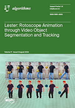
This article introduces Lester, a novel method with which to automatically synthesize retro-style 2D animations from videos. The method approaches the challenge mainly as an object segmentation and tracking problem. Video frames are processed with the Segment Anything Model (SAM), and the resulting masks are tracked through subsequent frames with DeAOT, a method for semi-supervised video object segmentation. The geometry of the masks' contours is simplified with the Douglas–Peucker algorithm. Finally, facial traits, pixelation, and a basic rim light effect can be optionally added. The results show that the method exhibits an excellent temporal consistency and can correctly process videos with different poses and appearances, dynamic shots, partial shots, and diverse backgrounds. View this paper
  • Issues are regarded as officially published after their release is announced to the table of contents alert mailing list.
  • You may sign up for e-mail alerts to receive table of contents of newly released issues.
  • PDF is the official format for papers published in both, html and pdf forms. To view the papers in pdf format, click on the "PDF Full-text" link, and use the free Adobe Reader to open them.
Order results
Result details
Section
Select all
Export citation of selected articles as:
13 pages, 4381 KiB  
Article
Extended General Malfatti’s Problem
by Ching-Shoei Chiang
Algorithms 2024, 17(8), 374; https://doi.org/10.3390/a17080374 - 22 Aug 2024
Viewed by 514
Abstract
Malfatti’s problem involves three circles (called Malfatti circles) that are tangent to each other and two sides of a triangle. In this study, our objective is to extend the problem to find 6, 10, … 1ni (n > 2) circles [...] Read more.
Malfatti’s problem involves three circles (called Malfatti circles) that are tangent to each other and two sides of a triangle. In this study, our objective is to extend the problem to find 6, 10, … 1ni (n > 2) circles inside the triangle so that the three corner circles are tangent to two sides of the triangle, the boundary circles are tangent to one side of the triangle, and four other circles (at least two of them being boundary or corner circles) and the inner circles are tangent to six other circles. We call this problem the extended general Malfatti’s problem, or the Tri(Tn) problem, where Tri means that the boundary of these circles is a triangle, and Tn is the number of circles inside the triangle. In this paper, we propose an algorithm to solve the Tri(Tn) problem. Full article
(This article belongs to the Section Algorithms for Multidisciplinary Applications)
Show Figures

Graphical abstract

Graphical abstract
Full article ">Figure 1
<p>Malfatti’s problem.</p>
Full article ">Figure 2
<p>The tangency property of the Tri(T<sub>n</sub>) problem.</p>
Full article ">Figure 3
<p>The tangency graph among circles and triangle edge. (<b>a</b>) Inside of the triangle, (<b>b</b>) With the triangle edge.</p>
Full article ">Figure 4
<p>Solution for the Tri(T<sub>1</sub>) and Tri(T<sub>2</sub>) problems. (<b>a</b>) Inscribed circle. (<b>b</b>) Malfatti circle.</p>
Full article ">Figure 5
<p>Malfatti circle for an isosceles triangle. (<b>a</b>) (<span class="html-italic">l</span>,<span class="html-italic">b</span>) = (10,12) (<b>b</b>) (<span class="html-italic">l</span>,<span class="html-italic">b</span>) = (10,8).</p>
Full article ">Figure 6
<p>The angle connecting the centers of three pairwise tangent circles.</p>
Full article ">Figure 7
<p>Angle computation for Theorem 4.</p>
Full article ">Figure 8
<p>The criterion for the enlarge/reduce radius for center circle. (<b>a</b>) SA(C) &lt; 2π (<b>b</b>) SA(C) &gt; 2π. (<b>c</b>) SA(C) = 2π.</p>
Full article ">Figure 9
<p>Angles for corner, inner, and boundary circles. (<b>a</b>) Corner circle. (<b>b</b>) Boundary circle. (<b>c</b>) Inner circle.</p>
Full article ">Figure 10
<p>The criterion for enlarging/reducing the radius of the boundary circle.</p>
Full article ">Figure 11
<p>The criterion for enlarging/reducing the radius of the corner circle.</p>
Full article ">Figure 12
<p>All circles in the triangle should also be tangent to the triangle.</p>
Full article ">Figure 13
<p>The Tri(T<sub>n</sub>) problem.</p>
Full article ">
46 pages, 501 KiB  
Article
Algorithms for Various Trigonometric Power Sums
by Victor Kowalenko
Algorithms 2024, 17(8), 373; https://doi.org/10.3390/a17080373 - 22 Aug 2024
Viewed by 620
Abstract
In this paper, algorithms for different types of trigonometric power sums are developed and presented. Although interesting in their own right, these trigonometric power sums arise during the creation of an algorithm for the four types of twisted trigonometric power sums defined in [...] Read more.
In this paper, algorithms for different types of trigonometric power sums are developed and presented. Although interesting in their own right, these trigonometric power sums arise during the creation of an algorithm for the four types of twisted trigonometric power sums defined in the introduction. The primary aim in evaluating these sums is to obtain exact results in a rational form, as opposed to standard or direct evaluation, which often results in machine-dependent decimal values that can be affected by round-off errors. Moreover, since the variable, m, appearing in the denominators of the arguments of the trigonometric functions in these sums, can remain algebraic in the algorithms/codes, one can also obtain polynomial solutions in powers of m and the variable r that appears in the cosine factor accompanying the trigonometric power. The degrees of these polynomials are found to be dependent upon v, the value of the trigonometric power in the sum, which must always be specified. Full article
(This article belongs to the Special Issue Numerical Optimization and Algorithms: 2nd Edition)
20 pages, 5263 KiB  
Article
Correlation Analysis of Railway Track Alignment and Ballast Stiffness: Comparing Frequency-Based and Machine Learning Algorithms
by Saeed Mohammadzadeh, Hamidreza Heydari, Mahdi Karimi and Araliya Mosleh
Algorithms 2024, 17(8), 372; https://doi.org/10.3390/a17080372 - 22 Aug 2024
Viewed by 630
Abstract
One of the primary challenges in the railway industry revolves around achieving a comprehensive and insightful understanding of track conditions. The geometric parameters and stiffness of railway tracks play a crucial role in condition monitoring as well as maintenance work. Hence, this study [...] Read more.
One of the primary challenges in the railway industry revolves around achieving a comprehensive and insightful understanding of track conditions. The geometric parameters and stiffness of railway tracks play a crucial role in condition monitoring as well as maintenance work. Hence, this study investigated the relationship between vertical ballast stiffness and the track longitudinal level. Initially, the ballast stiffness and track longitudinal level data were acquired through a series of experimental measurements conducted on a reference test track along the Tehran–Mashhad railway line, utilizing recording cars for geometric track and stiffness recordings. Subsequently, the correlation between the track longitudinal level and ballast stiffness was surveyed using both frequency-based techniques and machine learning (ML) algorithms. The power spectrum density (PSD) as a frequency-based technique was employed, alongside ML algorithms, including linear regression, decision trees, and random forests, for correlation mining analyses. The results showed a robust and statistically significant relationship between the vertical ballast stiffness and longitudinal levels of railway tracks. Specifically, the PSD data exhibited a considerable correlation, especially within the 1–4 rad/m wave number range. Furthermore, the data analyses conducted using ML methods indicated that the values of the root mean square error (RMSE) were about 0.05, 0.07, and 0.06 for the linear regression, decision tree, and random forest algorithms, respectively, demonstrating the adequate accuracy of ML-based approaches. Full article
(This article belongs to the Special Issue Algorithms in Data Classification (2nd Edition))
Show Figures

Figure 1

Figure 1
<p>Data acquisition along Tehran–Mashhad railway line (between Semnan and Miandareh stations).</p>
Full article ">Figure 2
<p>A view of the geometric track recording car (EM120).</p>
Full article ">Figure 3
<p>Data acquisition of track stiffness: (<b>a</b>) recording car; (<b>b</b>) laser/camera system installed to bogie frame.</p>
Full article ">Figure 4
<p>Geometric representation of track deflection measuring using laser/camera system.</p>
Full article ">Figure 5
<p>Process of correlation analyses using frequency-based and ML-based algorithms.</p>
Full article ">Figure 6
<p>Machine learning-based algorithms used in current study: (<b>a</b>) linear regression algorithm, (<b>b</b>) decision tree algorithm, and (<b>c</b>) random forest algorithm.</p>
Full article ">Figure 7
<p>Longitudinal levels collected from experimental measurements: (<b>a</b>) left rail (LLL), (<b>b</b>) right rail (LLR).</p>
Full article ">Figure 8
<p>Variation in vertical rail deflection along reference railway line.</p>
Full article ">Figure 9
<p>The calculated vertical ballast stiffness along the reference railway line.</p>
Full article ">Figure 10
<p>The PSD of vertical rail deflections (y) and longitudinal levels: (<b>a</b>) LLL, (<b>b</b>) LLR.</p>
Full article ">Figure 10 Cont.
<p>The PSD of vertical rail deflections (y) and longitudinal levels: (<b>a</b>) LLL, (<b>b</b>) LLR.</p>
Full article ">Figure 11
<p>The PSD of vertical ballast stiffness (kb) and longitudinal levels: (<b>a</b>) LLL, (<b>b</b>) LLR.</p>
Full article ">
28 pages, 1897 KiB  
Article
Bi-Objective, Dynamic, Multiprocessor Open-Shop Scheduling: A Hybrid Scatter Search–Tabu Search Approach
by Tamer F. Abdelmaguid 
Algorithms 2024, 17(8), 371; https://doi.org/10.3390/a17080371 - 21 Aug 2024
Viewed by 470
Abstract
This paper presents a novel, multi-objective scatter search algorithm (MOSS) for a bi-objective, dynamic, multiprocessor open-shop scheduling problem (Bi-DMOSP). The considered objectives are the minimization of the maximum completion time (makespan) and the minimization of the mean weighted flow time. Both are particularly [...] Read more.
This paper presents a novel, multi-objective scatter search algorithm (MOSS) for a bi-objective, dynamic, multiprocessor open-shop scheduling problem (Bi-DMOSP). The considered objectives are the minimization of the maximum completion time (makespan) and the minimization of the mean weighted flow time. Both are particularly important for improving machines’ utilization and customer satisfaction level in maintenance and healthcare diagnostic systems, in which the studied Bi-DMOSP is mostly encountered. Since the studied problem is NP-hard for both objectives, fast algorithms are needed to fulfill the requirements of real-life circumstances. Previous attempts have included the development of an exact algorithm and two metaheuristic approaches based on the non-dominated sorting genetic algorithm (NSGA-II) and the multi-objective gray wolf optimizer (MOGWO). The exact algorithm is limited to small-sized instances; meanwhile, NSGA-II was found to produce better results compared to MOGWO in both small- and large-sized test instances. The proposed MOSS in this paper attempts to provide more efficient non-dominated solutions for the studied Bi-DMOSP. This is achievable via its hybridization with a novel, bi-objective tabu search approach that utilizes a set of efficient neighborhood search functions. Parameter tuning experiments are conducted first using a subset of small-sized benchmark instances for which the optimal Pareto front solutions are known. Then, detailed computational experiments on small- and large-sized instances are conducted. Comparisons with the previously developed NSGA-II metaheuristic demonstrate the superiority of the proposed MOSS approach for small-sized instances. For large-sized instances, it proves its capability of producing competitive results for instances with low and medium density. Full article
(This article belongs to the Special Issue Scheduling: Algorithms and Real-World Applications)
Show Figures

Figure 1

Figure 1
<p>Flow chart of the proposed multi-objective scatter-search metaheuristic.</p>
Full article ">Figure 2
<p>Proposed solution representation for a sample solution of the presented sample DMOSP instance.</p>
Full article ">Figure 3
<p>Gantt chart for the generated schedule based on the solution representation shown in <a href="#algorithms-17-00371-f002" class="html-fig">Figure 2</a> for the presented sample DMOSP instance.</p>
Full article ">Figure 4
<p>Chromosomes of two sample solutions to the sample DMOSP instance presented in <a href="#sec3dot2-algorithms-17-00371" class="html-sec">Section 3.2</a>: (<b>a</b>) first solution and (<b>b</b>) second solution.</p>
Full article ">Figure 5
<p>Illustration of the minimal moves needed to convert the second solution in <a href="#algorithms-17-00371-f004" class="html-fig">Figure 4</a>b to the first solution in <a href="#algorithms-17-00371-f004" class="html-fig">Figure 4</a>a. The numbers 1 through 5 correspond to the conducted five moves.</p>
Full article ">Figure 6
<p>Solution-recombination process.</p>
Full article ">Figure 7
<p>Main effect plots from the first MOSS-tuning experiments. (<b>a</b>) Main effect plots for <math display="inline"> <semantics> <mrow> <mi mathvariant="script">H</mi> <mo>(</mo> <mi mathvariant="script">D</mi> <mo>)</mo> </mrow> </semantics> </math>. (<b>b</b>) Main effect plots for the computational time.</p>
Full article ">Figure 8
<p>Progress of average performance over computational time in the second MOSS-tuning experiments. (<b>a</b>) Mean <math display="inline"> <semantics> <mrow> <mi mathvariant="script">H</mi> <mo>(</mo> <mi mathvariant="script">D</mi> <mo>)</mo> </mrow> </semantics> </math> at different <math display="inline"> <semantics> <mrow> <mi>R</mi> <mi>e</mi> <mi>f</mi> <mi>S</mi> <mi>e</mi> <mi>t</mi> <mi>S</mi> <mi>i</mi> <mi>z</mi> <mi>e</mi> </mrow> </semantics> </math> values. (<b>b</b>) Mean <math display="inline"> <semantics> <mrow> <mi mathvariant="script">H</mi> <mo>(</mo> <mi mathvariant="script">D</mi> <mo>)</mo> </mrow> </semantics> </math> at different <math display="inline"> <semantics> <msubsup> <mi>n</mi> <mrow> <mi>m</mi> <mi>a</mi> <mi>x</mi> <mi>i</mi> <mi>t</mi> <mi>r</mi> </mrow> <mrow> <mi>T</mi> <mi>S</mi> </mrow> </msubsup> </semantics> </math> values. (<b>c</b>) Mean <math display="inline"> <semantics> <mrow> <mi>T</mi> <mi>G</mi> <mi>D</mi> <mo>(</mo> <mi mathvariant="script">D</mi> <mo>)</mo> </mrow> </semantics> </math> at different <math display="inline"> <semantics> <mrow> <mi>R</mi> <mi>e</mi> <mi>f</mi> <mi>S</mi> <mi>e</mi> <mi>t</mi> <mi>S</mi> <mi>i</mi> <mi>z</mi> <mi>e</mi> </mrow> </semantics> </math> values. (<b>d</b>) Mean <math display="inline"> <semantics> <mrow> <mi>T</mi> <mi>G</mi> <mi>D</mi> <mo>(</mo> <mi mathvariant="script">D</mi> <mo>)</mo> </mrow> </semantics> </math> at different <math display="inline"> <semantics> <msubsup> <mi>n</mi> <mrow> <mi>m</mi> <mi>a</mi> <mi>x</mi> <mi>i</mi> <mi>t</mi> <mi>r</mi> </mrow> <mrow> <mi>T</mi> <mi>S</mi> </mrow> </msubsup> </semantics> </math> values.</p>
Full article ">Figure 9
<p>Box-and-whisker plots and confidence intervals for the average difference in <math display="inline"> <semantics> <mover> <mrow> <mi>T</mi> <mi>G</mi> <mi>D</mi> </mrow> <mo>¯</mo> </mover> </semantics> </math> and <math display="inline"> <semantics> <mover> <mi mathvariant="script">H</mi> <mo>¯</mo> </mover> </semantics> </math>, based on the results of a paired <span class="html-italic">t</span>-test for the computational experiments on small-sized instances at a 95% confidence level. (<b>a</b>) Results for total gravitational distances. (<b>b</b>) Results for the percentage hypervolume deviations.</p>
Full article ">Figure 10
<p>Pareto fronts and generated non-dominated solutions of both NSGA-II and MOSS for selected small-sized instances. (<b>a</b>) DMOSP-S-7. (<b>b</b>) DMOSP-S-6. (<b>c</b>) DMOSP-S-24. (<b>d</b>) DMOSP-S-17. (<b>e</b>) DMOSP-S-4. (<b>f</b>) DMOSP-S-15.</p>
Full article ">Figure 11
<p>Main effect plots for <math display="inline"> <semantics> <mrow> <mo>Δ</mo> <mover> <mrow> <mi>H</mi> <mi>V</mi> <mo>%</mo> </mrow> <mo>¯</mo> </mover> </mrow> </semantics> </math>.</p>
Full article ">Figure 12
<p>Interaction plots for <math display="inline"> <semantics> <mrow> <mo>Δ</mo> <mover> <mrow> <mi>H</mi> <mi>V</mi> <mo>%</mo> </mrow> <mo>¯</mo> </mover> </mrow> </semantics> </math>.</p>
Full article ">
23 pages, 1362 KiB  
Article
Joint Optimization of Service Migration and Resource Allocation in Mobile Edge–Cloud Computing
by Zhenli He, Liheng Li, Ziqi Lin, Yunyun Dong, Jianglong Qin and Keqin Li
Algorithms 2024, 17(8), 370; https://doi.org/10.3390/a17080370 - 21 Aug 2024
Viewed by 700
Abstract
In the rapidly evolving domain of mobile edge–cloud computing (MECC), the proliferation of Internet of Things (IoT) devices and mobile applications poses significant challenges, particularly in dynamically managing computational demands and user mobility. Current research has partially addressed aspects of service migration and [...] Read more.
In the rapidly evolving domain of mobile edge–cloud computing (MECC), the proliferation of Internet of Things (IoT) devices and mobile applications poses significant challenges, particularly in dynamically managing computational demands and user mobility. Current research has partially addressed aspects of service migration and resource allocation, yet it often falls short in thoroughly examining the nuanced interdependencies between migration strategies and resource allocation, the consequential impacts of migration delays, and the intricacies of handling incomplete tasks during migration. This study advances the discourse by introducing a sophisticated framework optimized through a deep reinforcement learning (DRL) strategy, underpinned by a Markov decision process (MDP) that dynamically adapts service migration and resource allocation strategies. This refined approach facilitates continuous system monitoring, adept decision making, and iterative policy refinement, significantly enhancing operational efficiency and reducing response times in MECC environments. By meticulously addressing these previously overlooked complexities, our research not only fills critical gaps in the literature but also enhances the practical deployment of edge computing technologies, contributing profoundly to both theoretical insights and practical implementations in contemporary digital ecosystems. Full article
(This article belongs to the Collection Feature Papers in Algorithms for Multidisciplinary Applications)
Show Figures

Figure 1

Figure 1
<p>An example of an MECC environment.</p>
Full article ">Figure 2
<p>An example of the migration process.</p>
Full article ">Figure 3
<p>Training of A2C-based dynamic migration and resource allocation algorithm.</p>
Full article ">Figure 4
<p>The impact of the number of ESs on average response delay.</p>
Full article ">Figure 5
<p>The impact of the number of ESs on failure rate.</p>
Full article ">Figure 6
<p>The impact of the time constraint on average response delay.</p>
Full article ">Figure 7
<p>The impact of the time constraint on failure rate.</p>
Full article ">Figure 8
<p>The impact of the number of users on average response delay.</p>
Full article ">Figure 9
<p>Decision-making duration for each step.</p>
Full article ">Figure 10
<p>The impact of the number of users on failure rate.</p>
Full article ">Figure 11
<p>The impact of data size on average response delay.</p>
Full article ">Figure 12
<p>The impact of data size on average failure rate.</p>
Full article ">Figure 13
<p>The impact of network scale expansion in an environment with 40 users and 20 ESs. (<b>a</b>) Average response delay. (<b>b</b>) Average failure rate.</p>
Full article ">
16 pages, 439 KiB  
Article
On the Complexity of the Bipartite Polarization Problem: From Neutral to Highly Polarized Discussions
by Teresa Alsinet, Josep Argelich, Ramón Béjar and Santi Martínez
Algorithms 2024, 17(8), 369; https://doi.org/10.3390/a17080369 - 21 Aug 2024
Viewed by 385
Abstract
The bipartite polarization problem is an optimization problem where the goal is to find the highest polarized bipartition on a weighted and labeled graph that represents a debate developed through some social network, where nodes represent user’s opinions and edges agreement or disagreement [...] Read more.
The bipartite polarization problem is an optimization problem where the goal is to find the highest polarized bipartition on a weighted and labeled graph that represents a debate developed through some social network, where nodes represent user’s opinions and edges agreement or disagreement between users. This problem can be seen as a generalization of the maxcut problem, and in previous work, approximate solutions and exact solutions have been obtained for real instances obtained from Reddit discussions, showing that such real instances seem to be very easy to solve. In this paper, we further investigate the complexity of this problem by introducing an instance generation model where a single parameter controls the polarization of the instances in such a way that this correlates with the average complexity to solve those instances. The average complexity results we obtain are consistent with our hypothesis: the higher the polarization of the instance, the easier is to find the corresponding polarized bipartition. In view of the experimental results, it is computationally feasible to implement transparent mechanisms to monitor polarization on online discussions and to inform about solutions for creating healthier social media environments. Full article
Show Figures

Figure 1

Figure 1
<p>CPU time needed to solve the instances (<b>left plot</b>) and polarization of the solution (<b>right plot</b>) as we increase the alpha value for instances with nodes ranging from 25 to 40.</p>
Full article ">Figure 2
<p>Number of nodes of the SCIP search tree needed to solve the instances as we increase the alpha value for instances with nodes ranging from 25 to 40.</p>
Full article ">Figure 3
<p>CPU time needed to solve the instances (<b>left plot</b>) and polarization of the solution (<b>right plot</b>) as we increase the alpha value (starting from 0.4) for instances with nodes ranging from 40 to 90 and with average degree equal to 3.5.</p>
Full article ">
22 pages, 2634 KiB  
Article
Identification of Crude Distillation Unit: A Comparison between Neural Network and Koopman Operator
by Abdulrazaq Nafiu Abubakar, Mustapha Kamel Khaldi, Mujahed Aldhaifallah, Rohit Patwardhan and Hussain Salloum
Algorithms 2024, 17(8), 368; https://doi.org/10.3390/a17080368 - 21 Aug 2024
Viewed by 514
Abstract
In this paper, we aimed to identify the dynamics of a crude distillation unit (CDU) using closed-loop data with NARX−NN and the Koopman operator in both linear (KL) and bilinear (KB) forms. A comparative analysis was conducted to assess the performance of each [...] Read more.
In this paper, we aimed to identify the dynamics of a crude distillation unit (CDU) using closed-loop data with NARX−NN and the Koopman operator in both linear (KL) and bilinear (KB) forms. A comparative analysis was conducted to assess the performance of each method under different experimental conditions, such as the gain, a delay and time constant mismatch, tight constraints, nonlinearities, and poor tuning. Although NARX−NN showed good training performance with the lowest Mean Squared Error (MSE), the KB demonstrated better generalization and robustness, outperforming the other methods. The KL observed a significant decline in performance in the presence of nonlinearities in inputs, yet it remained competitive with the KB under other circumstances. The use of the bilinear form proved to be crucial, as it offered a more accurate representation of CDU dynamics, resulting in enhanced performance. Full article
Show Figures

Figure 1

Figure 1
<p>The NARX−NN model representation.</p>
Full article ">Figure 2
<p>Koopman dynamics based on an NN.</p>
Full article ">Figure 3
<p>Crude distillation unit diagram.</p>
Full article ">Figure 4
<p>Summry of MSE values on the Case 1 dataset.</p>
Full article ">Figure 5
<p>Summary of MSE values on the Case 2 dataset.</p>
Full article ">Figure 6
<p>Summary of MSE values on the Case 3 dataset.</p>
Full article ">Figure 7
<p>Summary of MSE values on the Case 4 dataset.</p>
Full article ">Figure 8
<p>Summary of MSE values on the Case 5 dataset.</p>
Full article ">Figure 9
<p>Summary of MSE values on the Case 6 dataset.</p>
Full article ">Figure 10
<p>Summary of MSE values on the Case 7 dataset.</p>
Full article ">Figure 11
<p>Summary of MSE values on the Case 8 dataset.</p>
Full article ">Figure A1
<p>Case 1—predicted vs. actual output <math display="inline"><semantics> <msub> <mi>y</mi> <mn>1</mn> </msub> </semantics></math> for each model.</p>
Full article ">Figure A2
<p>Case 1—predicted vs. actual output <math display="inline"><semantics> <msub> <mi>y</mi> <mn>2</mn> </msub> </semantics></math> for each model.</p>
Full article ">Figure A3
<p>Case 1—predicted vs. actual output <math display="inline"><semantics> <msub> <mi>y</mi> <mn>3</mn> </msub> </semantics></math> for each model.</p>
Full article ">Figure A4
<p>Case 2—predicted vs. actual output <math display="inline"><semantics> <msub> <mi>y</mi> <mn>1</mn> </msub> </semantics></math> for each model.</p>
Full article ">Figure A5
<p>Case 2—predicted vs. actual output <math display="inline"><semantics> <msub> <mi>y</mi> <mn>2</mn> </msub> </semantics></math> for each model.</p>
Full article ">Figure A6
<p>Case 2—predicted vs. actual output <math display="inline"><semantics> <msub> <mi>y</mi> <mn>3</mn> </msub> </semantics></math> for each model.</p>
Full article ">Figure A7
<p>Case 3—predicted vs. actual output <math display="inline"><semantics> <msub> <mi>y</mi> <mn>1</mn> </msub> </semantics></math> for each model.</p>
Full article ">Figure A8
<p>Case 3—predicted vs. actual output <math display="inline"><semantics> <msub> <mi>y</mi> <mn>2</mn> </msub> </semantics></math> for each model.</p>
Full article ">Figure A9
<p>Case 3—predicted vs. actual output <math display="inline"><semantics> <msub> <mi>y</mi> <mn>3</mn> </msub> </semantics></math> for each model.</p>
Full article ">Figure A10
<p>Case 4—predicted vs. actual output <math display="inline"><semantics> <msub> <mi>y</mi> <mn>1</mn> </msub> </semantics></math> for each model.</p>
Full article ">Figure A11
<p>Case 4—predicted vs. actual output <math display="inline"><semantics> <msub> <mi>y</mi> <mn>2</mn> </msub> </semantics></math> for each model.</p>
Full article ">Figure A12
<p>Case 4—predicted vs. actual output <math display="inline"><semantics> <msub> <mi>y</mi> <mn>3</mn> </msub> </semantics></math> for each model.</p>
Full article ">Figure A13
<p>Case 5—predicted vs. actual output <math display="inline"><semantics> <msub> <mi>y</mi> <mn>1</mn> </msub> </semantics></math> for each model.</p>
Full article ">Figure A14
<p>Case 5—predicted vs. actual output <math display="inline"><semantics> <msub> <mi>y</mi> <mn>2</mn> </msub> </semantics></math> for each model.</p>
Full article ">Figure A15
<p>Case 5—predicted vs. actual output <math display="inline"><semantics> <msub> <mi>y</mi> <mn>3</mn> </msub> </semantics></math> for each model.</p>
Full article ">Figure A16
<p>Case 6—predicted vs. actual output <math display="inline"><semantics> <msub> <mi>y</mi> <mn>1</mn> </msub> </semantics></math> for each model.</p>
Full article ">Figure A17
<p>Case 6—predicted vs. actual output <math display="inline"><semantics> <msub> <mi>y</mi> <mn>2</mn> </msub> </semantics></math> for each model.</p>
Full article ">Figure A18
<p>Case 6—predicted vs. actual output <math display="inline"><semantics> <msub> <mi>y</mi> <mn>3</mn> </msub> </semantics></math> for each model.</p>
Full article ">Figure A19
<p>Case 7—predicted vs. actual output <math display="inline"><semantics> <msub> <mi>y</mi> <mn>1</mn> </msub> </semantics></math> for each model.</p>
Full article ">Figure A20
<p>Case 7—predicted vs. actual output <math display="inline"><semantics> <msub> <mi>y</mi> <mn>2</mn> </msub> </semantics></math> for each model.</p>
Full article ">Figure A21
<p>Case 7—predicted vs. actual output <math display="inline"><semantics> <msub> <mi>y</mi> <mn>3</mn> </msub> </semantics></math> for each model.</p>
Full article ">Figure A22
<p>Case 8—predicted vs. actual output <math display="inline"><semantics> <msub> <mi>y</mi> <mn>1</mn> </msub> </semantics></math> for each model.</p>
Full article ">Figure A23
<p>Case 8—predicted vs. actual output <math display="inline"><semantics> <msub> <mi>y</mi> <mn>2</mn> </msub> </semantics></math> for each model.</p>
Full article ">Figure A24
<p>Case 8—predicted vs. actual output <math display="inline"><semantics> <msub> <mi>y</mi> <mn>3</mn> </msub> </semantics></math> for each model.</p>
Full article ">
16 pages, 8528 KiB  
Article
Augmented Dataset for Vision-Based Analysis of Railroad Ballast via Multi-Dimensional Data Synthesis
by Kelin Ding, Jiayi Luo, Haohang Huang, John M. Hart, Issam I. A. Qamhia and Erol Tutumluer
Algorithms 2024, 17(8), 367; https://doi.org/10.3390/a17080367 - 21 Aug 2024
Viewed by 470
Abstract
Ballast serves a vital structural function in supporting railroad tracks under continuous loading. The degradation of ballast can result in issues such as inadequate drainage, lateral instability, excessive settlement, and potential service disruptions, necessitating efficient evaluation methods to ensure safe and reliable railroad [...] Read more.
Ballast serves a vital structural function in supporting railroad tracks under continuous loading. The degradation of ballast can result in issues such as inadequate drainage, lateral instability, excessive settlement, and potential service disruptions, necessitating efficient evaluation methods to ensure safe and reliable railroad operations. The incorporation of computer vision techniques into ballast inspection processes has proven effective in enhancing accuracy and robustness. Given the data-driven nature of deep learning approaches, the efficacy of these models is intrinsically linked to the quality of the training datasets, thereby emphasizing the need for a comprehensive and meticulously annotated ballast aggregate dataset. This paper presents the development of a multi-dimensional ballast aggregate dataset, constructed using empirical data collected from field and laboratory environments, supplemented with synthetic data generated by a proprietary ballast particle generator. The dataset comprises both two-dimensional (2D) data, consisting of ballast images annotated with 2D masks for particle localization, and three-dimensional (3D) data, including heightmaps, point clouds, and 3D annotations for particle localization. The data collection process encompassed various environmental lighting conditions and degradation states, ensuring extensive coverage and diversity within the training dataset. A previously developed 2D ballast particle segmentation model was trained on this augmented dataset, demonstrating high accuracy in field ballast inspections. This comprehensive database will be utilized in subsequent research to advance 3D ballast particle segmentation and shape completion, thereby facilitating enhanced inspection protocols and the development of effective ballast maintenance methodologies. Full article
(This article belongs to the Special Issue Recent Advances in Algorithms for Computer Vision Applications)
Show Figures

Figure 1

Figure 1
<p>Components in synthetic ballast dataset. <b>Left:</b> Architecture of the synthetic ballast dataset. <b>Right:</b> Examples of various data categories within the synthetic ballast dataset [<a href="#B23-algorithms-17-00367" class="html-bibr">23</a>]. (<b>a</b>–<b>c</b>) 2D synthetic ballast images under different lighting conditions. (<b>d</b>) 3D heightmap. (<b>e</b>) Masks of ballast particles for 2D synthetic ballast images. (<b>f</b>) 3D point cloud of ballast particles. (<b>g</b>) Labels of ballast particles for 3D ballast point clouds, each 3D point is rendered in a specific color that indicate the ballast particle it belongs to. (<b>h</b>) 3D completed mesh of a ballast particles. (<b>i</b>) Ballast particle size distribution curve.</p>
Full article ">Figure 2
<p>Three-dimensional laser scanner used to scan the ballast particles and export their 3D meshes.</p>
Full article ">Figure 3
<p>Morphological characteristics of the scanned meshes of individual ballast particles. Distributions of (<b>a</b>) 3D flat and elongated ratio (FER), (<b>b</b>) 3D sphericity, and (<b>c</b>) 3D angularity index (AI) [<a href="#B23-algorithms-17-00367" class="html-bibr">23</a>].</p>
Full article ">Figure 4
<p>Generation of synthetic ballast data. (<b>a</b>) Initialize base container. The bottom of the container is 3.3 ft × 3.3 ft (1 m × 1 m), and the transparent walls of the container are 6.6 ft (2 m) in height. (<b>b</b>) Generate particles &gt;3/8 in. (9.5 mm) according to the input particle size distribution (PSD) and freely release them from random locations inside the container without overlapping under gravity. (<b>c</b>) Shake the container by periodically changing the direction of the gravity to ensure uniform mixing of the ballast particles. (<b>d</b>) Calculate the height of the fine surface according to the input PSD, then add the fine surface of the same size as the bottom of the container to the scene. (<b>e</b>) Place a camera to visualize the plan view of the ballast scene and assign random textures to the ballast particles and fine material surface. (<b>f</b>) An enlarged view of the image (<b>e</b>). (<b>g</b>) Add ballast particles in sizes of 0.1~3/8 in. (2.54~9.5 mm) on top of the fine material surface to better resemble real ballast sizes in the field. (<b>h</b>) Mix textures of the fine material and the ballast particles to mimic the appearance of field ballast particles covered with fine materials. (<b>i</b>) Add ballast particles in sizes of 0.03~0.1 in. (0.762~2.54 mm) on top of the fine material surface with a hair particle system [<a href="#B23-algorithms-17-00367" class="html-bibr">23</a>].</p>
Full article ">Figure 5
<p>Synthetic ballast particles in adaptively mixed textures with different ‘<span class="html-italic">r</span>’ values [<a href="#B23-algorithms-17-00367" class="html-bibr">23</a>].</p>
Full article ">Figure 6
<p>Examples of synthetic ballast images with: (<b>a</b>–<b>c</b>) different light conditions, (<b>d</b>–<b>f</b>) different particle size distributions, and (<b>g</b>–<b>i</b>) different textures of ballast particles and fine material surface.</p>
Full article ">Figure 7
<p>Data collected from various camera perspectives include: (<b>a</b>) color image, (<b>b</b>) 2D segmentation labels (object indices), and (<b>c</b>) depth map. Through projecting all captured data into the world coordinate system, (<b>d</b>) the ground truth point cloud and (<b>e</b>) the 3D ground truth labels (different colors indicate different ballast particles) are obtained [<a href="#B23-algorithms-17-00367" class="html-bibr">23</a>].</p>
Full article ">Figure 8
<p>Comparison between TRTR and TSTR. (<b>a</b>) Experimental flowchart. (<b>b</b>) Mean average precision (<math display="inline"><semantics> <mrow> <mi>m</mi> <mi>A</mi> <mi>P</mi> </mrow> </semantics></math>) comparison. (<b>c</b>) F1-Score for <math display="inline"><semantics> <mrow> <mi>m</mi> <mi>A</mi> <mi>P</mi> </mrow> </semantics></math> and mean average recall (<math display="inline"><semantics> <mrow> <mi>m</mi> <mi>A</mi> <mi>R</mi> </mrow> </semantics></math>) comparison [<a href="#B23-algorithms-17-00367" class="html-bibr">23</a>].</p>
Full article ">Figure 9
<p>Comparison between TRTR and TATR. (<b>a</b>) Experimental flowchart. (<b>b</b>) Mean average precision (<math display="inline"><semantics> <mrow> <mi>m</mi> <mi>A</mi> <mi>P</mi> </mrow> </semantics></math>) comparison. (<b>c</b>) F1-Score calculated from <math display="inline"><semantics> <mrow> <mi>m</mi> <mi>A</mi> <mi>P</mi> </mrow> </semantics></math> and mean average recall (<math display="inline"><semantics> <mrow> <mi>m</mi> <mi>A</mi> <mi>R</mi> </mrow> </semantics></math>) comparison [<a href="#B23-algorithms-17-00367" class="html-bibr">23</a>].</p>
Full article ">Figure 10
<p>Segmentation results on a real ballast image. (<b>a</b>) Ballast segmentation results obtained from the model trained exclusively on real ballast images and (<b>b</b>) zoom-in view. (<b>c</b>) Ballast segmentation results derived from the model trained using augmented ballast images and (<b>d</b>) zoom-in view. Different colors indicate different ballast particles detected.</p>
Full article ">
19 pages, 7973 KiB  
Article
Determining Thresholds for Optimal Adaptive Discrete Cosine Transformation
by Alexander Khanov, Anastasija Shulzhenko, Anzhelika Voroshilova, Alexander Zubarev, Timur Karimov and Shakeeb Fahmi
Algorithms 2024, 17(8), 366; https://doi.org/10.3390/a17080366 - 21 Aug 2024
Viewed by 480
Abstract
The discrete cosine transform (DCT) is widely used for image and video compression. Lossy algorithms such as JPEG, WebP, BPG and many others are based on it. Multiple modifications of DCT have been developed to improve its performance. One of them is adaptive [...] Read more.
The discrete cosine transform (DCT) is widely used for image and video compression. Lossy algorithms such as JPEG, WebP, BPG and many others are based on it. Multiple modifications of DCT have been developed to improve its performance. One of them is adaptive DCT (ADCT) designed to deal with heterogeneous image structure and it may be found, for example, in the HEVC video codec. Adaptivity means that the image is divided into an uneven grid of squares: smaller ones retain information about details better, while larger squares are efficient for homogeneous backgrounds. The practical use of adaptive DCT algorithms is complicated by the lack of optimal threshold search algorithms for image partitioning procedures. In this paper, we propose a novel method for optimal threshold search in ADCT using a metric based on tonal distribution. We define two thresholds: pm, the threshold defining solid mean coloring, and ps, defining the quadtree fragment splitting. In our algorithm, the values of these thresholds are calculated via polynomial functions of the tonal distribution of a particular image or fragment. The polynomial coefficients are determined using the dedicated optimization procedure on the dataset containing images from the specific domain, urban road scenes in our case. In the experimental part of the study, we show that ADCT allows a higher compression ratio compared to non-adaptive DCT at the same level of quality loss, up to 66% for acceptable quality. The proposed algorithm may be used directly for image compression, or as a core of video compression framework in traffic-demanding applications, such as urban video surveillance systems. Full article
(This article belongs to the Special Issue Algorithms for Image Processing and Machine Vision)
Show Figures

Figure 1

Figure 1
<p>Examples of video compression using 3D DCT, comparing the original video frame and various compression techniques, with variable-temporal-length 3D DCT implementations in the bottom row, clearly showing its superiority.</p>
Full article ">Figure 2
<p>Example of adaptive 3D DCT in a video frame, showcasing both fragmenting and replacing entire fragments with their average tones.</p>
Full article ">Figure 3
<p>Example of adaptive discrete cosine transform: (<b>a</b>) original image; (<b>b</b>) quadtree grid on the image, yellow color marks the solid color fragments; (<b>c</b>) adaptive discrete cosine transform spectrum of the image (brightened up for clarity).</p>
Full article ">Figure 4
<p>Examples of image histograms: (<b>a</b>) histogram of the original image; (<b>b</b>) histogram after increasing the brightness by 40%; (<b>c</b>) histogram after normalization, i.e., extending it to the entire 0–255 spectrum width; (<b>d</b>) histogram after multiplying the brightness by 2, resulting in a “whiteout” (overexposure).</p>
Full article ">Figure 5
<p>Example of solid color fragments: (<b>a</b>) processed image; (<b>b</b>) processed image: solid color fragments are marked with yellow; (<b>c</b>) close-ups of the sky and the road surface demonstrate little impact on the overall perception unless zoomed in.</p>
Full article ">Figure 6
<p>Image quality comparison: (<b>a</b>) the original images; (<b>b</b>) high-quality ADCT; (<b>c</b>) medium-quality ADCT; (<b>d</b>) low-quality ADCT.</p>
Full article ">Figure 7
<p>Flowchart of the optimization process; the grid is the search area; each grid cell is a pair of threshold values.</p>
Full article ">Figure 8
<p>Optimal threshold values for different original ITDV values of the images.</p>
Full article ">Figure 9
<p>Examples of the test dataset frames.</p>
Full article ">Figure 10
<p>Distribution of ITDV values through all images of the considered dataset.</p>
Full article ">Figure 11
<p>Comparison of resulting MS-SSIM and compression ratio after ADCT and non-adaptive DCT for ITDV values from 9 to 16.</p>
Full article ">Figure 12
<p>Graphical comparison of proposed ADCT with non-adaptive DCT in terms of approximated bit rate vs. MS-SSIM.</p>
Full article ">Figure 13
<p>Comparison [<a href="#B25-algorithms-17-00366" class="html-bibr">25</a>] with the existing algorithms.</p>
Full article ">Figure 14
<p>Advantage in low target quality compression of ADCT over DCT and preservation of information about vehicles in the scene: (<b>a</b>) original image; (<b>b</b>) fragmentation quadtree of ADCT and grid of DCT (yellow fragments are solid color); (<b>c</b>) resulting images (details about car positions are preserved).</p>
Full article ">Figure A1
<p>Highway footage frame test: (<b>a</b>) The original image. (<b>b</b>) High-quality ADCT and DCT. (<b>c</b>) Medium-quality ADCT and DCT. (<b>d</b>) Low-quality ADCT and DCT.</p>
Full article ">Figure A2
<p>Recorder footage frame test: (<b>a</b>) The original image. (<b>b</b>) High-quality ADCT and DCT. (<b>c</b>) Medium-quality ADCT and DCT. (<b>d</b>) Low-quality ADCT and DCT.</p>
Full article ">Figure A3
<p>Dark highway photo test: (<b>a</b>) The original image. (<b>b</b>) High-quality ADCT and DCT. (<b>c</b>) Medium-quality ADCT and DCT. (<b>d</b>) Low-quality ADCT and DCT.</p>
Full article ">Figure A4
<p>Sunny highway photo test: (<b>a</b>) The original image. (<b>b</b>) High-quality ADCT and DCT. (<b>c</b>) Medium-quality ADCT and DCT. (<b>d</b>) Low-quality ADCT and DCT.</p>
Full article ">
16 pages, 5082 KiB  
Article
An Image Processing-Based Correlation Method for Improving the Characteristics of Brillouin Frequency Shift Extraction in Distributed Fiber Optic Sensors
by Yuri Konstantinov, Anton Krivosheev and Fedor Barkov
Algorithms 2024, 17(8), 365; https://doi.org/10.3390/a17080365 - 20 Aug 2024
Viewed by 755
Abstract
This paper demonstrates how the processing of Brillouin gain spectra (BGS) by two-dimensional correlation methods improves the accuracy of Brillouin frequency shift (BFS) extraction in distributed fiber optic sensor systems based on the BOTDA/BOTDR (Brillouin optical time domain analysis/reflectometry) principles. First, the spectra [...] Read more.
This paper demonstrates how the processing of Brillouin gain spectra (BGS) by two-dimensional correlation methods improves the accuracy of Brillouin frequency shift (BFS) extraction in distributed fiber optic sensor systems based on the BOTDA/BOTDR (Brillouin optical time domain analysis/reflectometry) principles. First, the spectra corresponding to different spatial coordinates of the fiber sensor are resampled. Subsequently, the resampled spectra are aligned by the position of the maximum by shifting in frequency relative to each other. The spectra aligned by the position of the maximum are then averaged, which effectively increases the signal-to-noise ratio (SNR). Finally, the Lorentzian curve fitting (LCF) method is applied to the spectrum with improved characteristics, including a reduced scanning step and an increased SNR. Simulations and experiments have demonstrated that the method is particularly efficacious when the signal-to-noise ratio does not exceed 8 dB and the frequency scanning step is coarser than 4 MHz. This is particularly relevant when designing high-speed sensors, as well as when using non-standard laser sources, such as a self-scanning frequency laser, for distributed fiber-optic sensing. Full article
(This article belongs to the Section Algorithms for Multidisciplinary Applications)
Show Figures

Figure 1

Figure 1
<p>An example of the BOTDA/BOTDR type systems applications in monitoring the condition of a civil aircraft [<a href="#B26-algorithms-17-00365" class="html-bibr">26</a>,<a href="#B27-algorithms-17-00365" class="html-bibr">27</a>,<a href="#B28-algorithms-17-00365" class="html-bibr">28</a>].</p>
Full article ">Figure 2
<p>The principle of the proposed method.</p>
Full article ">Figure 3
<p>Algorithm for checking the efficiency of the method.</p>
Full article ">Figure 4
<p>Dependences of the BFS extraction accuracy on the number of averaged spectra for spectra with SNR = 2 dB. Individual curves correspond to different scanning steps (16, 8, 4, 2, 1, and 0.5 MHz from top to bottom). Green arrow shows gain in BFS extraction accuracy. Inset: BFS extraction accuracy gain as a function of frequency step.</p>
Full article ">Figure 5
<p>Dependence of the BFS extraction accuracy on the number of averaged spectra for spectra with SNR=11 dBm. Red arrow shows loss in BFS extraction accuracy. Inset: BFS extraction accuracy gain as a function of the scan step.</p>
Full article ">Figure 6
<p>Dependence of the gain/loss in the accuracy of determining the BFS of the presented algorithm over LCF when processing the simulated spectra.</p>
Full article ">Figure 7
<p>Dependence of the BFS extraction precision on the number of averaged spectra for spectra with SNR = 2 dBm. Green arrow shows gain in BFS extraction accuracy. Inset: BFS extraction precision gain as a function of the scan step.</p>
Full article ">Figure 8
<p><b>An</b> experimental setup for obtaining BGS includes the following components: FUT (fiber under test), DAQ (digital acquisition), and NBL (narrow bandwidth laser).</p>
Full article ">Figure 9
<p>Dependence of the BFS extraction accuracy on the number of averaged spectra for experimental data with low SNR. Green arrow shows gain in BFS extraction accuracy. Inset: dependence of the gain in BFS extraction accuracy on the scanning step.</p>
Full article ">Figure 10
<p>Dependence of the BFS extraction precision on the number of averaged spectra for experimental data with low SNR. Green arrow shows gain in BFS extraction accuracy. Inset: dependence of the gain in precision on the scanning step.</p>
Full article ">Figure 11
<p>Dependence of the BFS extraction accuracy on the number of averaged spectra for experimental data with high SNR. Green arrow shows gain in BFS extraction accuracy. Inset: dependence of the gain in BFS extraction accuracy on the scanning step.</p>
Full article ">Figure 12
<p>Dependence of the BFS extraction precision number of averaged spectra for experimental data with high SNR. Green arrow shows gain in BFS extraction accuracy. Inset: dependence of the gain in BFS extraction precision on the scanning step.</p>
Full article ">Figure 13
<p>Dependence of the gain/loss in the accuracy of determining the BFS of the presented algorithm over LCF when processing the spectra obtained in the experiment.</p>
Full article ">Figure 14
<p>Illustration of the influence of the algorithm used on the spectrum shape: (<b>a</b>)—original spectrum; (<b>b</b>)—additional spectrum; and (<b>c</b>)—the result of averaging two spectra, the inset shows a close-up of the kink.</p>
Full article ">
29 pages, 8768 KiB  
Article
HRIDM: Hybrid Residual/Inception-Based Deeper Model for Arrhythmia Detection from Large Sets of 12-Lead ECG Recordings
by Syed Atif Moqurrab, Hari Mohan Rai and Joon Yoo
Algorithms 2024, 17(8), 364; https://doi.org/10.3390/a17080364 - 19 Aug 2024
Cited by 2 | Viewed by 479
Abstract
Heart diseases such as cardiovascular and myocardial infarction are the foremost reasons of death in the world. The timely, accurate, and effective prediction of heart diseases is crucial for saving lives. Electrocardiography (ECG) is a primary non-invasive method to identify cardiac abnormalities. However, [...] Read more.
Heart diseases such as cardiovascular and myocardial infarction are the foremost reasons of death in the world. The timely, accurate, and effective prediction of heart diseases is crucial for saving lives. Electrocardiography (ECG) is a primary non-invasive method to identify cardiac abnormalities. However, manual interpretation of ECG recordings for heart disease diagnosis is a time-consuming and inaccurate process. For the accurate and efficient detection of heart diseases from the 12-lead ECG dataset, we have proposed a hybrid residual/inception-based deeper model (HRIDM). In this study, we have utilized ECG datasets from various sources, which are multi-institutional large ECG datasets. The proposed model is trained on 12-lead ECG data from over 10,000 patients. We have compared the proposed model with several state-of-the-art (SOTA) models, such as LeNet-5, AlexNet, VGG-16, ResNet-50, Inception, and LSTM, on the same training and test datasets. To show the effectiveness of the computational efficiency of the proposed model, we have only trained over 20 epochs without GPU support and we achieved an accuracy of 50.87% on the test dataset for 27 categories of heart abnormalities. We found that our proposed model outperformed the previous studies which participated in the official PhysioNet/CinC Challenge 2020 and achieved fourth place as compared with the 41 official ranking teams. The result of this study indicates that the proposed model is an implying new method for predicting heart diseases using 12-lead ECGs. Full article
Show Figures

Figure 1

Figure 1
<p>Data distribution based on signal length.</p>
Full article ">Figure 2
<p>Distribution of ECG signals across 27 diagnosis categories.</p>
Full article ">Figure 3
<p>The flowchart of the utilized preprocessing technique.</p>
Full article ">Figure 4
<p>Segmented and preprocessed 12-lead ECG signals.</p>
Full article ">Figure 5
<p>Building blocks of proposed hybrid residual/inception-based deeper model (HRIDM).</p>
Full article ">Figure 6
<p>Comparison of output responses for ReLU, Leaky ReLU, sigmoid, and tanh activation functions.</p>
Full article ">Figure 7
<p>Training history curve of LeNet-5 model on training and validation data. (<b>a</b>) Accuracy, precision, and AUC. (<b>b</b>) Loss.</p>
Full article ">Figure 8
<p>Training history curve of AlexNet model on training and validation data. (<b>a</b>) Accuracy, precision, and AUC. (<b>b</b>) Loss.</p>
Full article ">Figure 9
<p>Training history curve of VGG-16 model on training and validation data. (<b>a</b>) Accuracy, precision, and AUC. (<b>b</b>) Loss.</p>
Full article ">Figure 10
<p>Training history curve of ResNet-50 model on training and validation data. (<b>a</b>) Accuracy, precision, and AUC. (<b>b</b>) Loss.</p>
Full article ">Figure 11
<p>Training history curve of Inception Network on training and validation data. (<b>a</b>) Accuracy, precision, and AUC. (<b>b</b>) Loss.</p>
Full article ">Figure 12
<p>Training history curve of LSTM model on training and validation data. (<b>a</b>) Accuracy, precision, and AUC. (<b>b</b>) Loss.</p>
Full article ">Figure 13
<p>Training history curve of proposed model on training and validation data. (<b>a</b>) Accuracy, precision, and AUC. (<b>b</b>) Loss.</p>
Full article ">Figure 14
<p>Accuracy comparison of SOTA vs. proposed model on test dataset.</p>
Full article ">Figure 15
<p>Confusion matrix of the proposed model with SNOMED CT classes on the test dataset.</p>
Full article ">
15 pages, 7315 KiB  
Article
Computer Vision Algorithms on a Raspberry Pi 4 for Automated Depalletizing
by Danilo Greco, Majid Fasihiany, Ali Varasteh Ranjbar, Francesco Masulli, Stefano Rovetta and Alberto Cabri
Algorithms 2024, 17(8), 363; https://doi.org/10.3390/a17080363 - 18 Aug 2024
Viewed by 808
Abstract
The primary objective of a depalletizing system is to automate the process of detecting and locating specific variable-shaped objects on a pallet, allowing a robotic system to accurately unstack them. Although many solutions exist for the problem in industrial and manufacturing settings, the [...] Read more.
The primary objective of a depalletizing system is to automate the process of detecting and locating specific variable-shaped objects on a pallet, allowing a robotic system to accurately unstack them. Although many solutions exist for the problem in industrial and manufacturing settings, the application to small-scale scenarios such as retail vending machines and small warehouses has not received much attention so far. This paper presents a comparative analysis of four different computer vision algorithms for the depalletizing task, implemented on a Raspberry Pi 4, a very popular single-board computer with low computer power suitable for the IoT and edge computing. The algorithms evaluated include the following: pattern matching, scale-invariant feature transform, Oriented FAST and Rotated BRIEF, and Haar cascade classifier. Each technique is described and their implementations are outlined. Their evaluation is performed on the task of box detection and localization in the test images to assess their suitability in a depalletizing system. The performance of the algorithms is given in terms of accuracy, robustness to variability, computational speed, detection sensitivity, and resource consumption. The results reveal the strengths and limitations of each algorithm, providing valuable insights for selecting the most appropriate technique based on the specific requirements of a depalletizing system. Full article
(This article belongs to the Special Issue Recent Advances in Algorithms for Computer Vision Applications)
Show Figures

Figure 1

Figure 1
<p>Some use cases: (<b>a</b>) pellet fuel bags, (<b>b</b>) stones, (<b>c</b>) leather (image credit: Ted McGrath on Flickr, CC BY-NC-SA 2.0), (<b>d</b>) coffee bags.</p>
Full article ">Figure 2
<p>Raspberry PI 4 and camera.</p>
Full article ">Figure 3
<p>Reference setup.</p>
Full article ">Figure 4
<p>Experimental methodology.</p>
Full article ">Figure 5
<p>Pattern matching object detection technique tested on the matchboxes image.</p>
Full article ">Figure 6
<p>SIFT object detection technique tested on the matchboxes image.</p>
Full article ">Figure 7
<p>ORB object detection technique tested on the matchboxes image.</p>
Full article ">Figure 8
<p>Haar classifier object detection technique tested on the matchboxes image.</p>
Full article ">
24 pages, 4114 KiB  
Systematic Review
Utilization of Machine Learning Algorithms for the Strengthening of HIV Testing: A Systematic Review
by Musa Jaiteh, Edith Phalane, Yegnanew A. Shiferaw, Karen Alida Voet and Refilwe Nancy Phaswana-Mafuya
Algorithms 2024, 17(8), 362; https://doi.org/10.3390/a17080362 - 17 Aug 2024
Viewed by 1426
Abstract
Several machine learning (ML) techniques have demonstrated efficacy in precisely forecasting HIV risk and identifying the most eligible individuals for HIV testing in various countries. Nevertheless, there is a data gap on the utility of ML algorithms in strengthening HIV testing worldwide. This [...] Read more.
Several machine learning (ML) techniques have demonstrated efficacy in precisely forecasting HIV risk and identifying the most eligible individuals for HIV testing in various countries. Nevertheless, there is a data gap on the utility of ML algorithms in strengthening HIV testing worldwide. This systematic review aimed to evaluate how effectively ML algorithms can enhance the efficiency and accuracy of HIV testing interventions and to identify key outcomes, successes, gaps, opportunities, and limitations in their implementation. This review was guided by the Preferred Reporting Items for Systematic Reviews and Meta-Analysis guidelines. A comprehensive literature search was conducted via PubMed, Google Scholar, Web of Science, Science Direct, Scopus, and Gale OneFile databases. Out of the 845 identified articles, 51 studies were eligible. More than 75% of the articles included in this review were conducted in the Americas and various parts of Sub-Saharan Africa, and a few were from Europe, Asia, and Australia. The most common algorithms applied were logistic regression, deep learning, support vector machine, random forest, extreme gradient booster, decision tree, and the least absolute shrinkage selection operator model. The findings demonstrate that ML techniques exhibit higher accuracy in predicting HIV risk/testing compared to traditional approaches. Machine learning models enhance early prediction of HIV transmission, facilitate viable testing strategies to improve the efficiency of testing services, and optimize resource allocation, ultimately leading to improved HIV testing. This review points to the positive impact of ML in enhancing early prediction of HIV spread, optimizing HIV testing approaches, improving efficiency, and eventually enhancing the accuracy of HIV diagnosis. We strongly recommend the integration of ML into HIV testing programs for efficient and accurate HIV testing. Full article
Show Figures

Graphical abstract

Graphical abstract
Full article ">Figure 1
<p>PRISMA flow chart representing the review selection process. Note: Reviews—any form of review article; Wrong intervention/outcome—uses of ML in CD4 and viral load testing, uses of ML in other HIV prevention and treatment protocols other than HIV testing, papers without results, and papers that reported findings related to ML in relation to HIV risk, status, and testing; Wrong design—studies without an ML approach or predictive modeling comparable to that in ML; Wrong population—studies on individuals less than 15 years old.</p>
Full article ">Figure 2
<p>Distribution of studies by region. Note: Seven studies were conducted in multiple countries.</p>
Full article ">Figure 3
<p>Distribution of studies by country.</p>
Full article ">Figure 4
<p>Yearly publication of the selected studies.</p>
Full article ">Figure 5
<p>Study characteristics. PLHIV: people living with HIV; MSM: men who have sex with men.</p>
Full article ">
28 pages, 5276 KiB  
Article
Frequency-Domain and Spatial-Domain MLMVN-Based Convolutional Neural Networks
by Igor Aizenberg and Alexander Vasko
Algorithms 2024, 17(8), 361; https://doi.org/10.3390/a17080361 - 17 Aug 2024
Viewed by 638
Abstract
This paper presents a detailed analysis of a convolutional neural network based on multi-valued neurons (CNNMVN) and a fully connected multilayer neural network based on multi-valued neurons (MLMVN), employed here as a convolutional neural network in the frequency domain. We begin by providing [...] Read more.
This paper presents a detailed analysis of a convolutional neural network based on multi-valued neurons (CNNMVN) and a fully connected multilayer neural network based on multi-valued neurons (MLMVN), employed here as a convolutional neural network in the frequency domain. We begin by providing an overview of the fundamental concepts underlying CNNMVN, focusing on the organization of convolutional layers and the CNNMVN learning algorithm. The error backpropagation rule for this network is justified and presented in detail. Subsequently, we consider how MLMVN can be used as a convolutional neural network in the frequency domain. It is shown that each neuron in the first hidden layer of MLMVN may work as a frequency-domain convolutional kernel, utilizing the Convolution Theorem. Essentially, these neurons create Fourier transforms of the feature maps that would have resulted from the convolutions in the spatial domain performed in regular convolutional neural networks. Furthermore, we discuss optimization techniques for both networks and compare the resulting convolutions to explore which features they extract from images. Finally, we present experimental results showing that both approaches can achieve high accuracy in image recognition. Full article
(This article belongs to the Special Issue Machine Learning Algorithms for Image Understanding and Analysis)
Show Figures

Figure 1

Figure 1
<p>The <math display="inline"><semantics> <mrow> <msup> <mrow> <mi>i</mi> </mrow> <mrow> <mi>t</mi> <mi>h</mi> </mrow> </msup> </mrow> </semantics></math> weights of the <math display="inline"><semantics> <mrow> <mi>m</mi> <mo>+</mo> <msup> <mrow> <mn>1</mn> </mrow> <mrow> <mi>s</mi> <mi>t</mi> </mrow> </msup> </mrow> </semantics></math> layer neurons are responsible for processing the output of the <math display="inline"><semantics> <mrow> <msup> <mrow> <mi>i</mi> </mrow> <mrow> <mi>t</mi> <mi>h</mi> </mrow> </msup> </mrow> </semantics></math> neuron in the preceding <math display="inline"><semantics> <mrow> <msup> <mrow> <mi>m</mi> </mrow> <mrow> <mi>t</mi> <mi>h</mi> </mrow> </msup> </mrow> </semantics></math> layer.</p>
Full article ">Figure 2
<p>Passing the flattened feature maps to the first fully connected layer (<b>a</b>) is analogous to the same process between the fully connected layers (<b>b</b>).</p>
Full article ">Figure 3
<p>Convolution process of the <math display="inline"><semantics> <mrow> <mn>4</mn> <mo>×</mo> <mn>4</mn> </mrow> </semantics></math> image by the <math display="inline"><semantics> <mrow> <mn>2</mn> <mo>×</mo> <mn>2</mn> </mrow> </semantics></math> kernel with stride 1. White pixels determine the kernel position, and a yellow pixel is the target pixel. On picture (<b>a</b>), we see a single possible kernel position where the <math display="inline"><semantics> <mrow> <msub> <mrow> <mi>x</mi> </mrow> <mrow> <mn>11</mn> </mrow> </msub> </mrow> </semantics></math> pixel is involved into a convolution. On picture (<b>b</b>), we can see that pixel <math display="inline"><semantics> <mrow> <msub> <mrow> <mi>x</mi> </mrow> <mrow> <mn>33</mn> </mrow> </msub> </mrow> </semantics></math> is participating in the convolution four times—every time in a different kernel position.</p>
Full article ">Figure 4
<p>Backward convolution process. The blue square contains the errors of the feature map obtained in the second convolutional layer padded with zeros. The white square is the kernel rotated by <math display="inline"><semantics> <mrow> <mn>180</mn> <mo>°</mo> </mrow> </semantics></math>. The green square represents errors of the feature map in the first convolutional layer.</p>
Full article ">Figure 5
<p>Process of the Fourier coefficients pooling: (<b>a</b>) the Fourier coefficients of the image; (<b>b</b>) Fourier coefficients with circular shift; (<b>c</b>) extraction of the frequencies around DC frequency.</p>
Full article ">Figure 6
<p>CNNMVN accuracy for MNIST dataset with different normalization.</p>
Full article ">Figure 7
<p>CNNMVN accuracy for Fashion MNIST dataset with different normalization.</p>
Full article ">Figure 8
<p>MLMVN as a Frequency domain CNN accuracy for MNIST dataset using 1–5, 1–6, 1–7 frequencies and the original image as input.</p>
Full article ">Figure 9
<p>Accuracy of MLMVN as a frequency-domain CNN for Fashion MNIST dataset using 1–7, 1–8, 1–9 frequencies and the original image as input.</p>
Full article ">Figure 10
<p>Accuracy of MLMVN as a frequency-domain CNN for MNIST with strict batch learning.</p>
Full article ">Figure 11
<p>Accuracy of MLMVN as a frequency-domain CNN for Fashion MNIST with strict batch learning.</p>
Full article ">Figure 12
<p>Comparison of an original image (<b>a</b>) with the frequency-domain downsampled image (<b>d</b>), and results of spatial-domain convolutions performed by CNNMVN (<b>b</b>,<b>c</b>) compared with those of frequency-domain convolutions performed by MLMVN (<b>e</b>,<b>f</b>). Figure description: (<b>a</b>) Original image; (<b>b</b>) After convolution with the 7th kernel; (<b>c</b>) After convolution with the 26th kernel; (<b>d</b>) Original image after frequency-domain downsampling (frequencies 1–5 were used) and inverse Fourier transform; (<b>e</b>) After convolution with the 221st kernel; (<b>f</b>) After convolution with the 366th kernel.</p>
Full article ">
12 pages, 6087 KiB  
Article
Detection of Subtle ECG Changes Despite Superimposed Artifacts by Different Machine Learning Algorithms
by Matthias Noitz, Christoph Mörtl, Carl Böck, Christoph Mahringer, Ulrich Bodenhofer, Martin W. Dünser and Jens Meier
Algorithms 2024, 17(8), 360; https://doi.org/10.3390/a17080360 - 16 Aug 2024
Viewed by 492
Abstract
Analyzing electrocardiographic (ECG) signals is crucial for evaluating heart function and diagnosing cardiac pathology. Traditional methods for detecting ECG changes often rely on offline analysis or subjective visual inspection, which may overlook subtle variations, particularly in the case of artifacts. In this theoretical, [...] Read more.
Analyzing electrocardiographic (ECG) signals is crucial for evaluating heart function and diagnosing cardiac pathology. Traditional methods for detecting ECG changes often rely on offline analysis or subjective visual inspection, which may overlook subtle variations, particularly in the case of artifacts. In this theoretical, proof-of-concept study, we investigated the potential of five different machine learning algorithms [random forests (RFs), gradient boosting methods (GBMs), deep neural networks (DNNs), an ensemble learning technique, as well as logistic regression] to detect subtle changes in the morphology of synthetically generated ECG beats despite artifacts. Following the generation of a synthetic ECG beat using the standardized McSharry algorithm, the baseline ECG signal was modified by changing the amplitude of different ECG components by 0.01–0.06 mV. In addition, a Gaussian jitter of 0.1–0.3 mV was overlaid to simulate artifacts. Five different machine learning algorithms were then applied to detect differences between the modified ECG beats. The highest discriminatory potency, as assessed by the discriminatory accuracy, was achieved by RFs and GBMs (accuracy of up to 1.0), whereas the least accurate results were obtained by logistic regression (accuracy approximately 10% less). In a second step, a feature importance algorithm (Boruta) was used to discriminate which signal parts were responsible for difference detection. For all comparisons, only signal components that had been modified in advance were used for discretion, demonstrating that the RF model focused on the appropriate signal elements. Our findings highlight the potential of RFs and GBMs as valuable tools for detecting subtle ECG changes despite artifacts, with implications for enhancing clinical diagnosis and monitoring. Further studies are needed to validate our findings with clinical data. Full article
(This article belongs to the Special Issue Machine Learning in Medical Signal and Image Processing (2nd Edition))
Show Figures

Figure 1

Figure 1
<p>Synthetic physiologic baseline ECG trace generated using standardized McSharry algorithm. mV, millivolt; ms, millisecond; P, P wave (depolarization atria); QRS, Q, R, S waves (depolarization ventricles); T, T wave (repolarization ventricles).</p>
Full article ">Figure 2
<p>Accuracies of machine learning algorithms in difference detection of ECG patterns using three increasing identical Gaussian jitters (0.1 mV, 0.2 mV, 0.3 mV). ACC, accuracy; mV, millivolt.</p>
Full article ">Figure 3
<p>Comparison of feature importances (indicated by dense, black area under the curve) in ECG pattern differentiation using Boruta feature selection algorithm. P, Q, R, S, and T waves at a fixed difference from baseline ECG of 0.06 mV are depicted, corresponding to a sequentially increased Gaussian jitter (0.1 mV, 0.2 mV, 0.3 mV). Red curve represents the synthetic baseline ECG trace modified by the superimposed Gaussian jitter imitating artifacts. X-axis depicts time of ECG intervals in ms, and y-axis depicts amplitude of ECG signal in mV. ms, milliseconds; mV, millivolt; Δ, respective change from baseline ECG trace; P, P wave (depolarization atria); QRS, Q, R, S waves (depolarization ventricles); T, T wave (repolarization ventricles).</p>
Full article ">Figure 4
<p>Accuracy heat maps of different machine learning algorithms in difference detection of ECG patterns displaying ST segment depression (<b>A</b>) and Long-QT syndrome (<b>B</b>) using three increasing identical Gaussian jitter values (0.1 mV, 0.2 mV, 0.3 mV). ACC, accuracy; DNN, deep neural network; EL, ensemble learning method; GBM, gradient boosting machine; LR, logistic regression; mV, millivolt; RF, random forest.</p>
Full article ">Figure 5
<p>Feature importances (indicated by dense, black area under the curve) in ECG pattern differentiation using Boruta feature selection algorithm. Red curve represents the synthetic baseline ECG trace (<b>left</b>; ST segment depression; <b>right</b>: Long-QT syndrome) modified by the sequentially increased superimposed Gaussian jitter imitating artifacts (0.1 mV, 0.2 mV, 0.3 mV). X-axis depicts time of ECG intervals in ms, and y-axis depicts amplitude of ECG signal in mV. ms, milliseconds; mV, millivolt; P, P wave (depolarization atria); QRS, Q, R, S waves (depolarization ventricles); T, T wave (repolarization ventricles).</p>
Full article ">
21 pages, 347 KiB  
Article
Exploring Clique Transversal Variants on Distance-Hereditary Graphs: Computational Insights and Algorithmic Approaches
by Chuan-Min Lee
Algorithms 2024, 17(8), 359; https://doi.org/10.3390/a17080359 - 16 Aug 2024
Viewed by 570
Abstract
The clique transversal problem is a critical concept in graph theory, focused on identifying a minimum subset of vertices that intersects all maximal cliques in a graph. This problem and its variations—such as the k-fold clique, {k}-clique, minus clique, [...] Read more.
The clique transversal problem is a critical concept in graph theory, focused on identifying a minimum subset of vertices that intersects all maximal cliques in a graph. This problem and its variations—such as the k-fold clique, {k}-clique, minus clique, and signed clique transversal problems—have received significant interest due to their theoretical importance and practical applications. This paper examines the k-fold clique, {k}-clique, minus clique, and signed clique transversal problems on distance-hereditary graphs. Known for their distinctive structural properties, distance hereditary graphs provide an ideal framework for studying these problem variants. By exploring these issues in the context of distance-hereditary graphs, this research enhances the understanding of the computational challenges and the potential for developing efficient algorithms to address these problems. Full article
Show Figures

Figure 1

Figure 1
<p>(<b>a</b>) A distance-hereditary graph <span class="html-italic">G</span>. (<b>b</b>) A <math display="inline"><semantics> <mrow> <mi>P</mi> <mi>T</mi> <mi>F</mi> </mrow> </semantics></math>-tree of <span class="html-italic">G</span>.</p>
Full article ">
21 pages, 3425 KiB  
Article
Directed Clustering of Multivariate Data Based on Linear or Quadratic Latent Variable Models
by Yingjuan Zhang and Jochen Einbeck
Algorithms 2024, 17(8), 358; https://doi.org/10.3390/a17080358 - 16 Aug 2024
Viewed by 593
Abstract
We consider situations in which the clustering of some multivariate data is desired, which establishes an ordering of the clusters with respect to an underlying latent variable. As our motivating example for a situation where such a technique is desirable, we consider scatterplots [...] Read more.
We consider situations in which the clustering of some multivariate data is desired, which establishes an ordering of the clusters with respect to an underlying latent variable. As our motivating example for a situation where such a technique is desirable, we consider scatterplots of traffic flow and speed, where a pattern of consecutive clusters can be thought to be linked by a latent variable, which is interpretable as traffic density. We focus on latent structures of linear or quadratic shapes, and present an estimation methodology based on expectation–maximization, which estimates both the latent subspace and the clusters along it. The directed clustering approach is summarized in two algorithms and applied to the traffic example outlined. Connections to related methodology, including principal curves, are briefly drawn. Full article
(This article belongs to the Special Issue Supervised and Unsupervised Classification Algorithms (2nd Edition))
Show Figures

Figure 1

Figure 1
<p>Speed-flow data on a California freeway with K-means clustering. The cluster centers are marked with + symbols. <b>Left</b>: Traditional shape of the ‘Fundamental diagram’, recorded from 9 July 2007 9:00 to 10 July 2007 21:59 by VDS detector 1202263 on California Freeway SR57-N. <b>Right</b>: An unusual pattern involving traffic by heavy vehicles on a slow lane, recorded on 9 July 2007 from 0:00 to 19:59 by VDS detector 1213624 on freeway SR57-S. Each point in the plots corresponds to the number of vehicles and average speed over 5-min intervals.</p>
Full article ">Figure 2
<p>Simulated data with a sample size of 500. The fitted curve is displayed in black, and the mixture centres are given by red triangles.</p>
Full article ">Figure 3
<p>Estimations of parameters <math display="inline"><semantics> <mrow> <mi>π</mi> <mo>=</mo> <msup> <mrow> <mo>(</mo> <msub> <mi>π</mi> <mn>1</mn> </msub> <mo>,</mo> <msub> <mi>π</mi> <mn>2</mn> </msub> <mo>,</mo> <msub> <mi>π</mi> <mn>3</mn> </msub> <mo>,</mo> <msub> <mi>π</mi> <mn>4</mn> </msub> <mo>)</mo> </mrow> <mi>T</mi> </msup> </mrow> </semantics></math> with different sample sizes.</p>
Full article ">Figure 4
<p>Estimations of parameters <math display="inline"><semantics> <mrow> <msub> <mi>z</mi> <mi>k</mi> </msub> <mo>=</mo> <msup> <mrow> <mo>(</mo> <msub> <mi>z</mi> <mn>1</mn> </msub> <mo>,</mo> <msub> <mi>z</mi> <mn>2</mn> </msub> <mo>,</mo> <msub> <mi>z</mi> <mn>3</mn> </msub> <mo>,</mo> <msub> <mi>z</mi> <mn>4</mn> </msub> <mo>)</mo> </mrow> <mi>T</mi> </msup> </mrow> </semantics></math> with different sample sizes.</p>
Full article ">Figure 5
<p>Estimations of parameters <math display="inline"><semantics> <mrow> <mi>β</mi> <mo>=</mo> <msup> <mrow> <mo>(</mo> <msub> <mi>β</mi> <mn>1</mn> </msub> <mo>,</mo> <msub> <mi>β</mi> <mn>2</mn> </msub> <mo>)</mo> </mrow> <mi>T</mi> </msup> </mrow> </semantics></math> with different sample sizes.</p>
Full article ">Figure 6
<p>Estimations of parameters <math display="inline"><semantics> <mrow> <mi>η</mi> <mo>=</mo> <msup> <mrow> <mo>(</mo> <msub> <mi>η</mi> <mn>1</mn> </msub> <mo>,</mo> <msub> <mi>η</mi> <mn>2</mn> </msub> <mo>)</mo> </mrow> <mi>T</mi> </msup> </mrow> </semantics></math> with different sample sizes.</p>
Full article ">Figure 7
<p>The <tt>calspeedflow</tt> data from the northbound freeway SR57-N, fitted with a quadratic curve (in blue) and mass points represented by red triangles, with different numbers of mixture components.</p>
Full article ">Figure 8
<p>Speed-flow data from the southbound freeway SR57-S, fitted with a quadratic curve (in blue), and mass points represented by red triangles, with different numbers of mixture components.</p>
Full article ">Figure 9
<p>For the <tt>calspeedflow data</tt>, <b>left panel</b>: clustering of the speed-flow data using the MAP rule; <b>right panel</b>: clustered projections (dashed lines) of the the speed-flow data.</p>
Full article ">Figure 10
<p>For the second speed-flow dataset, on the southbound freeway SR57-S, <b>left panel</b>: clustering of the speed-flow data using the MAP rule; <b>right panel</b>: clustered projections (dashed lines) of the speed-flow data.</p>
Full article ">Figure 11
<p>The ratio of flow over speed against <math display="inline"><semantics> <msub> <mi>z</mi> <mi>k</mi> </msub> </semantics></math> for the two speed-flow datasets, presented in the same order as in <a href="#algorithms-17-00358-f001" class="html-fig">Figure 1</a>.</p>
Full article ">Figure 12
<p><b>Top</b>: Hastie–Stuetzle (<b>left</b>, solid) and local principal curve (<b>right</b>, solid) with orthogonal projections (dashed) of the data onto the fitted curve; <b>bottom</b>: the fitted curve (solid) resulting from the quadratic latent variable model, with projections (dashed) onto the curve defined by the realization of the latent variable at the posterior random effect of the respective data point.</p>
Full article ">Figure A1
<p>The clustering of <tt>calspeedflow</tt> data using the variance parametrization with different diagonal matrices for different mixture components for <math display="inline"><semantics> <mrow> <mi>K</mi> <mo>=</mo> <mn>4</mn> </mrow> </semantics></math> and <math display="inline"><semantics> <mrow> <mi>K</mi> <mo>=</mo> <mn>5</mn> </mrow> </semantics></math>.</p>
Full article ">
24 pages, 4557 KiB  
Article
A System Design Perspective for Business Growth in a Crowdsourced Data Labeling Practice
by Vahid Hajipour, Sajjad Jalali, Francisco Javier Santos-Arteaga, Samira Vazifeh Noshafagh and Debora Di Caprio
Algorithms 2024, 17(8), 357; https://doi.org/10.3390/a17080357 - 15 Aug 2024
Viewed by 394
Abstract
Data labeling systems are designed to facilitate the training and validation of machine learning algorithms under the umbrella of crowdsourcing practices. The current paper presents a novel approach for designing a customized data labeling system, emphasizing two key aspects: an innovative payment mechanism [...] Read more.
Data labeling systems are designed to facilitate the training and validation of machine learning algorithms under the umbrella of crowdsourcing practices. The current paper presents a novel approach for designing a customized data labeling system, emphasizing two key aspects: an innovative payment mechanism for users and an efficient configuration of output results. The main problem addressed is the labeling of datasets where golden items are utilized to verify user performance and assure the quality of the annotated outputs. Our proposed payment mechanism is enhanced through a modified skip-based golden-oriented function that balances user penalties and prevents spam activities. Additionally, we introduce a comprehensive reporting framework to measure aggregated results and accuracy levels, ensuring the reliability of the labeling output. Our findings indicate that the proposed solutions are pivotal in incentivizing user participation, thereby reinforcing the applicability and profitability of newly launched labeling systems. Full article
(This article belongs to the Collection Feature Papers in Algorithms)
Show Figures

Figure 1

Figure 1
<p>General process of a data labeling system.</p>
Full article ">Figure 2
<p>True (✓)/False (×)-type labeling questions. (<b>a</b>) Considering positive golden items. (<b>b</b>) Considering both positive and negative golden items.</p>
Full article ">Figure 3
<p>Sensitivity analysis of the shape parameter (<span class="html-italic">T</span>) absent incorrect labeling of golden items.</p>
Full article ">Figure 4
<p>Sensitivity analysis of the shape parameter (<span class="html-italic">T</span>) without skipping any golden item.</p>
Full article ">
33 pages, 14331 KiB  
Article
A Virtual Machine Platform Providing Machine Learning as a Programmable and Distributed Service for IoT and Edge On-Device Computing: Architecture, Transformation, and Evaluation of Integer Discretization
by Stefan Bosse
Algorithms 2024, 17(8), 356; https://doi.org/10.3390/a17080356 - 15 Aug 2024
Viewed by 620
Abstract
Data-driven models used for predictive classification and regression tasks are commonly computed using floating-point arithmetic and powerful computers. We address constraints in distributed sensor networks like the IoT, edge, and material-integrated computing, providing only low-resource embedded computers with sensor data that are acquired [...] Read more.
Data-driven models used for predictive classification and regression tasks are commonly computed using floating-point arithmetic and powerful computers. We address constraints in distributed sensor networks like the IoT, edge, and material-integrated computing, providing only low-resource embedded computers with sensor data that are acquired and processed locally. Sensor networks are characterized by strong heterogeneous systems. This work introduces and evaluates a virtual machine architecture that provides ML as a service layer (MLaaS) on the node level and addresses very low-resource distributed embedded computers (with less than 20 kB of RAM). The VM provides a unified ML instruction set architecture that can be programmed to implement decision trees, ANN, and CNN model architectures using scaled integer arithmetic only. Models are trained primarily offline using floating-point arithmetic, finally converted by an iterative scaling and transformation process, demonstrated in this work by two tests based on simulated and synthetic data. This paper is an extended version of the FedCSIS 2023 conference paper providing new algorithms and ML applications, including ANN/CNN-based regression and classification tasks studying the effects of discretization on classification and regression accuracy. Full article
(This article belongs to the Special Issue Algorithms for Network Systems and Applications)
Show Figures

Figure 1

Figure 1
<p>ARM Cortex M0-based sensor node (STM32L031) implementing the REXA VM for material-integrated GUW sensing with NFC for energy transfer and bidirectional communication with only 8 kB of RAM and 32 kB of ROM.</p>
Full article ">Figure 2
<p>Principle REXA VM network architecture using different wired and wireless communication technologies.</p>
Full article ">Figure 3
<p>Basic REXA-VM architecture with integrated JIT compiler, stacks, and byte-code processor [<a href="#B11-algorithms-17-00356" class="html-bibr">11</a>,<a href="#B12-algorithms-17-00356" class="html-bibr">12</a>].</p>
Full article ">Figure 4
<p>(<b>Left</b>) Incremental growing code segment (single-tasking), persistent code cannot be removed. (<b>Right</b>) Dynamically partitioned code segments using code frames and linking code frames due to fragmentation.</p>
Full article ">Figure 5
<p>Exploding output values for negative x-values (<span class="html-italic">e</span><sup>−x</sup> term) and positive x-values (<span class="html-italic">e</span><sup>x</sup> term) of the exponential function.</p>
Full article ">Figure 6
<p>Relative discretization error of integer-scaled LUT-based approximation of the <span class="html-italic">log10</span> function for different Δ<span class="html-italic">x</span> values (1,2,4) and LUT sizes of 90, 45, and 23, respectively.</p>
Full article ">Figure 7
<p>Relative discretization error of integer-scaled LUT-interpolated approximation of the <span class="html-italic">sigmoid</span> function using the discretized <span class="html-italic">log10</span> LUT-interpolation function for different LUT resolutions and sigmoid segment ranges <span class="html-italic">R</span>. The small error plots show only positive x values.</p>
Full article ">Figure 8
<p>Relative discretization error of integer-scaled LUT-interpolated approximation of the <span class="html-italic">tanh</span> function using the discretized <span class="html-italic">log10</span> LUT-interpolation function.</p>
Full article ">Figure 9
<p>Phase 1 transformation (CNN). (<b>Top</b>) Transformation of 3-dim tensors into multiple vectors for convolutional and pooling layers and flattening of multiple vectors from last convolutional or pooling layer into one vector for the input of a fully connected neuronal layer. (<b>Bottom</b>) Convolutional and pooling operations factorized into sequential and accumulated vector operations.</p>
Full article ">Figure 10
<p>Scaling architectures for (<b>Top</b>) functional nodes, i.e., neurons; (<b>Bottom</b>) convolution or pooling operation.</p>
Full article ">Figure 11
<p>Accumulative scaled convolution or multi-vector input (flattening) neural network operation based on a product–sum calculation. Each accumulative iteration uses a different input scaling <span class="html-italic">s</span><sub>d</sub> normalization with respect to the output scaling <span class="html-italic">s</span>.</p>
Full article ">Figure 12
<p>The ML model transformation pipeline creating an intermediate USM and then creating a sequence of MLISA vector operations.</p>
Full article ">Figure 13
<p>GUW signal simulation using a 2 dim viscoelastic wave propagation model. (<b>Left</b>) Simulation set-up. (<b>Right</b>) Some example signals with and without damage (blue areas show damage features).</p>
Full article ">Figure 14
<p>Down-sampled GUW signal from simulation and low-pass-filtered rectified (envelope approximation) signal as input for the CNN (damage at position x = 100, y = 100).</p>
Full article ">Figure 15
<p>Foo/FooFP model analysis of the GUW regression CNN model. The classification error was always zero.</p>
Full article ">Figure 16
<p>(<b>Top</b>) Analysis of the ANN FP and DS models comparing RMSE and E<sub>max</sub> values for different configurations of the activation function approximation, including an FPU replacement. (<b>Bottom</b>) Selected prediction results are shown with discontinuities in the top plot using ActDS configuration 5 and without using the FPU replacement for the tanh function.</p>
Full article ">
19 pages, 322 KiB  
Article
Multi-Objective Unsupervised Feature Selection and Cluster Based on Symbiotic Organism Search
by Abbas Fadhil Jasim AL-Gburi, Mohd Zakree Ahmad Nazri, Mohd Ridzwan Bin Yaakub and Zaid Abdi Alkareem Alyasseri
Algorithms 2024, 17(8), 355; https://doi.org/10.3390/a17080355 - 14 Aug 2024
Viewed by 547
Abstract
Unsupervised learning is a type of machine learning that learns from data without human supervision. Unsupervised feature selection (UFS) is crucial in data analytics, which plays a vital role in enhancing the quality of results and reducing computational complexity in huge feature spaces. [...] Read more.
Unsupervised learning is a type of machine learning that learns from data without human supervision. Unsupervised feature selection (UFS) is crucial in data analytics, which plays a vital role in enhancing the quality of results and reducing computational complexity in huge feature spaces. The UFS problem has been addressed in several research efforts. Recent studies have witnessed a surge in innovative techniques like nature-inspired algorithms for clustering and UFS problems. However, very few studies consider the UFS problem as a multi-objective problem to find the optimal trade-off between the number of selected features and model accuracy. This paper proposes a multi-objective symbiotic organism search algorithm for unsupervised feature selection (SOSUFS) and a symbiotic organism search-based clustering (SOSC) algorithm to generate the optimal feature subset for more accurate clustering. The efficiency and robustness of the proposed algorithm are investigated on benchmark datasets. The SOSUFS method, combined with SOSC, demonstrated the highest f-measure, whereas the KHCluster method resulted in the lowest f-measure. SOSFS effectively reduced the number of features by more than half. The proposed symbiotic organisms search-based optimal unsupervised feature-selection (SOSUFS) method, along with search-based optimal clustering (SOSC), was identified as the top-performing clustering approach. Following this, the SOSUFS method demonstrated strong performance. In summary, this empirical study indicates that the proposed algorithm significantly surpasses state-of-the-art algorithms in both efficiency and effectiveness. Unsupervised learning in artificial intelligence involves machine-learning techniques that learn from data without human supervision. Unlike supervised learning, unsupervised machine-learning models work with unlabeled data to uncover patterns and insights independently, without explicit guidance or instruction. Full article
20 pages, 6532 KiB  
Article
Machine Learning Analysis Using the Black Oil Model and Parallel Algorithms in Oil Recovery Forecasting
by Bazargul Matkerim, Aksultan Mukhanbet, Nurislam Kassymbek, Beimbet Daribayev, Maksat Mustafin and Timur Imankulov
Algorithms 2024, 17(8), 354; https://doi.org/10.3390/a17080354 - 14 Aug 2024
Viewed by 664
Abstract
The accurate forecasting of oil recovery factors is crucial for the effective management and optimization of oil production processes. This study explores the application of machine learning methods, specifically focusing on parallel algorithms, to enhance traditional reservoir simulation frameworks using black oil models. [...] Read more.
The accurate forecasting of oil recovery factors is crucial for the effective management and optimization of oil production processes. This study explores the application of machine learning methods, specifically focusing on parallel algorithms, to enhance traditional reservoir simulation frameworks using black oil models. This research involves four main steps: collecting a synthetic dataset, preprocessing it, modeling and predicting the oil recovery factors with various machine learning techniques, and evaluating the model’s performance. The analysis was carried out on a synthetic dataset containing parameters such as porosity, pressure, and the viscosity of oil and gas. By utilizing parallel computing, particularly GPUs, this study demonstrates significant improvements in processing efficiency and prediction accuracy. While maintaining the value of the R2 metric in the range of 0.97, using data parallelism sped up the learning process by, at best, 10.54 times. Neural network training was accelerated almost 8 times when running on a GPU. These findings underscore the potential of parallel machine learning algorithms to revolutionize the decision-making processes in reservoir management, offering faster and more precise predictive tools. This work not only contributes to computational sciences and reservoir engineering but also opens new avenues for the integration of advanced machine learning and parallel computing methods in optimizing oil recovery. Full article
Show Figures

Figure 1

Figure 1
<p>Flowchart for predicting oil recovery factor using machine learning.</p>
Full article ">Figure 2
<p>Correlation matrix.</p>
Full article ">Figure 3
<p>Dataset before adding noise.</p>
Full article ">Figure 4
<p>Dataset after adding noise.</p>
Full article ">Figure 5
<p>Stacking regressor architecture.</p>
Full article ">Figure 6
<p>Neural network architecture for the black oil model.</p>
Full article ">Figure 7
<p>Data parallelism scheme.</p>
Full article ">Figure 8
<p>Parallelism on GPU.</p>
Full article ">Figure 9
<p>Comparison of predicted versus actual values on training set.</p>
Full article ">Figure 10
<p>Comparison of predicted versus actual values on testing set.</p>
Full article ">Figure 11
<p><math display="inline"> <semantics> <mrow> <msup> <mrow> <mi>R</mi> </mrow> <mrow> <mn>2</mn> </mrow> </msup> </mrow> </semantics> </math> score of different algorithms on training set and test set.</p>
Full article ">Figure 12
<p>MSE of different algorithms on training set and test set.</p>
Full article ">Figure 13
<p>Actual vs. predicted for all models.</p>
Full article ">Figure 14
<p>SHAP visualization for linear regression (<b>left</b>) and decision tree (<b>right</b>).</p>
Full article ">
19 pages, 1604 KiB  
Article
An Efficient AdaBoost Algorithm for Enhancing Skin Cancer Detection and Classification
by Seham Gamil, Feng Zeng, Moath Alrifaey, Muhammad Asim and Naveed Ahmad
Algorithms 2024, 17(8), 353; https://doi.org/10.3390/a17080353 - 12 Aug 2024
Viewed by 1206
Abstract
Skin cancer is a prevalent and perilous form of cancer and presents significant diagnostic challenges due to its high costs, dependence on medical experts, and time-consuming procedures. The existing diagnostic process is inefficient and expensive, requiring extensive medical expertise and time. To tackle [...] Read more.
Skin cancer is a prevalent and perilous form of cancer and presents significant diagnostic challenges due to its high costs, dependence on medical experts, and time-consuming procedures. The existing diagnostic process is inefficient and expensive, requiring extensive medical expertise and time. To tackle these issues, researchers have explored the application of artificial intelligence (AI) tools, particularly machine learning techniques such as shallow and deep learning, to enhance the diagnostic process for skin cancer. These tools employ computer algorithms and deep neural networks to identify and categorize skin cancer. However, accurately distinguishing between skin cancer and benign tumors remains challenging, necessitating the extraction of pertinent features from image data for classification. This study addresses these challenges by employing Principal Component Analysis (PCA), a dimensionality-reduction approach, to extract relevant features from skin images. Additionally, accurately classifying skin images into malignant and benign categories presents another obstacle. To improve accuracy, the AdaBoost algorithm is utilized, which amalgamates weak classification models into a robust classifier with high accuracy. This research introduces a novel approach to skin cancer diagnosis by integrating Principal Component Analysis (PCA), AdaBoost, and EfficientNet B0, leveraging artificial intelligence (AI) tools. The novelty lies in the combination of these techniques to develop a robust and accurate system for skin cancer classification. The advantage of this approach is its ability to significantly reduce costs, minimize reliance on medical experts, and expedite the diagnostic process. The developed model achieved an accuracy of 93.00% using the DermIS dataset and demonstrated excellent precision, recall, and F1-score values, confirming its ability to correctly classify skin lesions as malignant or benign. Additionally, the model achieved an accuracy of 91.00% using the ISIC dataset, which is widely recognized for its comprehensive collection of annotated dermoscopic images, providing a robust foundation for training and validation. These advancements have the potential to significantly enhance the efficiency and accuracy of skin cancer diagnosis and classification. Ultimately, the integration of AI tools and techniques in skin cancer diagnosis can lead to cost reduction and improved patient outcomes, benefiting both patients and healthcare providers. Full article
Show Figures

Figure 1

Figure 1
<p>Our proposed model.</p>
Full article ">Figure 2
<p>Images of a skin lesion. (<b>a</b>) Melanoma image. (<b>b</b>) Benign image.</p>
Full article ">Figure 3
<p>Visualization of the performance metrics for algorithms classifiers.</p>
Full article ">Figure 4
<p>Visualization of the performance metrics for algorithms classifiers.</p>
Full article ">
26 pages, 501 KiB  
Article
In-Depth Analysis of GAF-Net: Comparative Fusion Approaches in Video-Based Person Re-Identification
by Moncef Boujou, Rabah Iguernaissi, Lionel Nicod, Djamal Merad and Séverine Dubuisson
Algorithms 2024, 17(8), 352; https://doi.org/10.3390/a17080352 - 11 Aug 2024
Viewed by 997
Abstract
This study provides an in-depth analysis of GAF-Net, a novel model for video-based person re-identification (Re-ID) that matches individuals across different video sequences. GAF-Net combines appearance-based features with gait-based features derived from skeletal data, offering a new approach that diverges from traditional silhouette-based [...] Read more.
This study provides an in-depth analysis of GAF-Net, a novel model for video-based person re-identification (Re-ID) that matches individuals across different video sequences. GAF-Net combines appearance-based features with gait-based features derived from skeletal data, offering a new approach that diverges from traditional silhouette-based methods. We thoroughly examine each module of GAF-Net and explore various fusion methods at the both score and feature levels, extending beyond initial simple concatenation. Comprehensive evaluations on the iLIDS-VID and MARS datasets demonstrate GAF-Net’s effectiveness across scenarios. GAF-Net achieves state-of-the-art 93.2% rank-1 accuracy on iLIDS-VID’s long sequences, while MARS results (86.09% mAP, 89.78% rank-1) reveal challenges with shorter, variable sequences in complex real-world settings. We demonstrate that integrating skeleton-based gait features consistently improves Re-ID performance, particularly with long, more informative sequences. This research provides crucial insights into multi-modal feature integration in Re-ID tasks, laying a foundation for the advancement of multi-modal biometric systems for diverse computer vision applications. Full article
(This article belongs to the Special Issue Machine Learning Algorithms for Image Understanding and Analysis)
Show Figures

Figure 1

Figure 1
<p>A schematic representation of Improved GAF-Net illustrating its three main modules, namely the appearance feature module (with various backbones), the gait feature module, and the fusion module.</p>
Full article ">Figure 2
<p>Impact of the fusion factor (<math display="inline"><semantics> <mi>λ</mi> </semantics></math>; varying from 0 to 1) on the rank-1 accuracy.</p>
Full article ">Figure 3
<p>Impact of the fusion factor value (<math display="inline"><semantics> <mi>α</mi> </semantics></math>; varying from 0 to 1) on the rank-1 accuracy.</p>
Full article ">
22 pages, 8170 KiB  
Article
Multi-Objective Resource-Constrained Scheduling in Large and Repetitive Construction Projects
by Vasiliki Lazari, Athanasios Chassiakos and Stylianos Karatzas
Algorithms 2024, 17(8), 351; https://doi.org/10.3390/a17080351 - 10 Aug 2024
Viewed by 1016
Abstract
Effective resource management constitutes a cornerstone of construction project success. This is a challenging combinatorial optimization problem with multiple and contradictory objectives whose complexity rises disproportionally with the project size and special characteristics (e.g., repetitive projects). While relevant work exists, there is still [...] Read more.
Effective resource management constitutes a cornerstone of construction project success. This is a challenging combinatorial optimization problem with multiple and contradictory objectives whose complexity rises disproportionally with the project size and special characteristics (e.g., repetitive projects). While relevant work exists, there is still a need for thorough modeling of the practical implications of non-optimal decisions. This study proposes a multi-objective model, which can realistically represent the actual loss from not meeting the resource utilization priorities and constraints of a given project, including parameters that assess the cost of exceeding the daily resource availability, the cost of moving resources in and out of the worksite, and the cost of delaying the project completion. Optimization is performed using Genetic Algorithms, with problem setups organized in a spreadsheet format for enhanced readability and the solving is conducted via commercial software. A case study consisting of 16 repetitive projects, totaling 160 activities, tested under different objective and constraint scenarios is used to evaluate the algorithm effectiveness in different project management priorities. The main study conclusions emphasize the importance of conducting multiple analyses for effective decision-making, the increasing necessity for formal optimization as a project’s size and complexity increase, and the significant support that formal optimization provides in customizing resource allocation decisions in construction projects. Full article
Show Figures

Figure 1

Figure 1
<p>Algorithm implementation flowchart.</p>
Full article ">Figure 2
<p>Network diagram structure of the examined project.</p>
Full article ">Figure 3
<p>Network diagram of the basic project.</p>
Full article ">Figure 4
<p>Resource histogram for the early start project schedule.</p>
Full article ">Figure 5
<p>Typical optimized resource allocation diagram. The red line indicates the daily resource availability.</p>
Full article ">Figure 6
<p>Resource histogram for STD criterion. The red line indicates the daily resource availability.</p>
Full article ">Figure 7
<p>Resource histogram for RLE criterion. The red line indicates the daily resource availability.</p>
Full article ">Figure 8
<p>Resource histogram for MaxR criterion. The red line indicates the daily resource availability.</p>
Full article ">Figure 9
<p>Resource histogram for RIO criterion. The red line indicates the daily resource availability.</p>
Full article ">Figure 10
<p>Resource histogram for STD-RIO criterion. The red line indicates the daily resource availability.</p>
Full article ">Figure 11
<p>Resource histogram for RLE-RIO criterion. The red line indicates the daily resource availability.</p>
Full article ">Figure 12
<p>Resource histogram following a 2-step optimization process (STD-RIO). The red line indicates the daily resource availability.</p>
Full article ">Figure 13
<p>Percent deviation of decision parameter values from ideal solution.</p>
Full article ">Figure 14
<p>RLE and STD correlation diagram.</p>
Full article ">Figure 15
<p>RLE and RIO correlation diagram.</p>
Full article ">Figure 16
<p>Point cloud of alternative RLE and RIO solutions.</p>
Full article ">Figure 17
<p>Algorithm convergence progress (200-day case).</p>
Full article ">
26 pages, 513 KiB  
Article
A Non-Smooth Numerical Optimization Approach to the Three-Point Dubins Problem (3PDP)
by Mattia Piazza, Enrico Bertolazzi and Marco Frego
Algorithms 2024, 17(8), 350; https://doi.org/10.3390/a17080350 - 10 Aug 2024
Viewed by 838
Abstract
This paper introduces a novel non-smooth numerical optimization approach for solving the Three-Point Dubins Problem (3PDP). The 3PDP requires determining the shortest path of bounded curvature that connects given initial and final positions and orientations while traversing a specified waypoint. The inherent discontinuity [...] Read more.
This paper introduces a novel non-smooth numerical optimization approach for solving the Three-Point Dubins Problem (3PDP). The 3PDP requires determining the shortest path of bounded curvature that connects given initial and final positions and orientations while traversing a specified waypoint. The inherent discontinuity of this problem precludes the use of conventional optimization algorithms. We propose two innovative methods specifically designed to address this challenge. These methods not only effectively solve the 3PDP but also offer significant computational efficiency improvements over existing state-of-the-art techniques. Our contributions include the formulation of these new algorithms, a detailed analysis of their theoretical foundations, and their implementation. Additionally, we provide a thorough comparison with current leading approaches, demonstrating the superior performance of our methods in terms of accuracy and computational speed. This work advances the field of path planning in robotics, providing practical solutions for applications requiring efficient and precise motion planning. Full article
Show Figures

Figure 1

Figure 1
<p>An example and scheme of an instance of the 3PDP. This path is an example of the LSLSR type. The three arcs of each Dubins are represented by colors red, green, and blue.</p>
Full article ">Figure 2
<p>Example of the total length of a three-point Dubins path. Spatial coordinates are in meters, and angles are in radiant. (<b>Top</b>: path result with alternating colors for each arc; <b>Middle</b>: total length <span class="html-italic">ℓ</span> as a function of middle angle <math display="inline"><semantics> <msub> <mi>ϑ</mi> <mi>m</mi> </msub> </semantics></math>; <b>Bottom</b>: derivative of total length <span class="html-italic">ℓ</span> as a function of middle angle <math display="inline"><semantics> <msub> <mi>ϑ</mi> <mi>m</mi> </msub> </semantics></math>).</p>
Full article ">Figure 3
<p>Example of the total length of a three-point Dubins path. Spatial coordinates are in meters, and angles are in radiant. (<b>Top</b>: path result with alternating colors for each arc; <b>Middle</b>: total length <span class="html-italic">ℓ</span> as a function of middle angle <math display="inline"><semantics> <msub> <mi>ϑ</mi> <mi>m</mi> </msub> </semantics></math>; <b>Bottom</b>: derivative of total length <span class="html-italic">ℓ</span> as a function of middle angle <math display="inline"><semantics> <msub> <mi>ϑ</mi> <mi>m</mi> </msub> </semantics></math>).</p>
Full article ">Figure 4
<p>An example of the total length of a three-point Dubins path for comparison with [<a href="#B28-algorithms-17-00350" class="html-bibr">28</a>]. (<b>Top</b>: path result with alternating colors for each arc; <b>Middle</b>: total length <span class="html-italic">ℓ</span> as a function of the middle angle <math display="inline"><semantics> <msub> <mi>ϑ</mi> <mi>m</mi> </msub> </semantics></math>; <b>Bottom</b>: derivative of total length <span class="html-italic">ℓ</span> as a function of the middle angle <math display="inline"><semantics> <msub> <mi>ϑ</mi> <mi>m</mi> </msub> </semantics></math>).</p>
Full article ">
3 pages, 138 KiB  
Editorial
Editorial for the Special Issue on “Recent Advances in Nonsmooth Optimization and Analysis”
by Sorin-Mihai Grad
Algorithms 2024, 17(8), 349; https://doi.org/10.3390/a17080349 - 9 Aug 2024
Viewed by 625
Abstract
In recent years, nonsmooth optimization and analysis have seen remarkable advancements, significantly impacting various scientific and engineering disciplines [...] Full article
(This article belongs to the Special Issue Recent Advances in Nonsmooth Optimization and Analysis)
18 pages, 1001 KiB  
Article
The Parallel Machine Scheduling Problem with Different Speeds and Release Times in the Ore Hauling Operation
by Luis Tarazona-Torres, Ciro Amaya, Alvaro Paipilla, Camilo Gomez and David Alvarez-Martinez
Algorithms 2024, 17(8), 348; https://doi.org/10.3390/a17080348 - 8 Aug 2024
Viewed by 750
Abstract
Ore hauling operations are crucial within the mining industry as they supply essential minerals to production plants. Conducted with sophisticated and high-cost operational equipment, these operations demand meticulous planning to ensure that production targets are met while optimizing equipment utilization. In this study, [...] Read more.
Ore hauling operations are crucial within the mining industry as they supply essential minerals to production plants. Conducted with sophisticated and high-cost operational equipment, these operations demand meticulous planning to ensure that production targets are met while optimizing equipment utilization. In this study, we present an algorithm to determine the minimum amount of hauling equipment required to meet the ore transport target. To achieve this, a mathematical model has been developed, considering it as a parallel machine scheduling problem with different speeds and release times, focusing on minimizing both the completion time and the costs associated with equipment use. Additionally, another algorithm was developed to allow the tactical evaluation of these two variables. These procedures and the model contribute significantly to decision-makers by providing a systematic approach to resource allocation, ensuring that loading and hauling equipment are utilized to their fullest potentials while adhering to budgetary constraints and operational schedules. This approach optimizes resource usage and improves operational efficiency, facilitating continuous improvement in mining operations. Full article
(This article belongs to the Special Issue Scheduling Theory and Algorithms for Sustainable Manufacturing)
Show Figures

Figure 1

Figure 1
<p>Schematic of the ore hauling operation.</p>
Full article ">Figure 2
<p>Schedule considering ore hauling operation.</p>
Full article ">Figure 3
<p>Comparison of computational time and <math display="inline"><semantics> <msub> <mi>C</mi> <mrow> <mi>m</mi> <mi>a</mi> <mi>x</mi> </mrow> </msub> </semantics></math> for instance 34.</p>
Full article ">Figure 4
<p>Costs <span class="html-italic">k</span> vs. completion time <math display="inline"><semantics> <msub> <mi>C</mi> <mrow> <mi>m</mi> <mi>a</mi> <mi>x</mi> </mrow> </msub> </semantics></math> for the instances proposed in <a href="#algorithms-17-00348-t005" class="html-table">Table 5</a>.</p>
Full article ">Figure 5
<p>Schedule for instance 34 considering minimize completion time <math display="inline"><semantics> <msub> <mi>C</mi> <mrow> <mi>m</mi> <mi>a</mi> <mi>x</mi> </mrow> </msub> </semantics></math>.</p>
Full article ">
19 pages, 4938 KiB  
Article
Classification and Regression of Pinhole Corrosions on Pipelines Based on Magnetic Flux Leakage Signals Using Convolutional Neural Networks
by Yufei Shen and Wenxing Zhou
Algorithms 2024, 17(8), 347; https://doi.org/10.3390/a17080347 - 8 Aug 2024
Viewed by 746
Abstract
Pinhole corrosions on oil and gas pipelines are difficult to detect and size and, therefore, pose a significant challenge to the pipeline integrity management practice. This study develops two convolutional neural network (CNN) models to identify pinholes and predict the sizes and location [...] Read more.
Pinhole corrosions on oil and gas pipelines are difficult to detect and size and, therefore, pose a significant challenge to the pipeline integrity management practice. This study develops two convolutional neural network (CNN) models to identify pinholes and predict the sizes and location of the pinhole corrosions according to the magnetic flux leakage signals generated using the magneto-static finite element analysis. Extensive three-dimensional parametric finite element analysis cases are generated to train and validate the two CNN models. Additionally, comprehensive algorithm analysis evaluates the model performance, providing insights into the practical application of CNN models in pipeline integrity management. The proposed classification CNN model is shown to be highly accurate in classifying pinholes and pinhole-in-general corrosion defects. The proposed regression CNN model is shown to be highly accurate in predicting the location of the pinhole and obtain a reasonably high accuracy in estimating the depth and diameter of the pinhole, even in the presence of measurement noises. This study indicates the effectiveness of employing deep learning algorithms to enhance the integrity management practice of corroded pipelines. Full article
(This article belongs to the Special Issue Machine Learning for Pattern Recognition (2nd Edition))
Show Figures

Figure 1

Figure 1
<p>Seven corrosion anomaly categories are based on the anomaly length and width. Note: A = max{10 mm, pipe wall thickness}.</p>
Full article ">Figure 2
<p>Principle of MFL technique.</p>
Full article ">Figure 3
<p>Illustration of CMFL tool.</p>
Full article ">Figure 4
<p>Six types of corrosion situations: (<b>a</b>) G<sub>in</sub> and G<sub>ex</sub>; (<b>b</b>) P<sub>in</sub> and P<sub>ex</sub>; (<b>c</b>) PIC<sub>in</sub> and PIC<sub>ex</sub>.</p>
Full article ">Figure 4 Cont.
<p>Six types of corrosion situations: (<b>a</b>) G<sub>in</sub> and G<sub>ex</sub>; (<b>b</b>) P<sub>in</sub> and P<sub>ex</sub>; (<b>c</b>) PIC<sub>in</sub> and PIC<sub>ex</sub>.</p>
Full article ">Figure 5
<p>Cylindrical coordinate system defining location parameters <span class="html-italic">h</span> and <span class="html-italic">ϕ</span>.</p>
Full article ">Figure 6
<p>FEA-obtained <span class="html-italic">B<sub>x</sub></span>, <span class="html-italic">B<sub>y</sub></span>, and <span class="html-italic">B<sub>z</sub></span> corresponding to a PIC defect on the internal pipe surface (<span class="html-italic">w<sub>g</sub></span> = 50 mm, <span class="html-italic">l<sub>g</sub></span> = 50 mm, <span class="html-italic">d<sub>g</sub>/t</span> = 40%, <span class="html-italic">r<sub>p</sub></span> = 4 mm, <span class="html-italic">d<sub>p</sub></span>/<span class="html-italic">t</span> = 80%, <span class="html-italic">h</span> = 0 mm and <span class="html-italic">ϕ</span> = 0 degree).</p>
Full article ">Figure 7
<p>Proposed CNN classification model structure.</p>
Full article ">Figure 8
<p>Distribution of misclassifications in the training dataset.</p>
Full article ">Figure 9
<p>Distribution of misclassified cases in G<sub>in</sub> and G<sub>ex</sub> by <span class="html-italic">w<sub>g</sub></span>/<span class="html-italic">l<sub>g</sub></span>.</p>
Full article ">Figure 10
<p>Proposed CNN regression model structure.</p>
Full article ">Figure 11
<p>Radar chart for <span class="html-italic">R</span><sup>2</sup> of metrics (<span class="html-italic">r<sub>p</sub></span>, <span class="html-italic">d<sub>p</sub></span>/<span class="html-italic">t</span>, <span class="html-italic">h</span>, and <span class="html-italic">ϕ</span>) for P<sub>in</sub>, P<sub>ex</sub>, PIC<sub>in,</sub> and PIC<sub>ex</sub> corrosions in the test dataset.</p>
Full article ">Figure 12
<p>Comparison of true and predicted values of <span class="html-italic">r<sub>p</sub></span>, <span class="html-italic">d<sub>p</sub></span>/<span class="html-italic">t</span>, <span class="html-italic">h</span>, and <span class="html-italic">ϕ</span> for the anomalies in the regression test dataset without noise.</p>
Full article ">Figure 13
<p>Comparison of <span class="html-italic">R</span><sup>2</sup> between noise-free and SNR = 20 scenarios for different corrosion types.</p>
Full article ">
24 pages, 8078 KiB  
Article
EEG Channel Selection for Stroke Patient Rehabilitation Using BAT Optimizer
by Mohammed Azmi Al-Betar, Zaid Abdi Alkareem Alyasseri, Noor Kamal Al-Qazzaz, Sharif Naser Makhadmeh, Nabeel Salih Ali and Christoph Guger
Algorithms 2024, 17(8), 346; https://doi.org/10.3390/a17080346 - 8 Aug 2024
Viewed by 905
Abstract
Stroke is a major cause of mortality worldwide, disrupts cerebral blood flow, leading to severe brain damage. Hemiplegia, a common consequence, results in motor task loss on one side of the body. Many stroke survivors face long-term motor impairments and require great rehabilitation. [...] Read more.
Stroke is a major cause of mortality worldwide, disrupts cerebral blood flow, leading to severe brain damage. Hemiplegia, a common consequence, results in motor task loss on one side of the body. Many stroke survivors face long-term motor impairments and require great rehabilitation. Electroencephalograms (EEGs) provide a non-invasive method to monitor brain activity and have been used in brain–computer interfaces (BCIs) to help in rehabilitation. Motor imagery (MI) tasks, detected through EEG, are pivotal for developing BCIs that assist patients in regaining motor purpose. However, interpreting EEG signals for MI tasks remains challenging due to their complexity and low signal-to-noise ratio. The main aim of this study is to focus on optimizing channel selection in EEG-based BCIs specifically for stroke rehabilitation. Determining the most informative EEG channels is crucial for capturing the neural signals related to motor impairments in stroke patients. In this paper, a binary bat algorithm (BA)-based optimization method is proposed to select the most relevant channels tailored to the unique neurophysiological changes in stroke patients. This approach is able to enhance the BCI performance by improving classification accuracy and reducing data dimensionality. We use time–entropy–frequency (TEF) attributes, processed through automated independent component analysis with wavelet transform (AICA-WT) denoising, to enhance signal clarity. The selected channels and features are proved through a k-nearest neighbor (KNN) classifier using public BCI datasets, demonstrating improved classification of MI tasks and the potential for better rehabilitation outcomes. Full article
(This article belongs to the Special Issue Artificial Intelligence Algorithms in Healthcare)
Show Figures

Figure 1

Figure 1
<p>Bat movement toward prey.</p>
Full article ">Figure 2
<p>Bat algorithm flowchart.</p>
Full article ">Figure 3
<p>A proposed method for electroencephalogram channel selection.</p>
Full article ">Figure 4
<p>(<b>a</b>) EEG electrode distributions based on 10–20 system; (<b>b</b>) schematic diagram of EEG recording protocol.</p>
Full article ">Figure 5
<p>Convergence rate and channel distribution.</p>
Full article ">Figure 5 Cont.
<p>Convergence rate and channel distribution.</p>
Full article ">Figure 6
<p>Convergence rate and channel distribution.</p>
Full article ">Figure 6 Cont.
<p>Convergence rate and channel distribution.</p>
Full article ">Figure 7
<p>Convergence rate and channel distribution.</p>
Full article ">Figure 7 Cont.
<p>Convergence rate and channel distribution.</p>
Full article ">Figure 8
<p>Speed of metaheuristic algorithms in seconds.</p>
Full article ">
34 pages, 433 KiB  
Article
Precedence Table Construction Algorithm for CFGs Regardless of Being OPGs
by Leonardo Lizcano, Eduardo Angulo and José Márquez
Algorithms 2024, 17(8), 345; https://doi.org/10.3390/a17080345 - 7 Aug 2024
Viewed by 646
Abstract
Operator precedence grammars (OPG) are context-free grammars (CFG) that are characterized by the absence of two adjacent non-terminal symbols in the body of each production (right-hand side). Operator precedence languages (OPL) are deterministic and context-free. Three possible precedence relations between pairs of terminal [...] Read more.
Operator precedence grammars (OPG) are context-free grammars (CFG) that are characterized by the absence of two adjacent non-terminal symbols in the body of each production (right-hand side). Operator precedence languages (OPL) are deterministic and context-free. Three possible precedence relations between pairs of terminal symbols are established for these languages. Many CFGs are not OPGs because the operator precedence cannot be applied to them as they do not comply with the basic rule. To solve this problem, we have conducted a thorough redefinition of the Left and Right sets of terminals that are the basis for calculating the precedence relations, and we have defined a new Leftmost set. The algorithms for calculating them are also described in detail. Our work’s most significant contribution is that we establish precedence relationships between terminals by overcoming the basic rule of not having two consecutive non-terminals using an algorithm that allows building the operator precedence table for a CFG regardless of whether it is an OPG. The paper shows the complexities of the proposed algorithms and possible exceptions to the proposed rules. We present examples by using an OPG and two non-OPGs to illustrate the operation of the proposed algorithms. With these, the operator precedence table is built, and bottom-up parsing is carried out correctly. Full article
Show Figures

Figure 1

Figure 1
<p>Derivation of <math display="inline"><semantics> <mrow> <mi>d</mi> <mi>f</mi> <mi>a</mi> <mi>c</mi> <mi>b</mi> </mrow> </semantics></math> chain and <math display="inline"><semantics> <mrow> <mi>L</mi> <mi>e</mi> <mi>f</mi> <mi>t</mi> <mi>m</mi> <mi>o</mi> <mi>s</mi> <mi>t</mi> <mo>(</mo> <mi>B</mi> <mo>)</mo> </mrow> </semantics></math> set creation sequence.</p>
Full article ">
Previous Issue
Back to TopTop