[go: up one dir, main page]

Next Issue
Volume 19, September
Previous Issue
Volume 19, July
 
 
entropy-logo

Journal Browser

Journal Browser

Entropy, Volume 19, Issue 8 (August 2017) – 54 articles

Cover Story (view full-size image): 
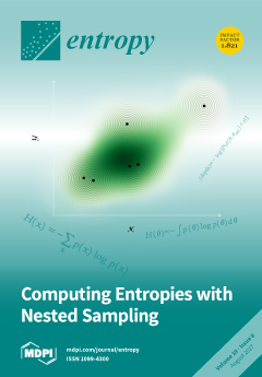
How much uncertainty do we have about a given issue? And how relevant is it to another? Information theory provides a framework for quantifying these notions, in terms of entropy, mutual information, and the like. However, it can be difficult to apply in practice, because difficult integrals appear in the calculations. I adapt the Nested Sampling algorithm used in Bayesian statistics, so that it can calculate information theoretic quantities, making applied information theory easier. View this paper
  • Issues are regarded as officially published after their release is announced to the table of contents alert mailing list.
  • You may sign up for e-mail alerts to receive table of contents of newly released issues.
  • PDF is the official format for papers published in both, html and pdf forms. To view the papers in pdf format, click on the "PDF Full-text" link, and use the free Adobe Reader to open them.
Order results
Result details
Section
Select all
Export citation of selected articles as:
2215 KiB  
Article
Entropy Generation Analysis of Wildfire Propagation
by Elisa Guelpa and Vittorio Verda
Entropy 2017, 19(8), 433; https://doi.org/10.3390/e19080433 - 22 Aug 2017
Cited by 4 | Viewed by 5036
Abstract
Entropy generation is commonly applied to describe the evolution of irreversible processes, such as heat transfer and turbulence. These are both dominating phenomena in fire propagation. In this paper, entropy generation analysis is applied to a grassland fire event, with the aim of [...] Read more.
Entropy generation is commonly applied to describe the evolution of irreversible processes, such as heat transfer and turbulence. These are both dominating phenomena in fire propagation. In this paper, entropy generation analysis is applied to a grassland fire event, with the aim of finding possible links between entropy generation and propagation directions. The ultimate goal of such analysis consists in helping one to overcome possible limitations of the models usually applied to the prediction of wildfire propagation. These models are based on the application of the superimposition of the effects due to wind and slope, which has proven to fail in various cases. The analysis presented here shows that entropy generation allows a detailed analysis of the landscape propagation of a fire and can be thus applied to its quantitative description. Full article
(This article belongs to the Section Thermodynamics)
Show Figures

Graphical abstract

Graphical abstract
Full article ">Figure 1
<p>System illustration.</p>
Full article ">Figure 2
<p>Comparison between landscape propagation models.</p>
Full article ">Figure 3
<p>(<b>a</b>) Control volume example; (<b>b</b>) Main fire front sectors.</p>
Full article ">Figure 4
<p>WFDS simulation results for different slope and wind speed.</p>
Full article ">Figure 5
<p>WFDS simulation results. Temperature evolution at the 26 thermocouple at STATE 1.</p>
Full article ">Figure 6
<p>Entropy flux generated evolution: three contributions.</p>
Full article ">Figure 7
<p>(<b>a</b>) Entropy generated through convection and radiation; (<b>b</b>) Entropy generated through the frontal and the lateral faces.</p>
Full article ">Figure 8
<p>Entropy generated: three contributions.</p>
Full article ">Figure 9
<p>Fire front prediction for STATE 2 through the different analyzed approaches. bold line = fire front; dashed line = entropy generation; grey line = vector composition.</p>
Full article ">
2379 KiB  
Article
Group-Constrained Maximum Correntropy Criterion Algorithms for Estimating Sparse Mix-Noised Channels
by Yanyan Wang, Yingsong Li, Felix Albu and Rui Yang
Entropy 2017, 19(8), 432; https://doi.org/10.3390/e19080432 - 22 Aug 2017
Cited by 36 | Viewed by 4487
Abstract
A group-constrained maximum correntropy criterion (GC-MCC) algorithm is proposed on the basis of the compressive sensing (CS) concept and zero attracting (ZA) techniques and its estimating behavior is verified over sparse multi-path channels. The proposed algorithm is implemented by exerting different norm penalties [...] Read more.
A group-constrained maximum correntropy criterion (GC-MCC) algorithm is proposed on the basis of the compressive sensing (CS) concept and zero attracting (ZA) techniques and its estimating behavior is verified over sparse multi-path channels. The proposed algorithm is implemented by exerting different norm penalties on the two grouped channel coefficients to improve the channel estimation performance in a mixed noise environment. As a result, a zero attraction term is obtained from the expected l 0 and l 1 penalty techniques. Furthermore, a reweighting factor is adopted and incorporated into the zero-attraction term of the GC-MCC algorithm which is denoted as the reweighted GC-MCC (RGC-MMC) algorithm to enhance the estimation performance. Both the GC-MCC and RGC-MCC algorithms are developed to exploit well the inherent sparseness properties of the sparse multi-path channels due to the expected zero-attraction terms in their iterations. The channel estimation behaviors are discussed and analyzed over sparse channels in mixed Gaussian noise environments. The computer simulation results show that the estimated steady-state error is smaller and the convergence is faster than those of the previously reported MCC and sparse MCC algorithms. Full article
Show Figures

Figure 1

Figure 1
<p>Structure diagram of sparse channel estimation.</p>
Full article ">Figure 2
<p>Zero attraction ability of the zero attracting term produced by soft parameter function (SPF), <math display="inline"> <semantics> <msub> <mi>l</mi> <mn>0</mn> </msub> </semantics> </math>-norm and correntropy-induced metric (CIM) penalties.</p>
Full article ">Figure 3
<p>Effects of <math display="inline"> <semantics> <msub> <mi>θ</mi> <mi>GC</mi> </msub> </semantics> </math> on the mean square deviation (MSD) of the proposed GC-MCC algorithm.</p>
Full article ">Figure 4
<p>Effects of <math display="inline"> <semantics> <msub> <mi>θ</mi> <mi>RGC</mi> </msub> </semantics> </math> on the MSD of the proposed RGC-MCC algorithm.</p>
Full article ">Figure 5
<p>MSD performance of the proposed GC-MCC and RGC-MCC algorithms with different <math display="inline"> <semantics> <mi>β</mi> </semantics> </math>.</p>
Full article ">Figure 6
<p>Effects of <math display="inline"> <semantics> <msub> <mi>ε</mi> <mn>1</mn> </msub> </semantics> </math> on the MSD of the proposed GC-MCC and RGC-MCC algorithm.</p>
Full article ">Figure 7
<p>Estimation behavior of the proposed GC-MCC and RGC-MCC algorithms with different SNR.</p>
Full article ">Figure 8
<p>Convergence of the proposed GC-MCC and RGC-MCC algorithms.</p>
Full article ">Figure 9
<p>MSD performance of the proposed GC-MCC and RGC-MCC algorithms for <span class="html-italic">K</span> = 1.</p>
Full article ">Figure 10
<p>MSD performance of the proposed GC-MCC and RGC-MCC algorithms for <span class="html-italic">K</span> = 3.</p>
Full article ">Figure 11
<p>MSD performance of the proposed GC-MCC and RGC-MCC algorithms for <span class="html-italic">K</span> = 5.</p>
Full article ">Figure 12
<p>Estimation behavior of the proposed GC-MCC and RGC-MCC algorithms for estimating a IEEE 802.15.4a channel in CM1 mode.</p>
Full article ">Figure 13
<p>Estimation behavior of the proposed GC-MCC and RGC-MCC algorithms for an echo channel.</p>
Full article ">Figure 14
<p>Features of the soft parameter function with difference <math display="inline"> <semantics> <msub> <mi>τ</mi> <mn>1</mn> </msub> </semantics> </math>.</p>
Full article ">
5968 KiB  
Article
Influence of Failure Probability Due to Parameter and Anchor Variance of a Freeway Dip Slope Slide—A Case Study in Taiwan
by Shong-Loong Chen and Chia-Pang Cheng
Entropy 2017, 19(8), 431; https://doi.org/10.3390/e19080431 - 22 Aug 2017
Cited by 7 | Viewed by 5801
Abstract
The traditional slope stability analysis used the Factor of Safety (FS) from the Limit Equilibrium Theory as the determinant. If the FS was greater than 1, it was considered as “safe” and variables or parameters of uncertainty in the analysis model [...] Read more.
The traditional slope stability analysis used the Factor of Safety (FS) from the Limit Equilibrium Theory as the determinant. If the FS was greater than 1, it was considered as “safe” and variables or parameters of uncertainty in the analysis model were not considered. The objective of research was to analyze the stability of natural slope, in consideration of characteristics of rock layers and the variability of pre-stressing force. By sensitivity and uncertainty analysis, the result showed the sensitivity for pre-stressing force of rock anchor was significantly smaller than the cohesive (c) of rock layer and the varying influence of the friction angle (ϕ) in rock layers. In addition, the immersion by water at the natural slope would weaken the rock layers, in which the cohesion c was reduced to 6 kPa and the friction angle ϕ was decreased below 14°, and it started to show instability and failure in the balance as FS became smaller than 1. The failure rate to the slope could be as high as 50%. By stabilizing with a rock anchor, the failure rate could be reduced below 3%, greatly improving the stability and the reliability of the slope. Full article
Show Figures

Figure 1

Figure 1
<p>Large-scale landslides on a dip slope on the Taiwan Formosan Freeway.</p>
Full article ">Figure 2
<p>The regional geological map at Taiwan Formosan Freeway.</p>
Full article ">Figure 3
<p>Geological profile and geometry of a cross-section of the slope on the Taiwan Formosan Freeway.</p>
Full article ">Figure 4
<p>Geometry of a slope for plane failure.</p>
Full article ">Figure 5
<p>Schematic of the three Point Estimate Methods (PEMs) in a standardized parameter space for a bivariate case.</p>
Full article ">Figure 6
<p>Univariate sensitivity analysis when <span class="html-italic">c</span> = 59 kPa and <span class="html-italic">ϕ</span> = 30°.</p>
Full article ">Figure 7
<p>Univariate sensitivity analysis when <span class="html-italic">c</span> = 10 kPa and <span class="html-italic">ϕ</span> = 30°.</p>
Full article ">Figure 8
<p>Sensitivity <span class="html-italic">ϕ</span> = <span class="html-italic">c</span> test.</p>
Full article ">Figure 8 Cont.
<p>Sensitivity <span class="html-italic">ϕ</span> = <span class="html-italic">c</span> test.</p>
Full article ">Figure 8 Cont.
<p>Sensitivity <span class="html-italic">ϕ</span> = <span class="html-italic">c</span> test.</p>
Full article ">Figure 9
<p><span class="html-italic">C<sub>ϕC</sub></span> linear function.</p>
Full article ">Figure 10
<p>Factor of safety contour map.</p>
Full article ">Figure 11
<p>Failure probability before and after immersion (without anchor).</p>
Full article ">Figure 12
<p>Failure probability before and after immersion (with anchor).</p>
Full article ">Figure 13
<p>Relationship between correlation coefficient (<span class="html-italic">ρ</span>) and failure probability (<span class="html-italic">Pf</span>).</p>
Full article ">
304 KiB  
Article
Logical Entropy and Logical Mutual Information of Experiments in the Intuitionistic Fuzzy Case
by Dagmar Markechová and Beloslav Riečan
Entropy 2017, 19(8), 429; https://doi.org/10.3390/e19080429 - 21 Aug 2017
Cited by 12 | Viewed by 4604
Abstract
In this contribution, we introduce the concepts of logical entropy and logical mutual information of experiments in the intuitionistic fuzzy case, and study the basic properties of the suggested measures. Subsequently, by means of the suggested notion of logical entropy of an IF-partition, [...] Read more.
In this contribution, we introduce the concepts of logical entropy and logical mutual information of experiments in the intuitionistic fuzzy case, and study the basic properties of the suggested measures. Subsequently, by means of the suggested notion of logical entropy of an IF-partition, we define the logical entropy of an IF-dynamical system. It is shown that the logical entropy of IF-dynamical systems is invariant under isomorphism. Finally, an analogy of the Kolmogorov–Sinai theorem on generators for IF-dynamical systems is proved. Full article
(This article belongs to the Special Issue Entropy and Its Applications across Disciplines)
227 KiB  
Article
The Potential Application of Multiscale Entropy Analysis of Electroencephalography in Children with Neurological and Neuropsychiatric Disorders
by Yen-Ju Chu, Chi-Feng Chang, Jiann-Shing Shieh and Wang-Tso Lee
Entropy 2017, 19(8), 428; https://doi.org/10.3390/e19080428 - 21 Aug 2017
Cited by 17 | Viewed by 5368
Abstract
Electroencephalography (EEG) is frequently used in functional neurological assessment of children with neurological and neuropsychiatric disorders. Multiscale entropy (MSE) can reveal complexity in both short and long time scales and is more feasible in the analysis of EEG. Entropy-based estimation of EEG complexity [...] Read more.
Electroencephalography (EEG) is frequently used in functional neurological assessment of children with neurological and neuropsychiatric disorders. Multiscale entropy (MSE) can reveal complexity in both short and long time scales and is more feasible in the analysis of EEG. Entropy-based estimation of EEG complexity is a powerful tool in investigating the underlying disturbances of neural networks of the brain. Most neurological and neuropsychiatric disorders in childhood affect the early stage of brain development. The analysis of EEG complexity may show the influences of different neurological and neuropsychiatric disorders on different regions of the brain during development. This article aims to give a brief summary of current concepts of MSE analysis in pediatric neurological and neuropsychiatric disorders. Studies utilizing MSE or its modifications for investigating neurological and neuropsychiatric disorders in children were reviewed. Abnormal EEG complexity was shown in a variety of childhood neurological and neuropsychiatric diseases, including autism, attention deficit/hyperactivity disorder, Tourette syndrome, and epilepsy in infancy and childhood. MSE has been shown to be a powerful method for analyzing the non-linear anomaly of EEG in childhood neurological diseases. Further studies are needed to show its clinical implications on diagnosis, treatment, and outcome prediction. Full article
(This article belongs to the Special Issue Entropy and Electroencephalography II)
3212 KiB  
Article
Minimum and Maximum Entropy Distributions for Binary Systems with Known Means and Pairwise Correlations
by Badr F. Albanna, Christopher Hillar, Jascha Sohl-Dickstein and Michael R. DeWeese
Entropy 2017, 19(8), 427; https://doi.org/10.3390/e19080427 - 21 Aug 2017
Cited by 4 | Viewed by 8050
Abstract
Maximum entropy models are increasingly being used to describe the collective activity of neural populations with measured mean neural activities and pairwise correlations, but the full space of probability distributions consistent with these constraints has not been explored. We provide upper and lower [...] Read more.
Maximum entropy models are increasingly being used to describe the collective activity of neural populations with measured mean neural activities and pairwise correlations, but the full space of probability distributions consistent with these constraints has not been explored. We provide upper and lower bounds on the entropy for the minimum entropy distribution over arbitrarily large collections of binary units with any fixed set of mean values and pairwise correlations. We also construct specific low-entropy distributions for several relevant cases. Surprisingly, the minimum entropy solution has entropy scaling logarithmically with system size for any set of first- and second-order statistics consistent with arbitrarily large systems. We further demonstrate that some sets of these low-order statistics can only be realized by small systems. Our results show how only small amounts of randomness are needed to mimic low-order statistical properties of highly entropic distributions, and we discuss some applications for engineered and biological information transmission systems. Full article
(This article belongs to the Special Issue Thermodynamics of Information Processing)
Show Figures

Figure 1

Figure 1
<p>Minimum and maximum entropy for fixed uniform constraints as a function of <span class="html-italic">N</span>. The minimum entropy grows no faster than logarithmically with the system size <span class="html-italic">N</span> for any mean activity level <math display="inline"> <semantics> <mi>μ</mi> </semantics> </math> and pairwise correlation strength <math display="inline"> <semantics> <mi>ν</mi> </semantics> </math>. (<b>a</b>) In a parameter regime relevant for neural population activity in the retina [<a href="#B5-entropy-19-00427" class="html-bibr">5</a>,<a href="#B6-entropy-19-00427" class="html-bibr">6</a>] (<math display="inline"> <semantics> <mrow> <mi>μ</mi> <mo>=</mo> <mn>0.1</mn> </mrow> </semantics> </math>, <math display="inline"> <semantics> <mrow> <mi>ν</mi> <mo>=</mo> <mn>0.011</mn> </mrow> </semantics> </math>), we can construct an explicit low entropy solution (<math display="inline"> <semantics> <msubsup> <mover accent="true"> <mi>S</mi> <mo stretchy="false">˜</mo> </mover> <mn>2</mn> <mrow> <mi>c</mi> <mi>o</mi> <mi>n</mi> <mn>2</mn> </mrow> </msubsup> </semantics> </math>) that grows logarithmically with <span class="html-italic">N</span>, unlike the linear behavior of the maximum entropy solution (<math display="inline"> <semantics> <msub> <mi>S</mi> <mn>2</mn> </msub> </semantics> </math>). Note that the linear behavior of the maximum entropy solution is only possible because these parameter values remain within the boundary of allowed <math display="inline"> <semantics> <mi>μ</mi> </semantics> </math> and <math display="inline"> <semantics> <mi>ν</mi> </semantics> </math> values (See <a href="#app3-entropy-19-00427" class="html-app">Appendix C</a>); (<b>b</b>) Even for mean activities and pairwise correlations matched to the global maximum entropy solution (<math display="inline"> <semantics> <msub> <mi>S</mi> <mn>2</mn> </msub> </semantics> </math>; <math display="inline"> <semantics> <mrow> <mi>μ</mi> <mo>=</mo> <mfrac bevelled="true"> <mn>1</mn> <mn>2</mn> </mfrac> </mrow> </semantics> </math>, <math display="inline"> <semantics> <mrow> <mi>ν</mi> <mo>=</mo> <mfrac bevelled="true"> <mn>1</mn> <mn>4</mn> </mfrac> </mrow> </semantics> </math>), we can construct explicit low entropy solutions (<math display="inline"> <semantics> <msubsup> <mover accent="true"> <mi>S</mi> <mo stretchy="false">˜</mo> </mover> <mn>2</mn> <mrow> <mi>c</mi> <mi>o</mi> <mi>n</mi> </mrow> </msubsup> </semantics> </math> and <math display="inline"> <semantics> <msubsup> <mover accent="true"> <mi>S</mi> <mo stretchy="false">˜</mo> </mover> <mn>2</mn> <mrow> <mi>c</mi> <mi>o</mi> <mi>n</mi> <mn>2</mn> </mrow> </msubsup> </semantics> </math>) and a lower bound (<math display="inline"> <semantics> <msubsup> <mover accent="true"> <mi>S</mi> <mo stretchy="false">˜</mo> </mover> <mn>2</mn> <mrow> <mi>l</mi> <mi>o</mi> </mrow> </msubsup> </semantics> </math>) on the entropy that each grow logarithmically with <span class="html-italic">N</span>, in contrast to the linear behavior of the maximum entropy solution (<math display="inline"> <semantics> <msub> <mi>S</mi> <mn>2</mn> </msub> </semantics> </math>) and the finitely exchangeable minimum entropy solution (<math display="inline"> <semantics> <msubsup> <mover accent="true"> <mi>S</mi> <mo stretchy="false">˜</mo> </mover> <mn>2</mn> <mrow> <mi>e</mi> <mi>x</mi> <mi>c</mi> <mi>h</mi> </mrow> </msubsup> </semantics> </math>). <math display="inline"> <semantics> <msub> <mover accent="true"> <mi>S</mi> <mo stretchy="false">˜</mo> </mover> <mn>1</mn> </msub> </semantics> </math> is the minimum entropy distribution that is consistent with the mean firing rates. It remains constant as a function of <span class="html-italic">N</span>.</p>
Full article ">Figure 2
<p>Minimum and maximum entropy models for uniform constraints. (<b>a</b>) Entropy as a function of the strength of pairwise correlations for the maximum entropy model (<math display="inline"> <semantics> <msub> <mi>S</mi> <mn>2</mn> </msub> </semantics> </math>), finitely exchangeable minimum entropy model (<math display="inline"> <semantics> <msubsup> <mover accent="true"> <mi>S</mi> <mo stretchy="false">˜</mo> </mover> <mn>2</mn> <mrow> <mi>e</mi> <mi>x</mi> <mi>c</mi> <mi>h</mi> </mrow> </msubsup> </semantics> </math>), and a constructed low entropy solution (<math display="inline"> <semantics> <msubsup> <mover accent="true"> <mi>S</mi> <mo stretchy="false">˜</mo> </mover> <mn>2</mn> <mrow> <mi>c</mi> <mi>o</mi> <mi>n</mi> </mrow> </msubsup> </semantics> </math>), all corresponding to <math display="inline"> <semantics> <mrow> <mi>μ</mi> <mo>=</mo> <mfrac bevelled="true"> <mn>1</mn> <mn>2</mn> </mfrac> </mrow> </semantics> </math> and <math display="inline"> <semantics> <mrow> <mi>N</mi> <mo>=</mo> <mn>5</mn> </mrow> </semantics> </math>. Filled circles indicate the global minimum <math display="inline"> <semantics> <msub> <mover accent="true"> <mi>S</mi> <mo stretchy="false">˜</mo> </mover> <mn>1</mn> </msub> </semantics> </math> and maximum <math display="inline"> <semantics> <msub> <mi>S</mi> <mn>1</mn> </msub> </semantics> </math> for <math display="inline"> <semantics> <mrow> <mi>μ</mi> <mo>=</mo> <mfrac bevelled="true"> <mn>1</mn> <mn>2</mn> </mfrac> </mrow> </semantics> </math>; (<b>b</b>–<b>d</b>) Support for <math display="inline"> <semantics> <msub> <mi>S</mi> <mn>2</mn> </msub> </semantics> </math> (b), <math display="inline"> <semantics> <msubsup> <mover accent="true"> <mi>S</mi> <mo stretchy="false">˜</mo> </mover> <mn>2</mn> <mrow> <mi>e</mi> <mi>x</mi> <mi>c</mi> <mi>h</mi> </mrow> </msubsup> </semantics> </math> (c), and <math display="inline"> <semantics> <msubsup> <mover accent="true"> <mi>S</mi> <mo stretchy="false">˜</mo> </mover> <mn>2</mn> <mrow> <mi>c</mi> <mi>o</mi> <mi>n</mi> </mrow> </msubsup> </semantics> </math> (d) corresponding to the three curves in panel (a). States are grouped by the number of active units; darker regions indicate higher total probability for each group of states; (<b>e</b>–<b>h</b>) Same as for panels (a) through (d), but with <math display="inline"> <semantics> <mrow> <mi>N</mi> <mo>=</mo> <mn>30</mn> </mrow> </semantics> </math>. Note that, with rising <span class="html-italic">N</span>, the cusps in the <math display="inline"> <semantics> <msubsup> <mover accent="true"> <mi>S</mi> <mo stretchy="false">˜</mo> </mover> <mn>2</mn> <mrow> <mi>e</mi> <mi>x</mi> <mi>c</mi> <mi>h</mi> </mrow> </msubsup> </semantics> </math> curve become much less pronounced.</p>
Full article ">Figure 3
<p>An example of uniform, low-level statistics that can be realized by small groups of neurons but not by any system greater than some critical size. (<b>a</b>) Upper (red curve, <math display="inline"> <semantics> <msub> <mover accent="true"> <mi>ν</mi> <mo stretchy="false">˜</mo> </mover> <mrow> <mi>u</mi> <mi>p</mi> <mi>p</mi> <mi>e</mi> <mi>r</mi> </mrow> </msub> </semantics> </math>) and lower (cyan curve, <math display="inline"> <semantics> <msub> <mover accent="true"> <mi>ν</mi> <mo stretchy="false">˜</mo> </mover> <mrow> <mi>l</mi> <mi>o</mi> <mi>w</mi> <mi>e</mi> <mi>r</mi> </mrow> </msub> </semantics> </math>) bounds on the minimum value (black curve, <math display="inline"> <semantics> <mover accent="true"> <mi>ν</mi> <mo stretchy="false">˜</mo> </mover> </semantics> </math>) for the pairwise correlation <math display="inline"> <semantics> <mi>ν</mi> </semantics> </math> shared by all pairs of neurons are plotted as a function of system size <span class="html-italic">N</span> assuming that every neuron has mean activity <math display="inline"> <semantics> <mrow> <mi>μ</mi> <mo>=</mo> <mn>0.1</mn> </mrow> </semantics> </math>. Note that all three curves asymptote to <math display="inline"> <semantics> <mrow> <mi>ν</mi> <mo>=</mo> <msup> <mi>μ</mi> <mn>2</mn> </msup> <mo>=</mo> <mn>0.01</mn> </mrow> </semantics> </math> as <math display="inline"> <semantics> <mrow> <mi>N</mi> <mo>→</mo> <mo>∞</mo> </mrow> </semantics> </math> (dashed blue line); (<b>b</b>) Enlarged portion of (<b>a</b>) outlined in grey reveals that groups of <math display="inline"> <semantics> <mrow> <mi>N</mi> <mo>≤</mo> <mn>150</mn> </mrow> </semantics> </math> neurons can exhibit uniform constraints <math display="inline"> <semantics> <mrow> <mi>μ</mi> <mo>=</mo> <mn>0.1</mn> </mrow> </semantics> </math> and <math display="inline"> <semantics> <mrow> <mi>ν</mi> <mo>=</mo> <mn>0.0094</mn> </mrow> </semantics> </math> (green dotted line), but this is not possible for any larger group.</p>
Full article ">Figure 4
<p>An example of the allowed values of <math display="inline"> <semantics> <msub> <mi>λ</mi> <mn>0</mn> </msub> </semantics> </math> and <math display="inline"> <semantics> <msub> <mi>λ</mi> <mn>1</mn> </msub> </semantics> </math> for the dual problem (<math display="inline"> <semantics> <mrow> <mi>N</mi> <mo>=</mo> <mn>5</mn> </mrow> </semantics> </math>).</p>
Full article ">Figure 5
<p>The red shaded region is the set of values for <math display="inline"> <semantics> <mi>μ</mi> </semantics> </math> and <math display="inline"> <semantics> <mi>ν</mi> </semantics> </math> that can be satisfied for at least one probability distribution in the <math display="inline"> <semantics> <mrow> <mi>N</mi> <mo>→</mo> <mo>∞</mo> </mrow> </semantics> </math> limit. The purple line along the diagonal where <math display="inline"> <semantics> <mrow> <mi>ν</mi> <mo>=</mo> <mi>μ</mi> </mrow> </semantics> </math> is the distribution for which only the all active and all inactive states have non-zero probability. It represents the global entropy minimum for a given value of <math display="inline"> <semantics> <mi>μ</mi> </semantics> </math>. The red parabola, <math display="inline"> <semantics> <mrow> <mi>ν</mi> <mo>=</mo> <msup> <mi>μ</mi> <mn>2</mn> </msup> </mrow> </semantics> </math>, at the bottom border of the allowed region corresponds to a wide range of probability distributions, including the global maximum entropy solution for given <math display="inline"> <semantics> <mi>μ</mi> </semantics> </math> in which each neuron fires independently. We find that low entropy solutions reside at this low <math display="inline"> <semantics> <mi>ν</mi> </semantics> </math> boundary as well.</p>
Full article ">Figure 6
<p>For the case of uniform constraints achievable by arbitrarily large systems, the maximum possible entropy scales linearly with system size, <span class="html-italic">N</span>, as shown here for various values of <math display="inline"> <semantics> <mi>μ</mi> </semantics> </math> and <math display="inline"> <semantics> <mi>ν</mi> </semantics> </math>. Note that this linear scaling holds even for large correlations, provided that <math display="inline"> <semantics> <mrow> <mi>ν</mi> <mo>&lt;</mo> <mi>μ</mi> </mrow> </semantics> </math>. For the extreme case <math display="inline"> <semantics> <mrow> <mi>ν</mi> <mo>=</mo> <mi>μ</mi> </mrow> </semantics> </math>, all the neurons are perfectly correlated so the entropy of the ensemble does not change with increasing <span class="html-italic">N</span>.</p>
Full article ">Figure 7
<p>The minimum entropy for exchangeable distributions versus <span class="html-italic">N</span> for various values of <math display="inline"> <semantics> <mi>μ</mi> </semantics> </math> and <math display="inline"> <semantics> <mi>ν</mi> </semantics> </math>. Note that, like the maximum entropy, the exchangeable minimum entropy scales linearly with <span class="html-italic">N</span> as <math display="inline"> <semantics> <mrow> <mi>N</mi> <mo>→</mo> <mo>∞</mo> </mrow> </semantics> </math>, albeit with a smaller slope for <math display="inline"> <semantics> <mrow> <mi>ν</mi> <mo>≠</mo> <msup> <mi>μ</mi> <mn>2</mn> </msup> </mrow> </semantics> </math>. We can calculate the entropy exactly for <math display="inline"> <semantics> <mi>μ</mi> </semantics> </math> = 0.5 and <math display="inline"> <semantics> <mi>ν</mi> </semantics> </math> = 0.25 as <math display="inline"> <semantics> <mrow> <mi>N</mi> <mo>→</mo> <mo>∞</mo> </mrow> </semantics> </math>, and we find that the leading term is indeed linear: <math display="inline"> <semantics> <mrow> <msubsup> <mover accent="true"> <mi>S</mi> <mo stretchy="false">˜</mo> </mover> <mn>2</mn> <mrow> <mi>e</mi> <mi>x</mi> <mi>c</mi> <mi>h</mi> </mrow> </msubsup> <mo>≈</mo> <mi>N</mi> <mo>−</mo> <mn>1</mn> <mo>/</mo> <mn>2</mn> <msub> <mo form="prefix">log</mo> <mn>2</mn> </msub> <mrow> <mo>(</mo> <mi>N</mi> <mo>)</mo> </mrow> <mo>−</mo> <mn>1</mn> <mo>/</mo> <mn>2</mn> <msub> <mo form="prefix">log</mo> <mn>2</mn> </msub> <mrow> <mo>(</mo> <mn>2</mn> <mi>π</mi> <mo>)</mo> </mrow> <mo>+</mo> <mi>O</mi> <mrow> <mo>[</mo> <msub> <mo form="prefix">log</mo> <mn>2</mn> </msub> <mrow> <mo>(</mo> <mi>N</mi> <mo>)</mo> </mrow> <mo>/</mo> <mi>N</mi> <mo>]</mo> </mrow> </mrow> </semantics> </math>.</p>
Full article ">Figure 8
<p>The full shaded region includes all allowed values for the constraints <math display="inline"> <semantics> <mi>μ</mi> </semantics> </math> and <math display="inline"> <semantics> <mi>ν</mi> </semantics> </math> for all possible probability distributions, replotted from <a href="#entropy-19-00427-f005" class="html-fig">Figure A2</a>. As described in <a href="#app5-entropy-19-00427" class="html-app">Appendix E</a> and <a href="#app7-entropy-19-00427" class="html-app">Appendix G</a>, one of our low-entropy constructed solutions can be matched to any of the allowed constraint values in the full shaded region, whereas the constructed solution described in <a href="#app6-entropy-19-00427" class="html-app">Appendix F</a> can achieve any of the values within the triangular purple shaded region. Note that even with this second solution, we can cover most of the allowed region. Each of our constructed solutions have entropies that scale as <math display="inline"> <semantics> <mrow> <mi>S</mi> <mo>∼</mo> <mo form="prefix">ln</mo> <mo>(</mo> <mi>N</mi> <mo>)</mo> </mrow> </semantics> </math>.</p>
Full article ">
1038 KiB  
Article
Iterative QR-Based SFSIC Detection and Decoder Algorithm for a Reed–Muller Space-Time Turbo System
by Liang-Fang Ni, Yi Wang, Wei-Xia Li, Pei-Zhen Wang and Jia-Yan Zhang
Entropy 2017, 19(8), 426; https://doi.org/10.3390/e19080426 - 20 Aug 2017
Cited by 1 | Viewed by 4257
Abstract
An iterative QR-based soft feedback segment interference cancellation (QRSFSIC) detection and decoder algorithm for a Reed–Muller (RM) space-time turbo system is proposed in this paper. It forms the sufficient statistic for the minimum-mean-square error (MMSE) estimate according to QR decomposition-based soft feedback successive [...] Read more.
An iterative QR-based soft feedback segment interference cancellation (QRSFSIC) detection and decoder algorithm for a Reed–Muller (RM) space-time turbo system is proposed in this paper. It forms the sufficient statistic for the minimum-mean-square error (MMSE) estimate according to QR decomposition-based soft feedback successive interference cancellation, stemmed from the a priori log-likelihood ratio (LLR) of encoded bits. Then, the signal originating from the symbols of the reliable segment, the symbol reliability metric, in terms of an a posteriori LLR of encoded bits which is larger than a certain threshold, is iteratively cancelled with the QRSFSIC in order to further obtain the residual signal for evaluating the symbols in the unreliable segment. This is done until the unreliable segment is empty, resulting in the extrinsic information for a RM turbo-coded bit with the greatest likelihood. Bridged by de-multiplexing and multiplexing, an iterative QRSFSIC detection is concatenated with an iterative trellis-based maximum a posteriori probability RM turbo decoder as if a principal Turbo detection and decoder is embedded with an iterative subordinate QRSFSIC detection and a RM turbo decoder, exchanging each other’s detection and decoding soft-decision information iteratively. These three stages let the proposed algorithm approach the upper bound of the diversity. The simulation results also show that the proposed scheme outperforms the other suboptimum detectors considered in this paper. Full article
(This article belongs to the Section Information Theory, Probability and Statistics)
Show Figures

Figure 1

Figure 1
<p>The configuration of a Reed–Muller space-time turbo system with a receiver based on a QR-based SFSIC detector and decoder.</p>
Full article ">Figure 2
<p>Internal structure of the RM-turbo decoder.</p>
Full article ">Figure 3
<p>The BERs of the IQRSFSICDD versus SNR values over a range of iterations, with the transmitters using the 4-QAM and (<b>a</b>) the R = 121/240 outer channel RM turbo code for <span class="html-italic">N<sub>t</sub></span> = <span class="html-italic">N<sub>r</sub></span> = 3 (<b>left</b>); and (<b>b</b>) the R = 676/988 outer channel RM turbo code for <span class="html-italic">N<sub>t</sub></span> = <span class="html-italic">N<sub>r</sub></span> = 4 (<b>right</b>).</p>
Full article ">Figure 4
<p>The BERs of three iterative detection schemes versus SNR values, with the transmitters using the 4-QAM and: (<b>a</b>) R = 121/240 outer channel RM turbo code for <span class="html-italic">N<sub>t</sub></span> = <span class="html-italic">N<sub>r</sub></span> = 3 (<b>left</b>); (<b>b</b>) R = 676/988 outer channel RM turbo code for <span class="html-italic">N<sub>t</sub></span> = <span class="html-italic">N<sub>r</sub></span> = 4 (<b>right</b>).</p>
Full article ">
6929 KiB  
Article
A Sparse Multiwavelet-Based Generalized Laguerre–Volterra Model for Identifying Time-Varying Neural Dynamics from Spiking Activities
by Song Xu, Yang Li, Tingwen Huang and Rosa H. M. Chan
Entropy 2017, 19(8), 425; https://doi.org/10.3390/e19080425 - 20 Aug 2017
Cited by 7 | Viewed by 5611
Abstract
Modeling of a time-varying dynamical system provides insights into the functions of biological neural networks and contributes to the development of next-generation neural prostheses. In this paper, we have formulated a novel sparse multiwavelet-based generalized Laguerre–Volterra (sMGLV) modeling framework to identify the time-varying [...] Read more.
Modeling of a time-varying dynamical system provides insights into the functions of biological neural networks and contributes to the development of next-generation neural prostheses. In this paper, we have formulated a novel sparse multiwavelet-based generalized Laguerre–Volterra (sMGLV) modeling framework to identify the time-varying neural dynamics from multiple spike train data. First, the significant inputs are selected by using a group least absolute shrinkage and selection operator (LASSO) method, which can capture the sparsity within the neural system. Second, the multiwavelet-based basis function expansion scheme with an efficient forward orthogonal regression (FOR) algorithm aided by mutual information is utilized to rapidly capture the time-varying characteristics from the sparse model. Quantitative simulation results demonstrate that the proposed sMGLV model in this paper outperforms the initial full model and the state-of-the-art modeling methods in tracking performance for various time-varying kernels. Analyses of experimental data show that the proposed sMGLV model can capture the timing of transient changes accurately. The proposed framework will be useful to the study of how, when, and where information transmission processes across brain regions evolve in behavior. Full article
(This article belongs to the Special Issue Entropy in Signal Analysis)
Show Figures

Figure 1

Figure 1
<p>Schematic diagram of the sMGLV framework.</p>
Full article ">Figure 2
<p>The structures of the time-varying MIMO and MISO neural spiking system. (<b>a</b>) the MIMO neural spiking system with the sparse connectivity among the neural population. The solid lines represent the causal relationship between the input and output spiking signals. The dashed lines indicate that there is no causal relationship between them; (<b>b</b>) the structurally plausible time-varying MISO neural spiking model.</p>
Full article ">Figure 3
<p>Laguerre basis functions (first to 15th order). The Laguerre parameters <span class="html-italic">L</span> equals 15 and <math display="inline"> <semantics> <mi>β</mi> </semantics> </math> equals 0.7.</p>
Full article ">Figure 4
<p>Multiwavelet B-splines with the same scale <math display="inline"> <semantics> <mrow> <mi>j</mi> <mo>=</mo> <mn>3</mn> </mrow> </semantics> </math>, and different orders as 2, 3, 4, 5.</p>
Full article ">Figure 5
<p>The estimations of time-varying kernels from an 8-input 1-output system using the dMGLV and the proposed sMGLV modeling methods, where the true kernels are given at 400 s and 800 s, respectively, in two stages. (<b>a</b>) comparing estimation results for different kernels using the dMGLV model and sMGLV model in the first half of the time course; (<b>b</b>) comparing estimation results for different kernels using the dMGLV model and sMGLV model in the second half of the time course</p>
Full article ">Figure 5 Cont.
<p>The estimations of time-varying kernels from an 8-input 1-output system using the dMGLV and the proposed sMGLV modeling methods, where the true kernels are given at 400 s and 800 s, respectively, in two stages. (<b>a</b>) comparing estimation results for different kernels using the dMGLV model and sMGLV model in the first half of the time course; (<b>b</b>) comparing estimation results for different kernels using the dMGLV model and sMGLV model in the second half of the time course</p>
Full article ">Figure 6
<p>Kernel shapes for a first-order, 8-input, single-output system with step and linear changes using four different algorithms across simulation time evolution in 2D. The feedback kernel considered in the system can be written as <math display="inline"> <semantics> <msup> <mi>k</mi> <mrow> <mo>(</mo> <mn>9</mn> <mo>)</mo> </mrow> </msup> </semantics> </math>. The amplitudes of the kernels are color-coded.</p>
Full article ">Figure 7
<p>Peak amplitudes of actual kernels (black) and estimated kernels (blue for SSPPF, green for sSSPPF, purple for dMGLV, and red for the proposed sMGLV model) across simulation time evolution in a time-varying system with a 1 s resolution.</p>
Full article ">Figure 8
<p>Estimated output spike train and correlation plot. (<b>a</b>) Estimated output spike train calculated using the proposed sMGLV model. The first row is the estimated firing probability intensity; the second row is the estimated output spike train; the third row is the corresponding actual spike train fragment. (<b>b</b>) Correlation plot. The correlation coefficient <span class="html-italic">r</span> for the whole simulation data length is calculated as a function of the standard deviation <math display="inline"> <semantics> <msub> <mi>σ</mi> <mi>g</mi> </msub> </semantics> </math> of the Gaussian smoothing kernel.</p>
Full article ">Figure 9
<p>The estimations of a 4-input and 1-output retina model using the proposed sMGLV modelling method. Estimated kernels using the sMGLV model at different times are drawn with different colors in the left figure; amplitudes and the corresponding stand errors for the estimated kernels can be seen in the right figure.</p>
Full article ">
589 KiB  
Article
Survey on Probabilistic Models of Low-Rank Matrix Factorizations
by Jiarong Shi, Xiuyun Zheng and Wei Yang
Entropy 2017, 19(8), 424; https://doi.org/10.3390/e19080424 - 19 Aug 2017
Cited by 13 | Viewed by 6266
Abstract
Low-rank matrix factorizations such as Principal Component Analysis (PCA), Singular Value Decomposition (SVD) and Non-negative Matrix Factorization (NMF) are a large class of methods for pursuing the low-rank approximation of a given data matrix. The conventional factorization models are based on the assumption [...] Read more.
Low-rank matrix factorizations such as Principal Component Analysis (PCA), Singular Value Decomposition (SVD) and Non-negative Matrix Factorization (NMF) are a large class of methods for pursuing the low-rank approximation of a given data matrix. The conventional factorization models are based on the assumption that the data matrices are contaminated stochastically by some type of noise. Thus the point estimations of low-rank components can be obtained by Maximum Likelihood (ML) estimation or Maximum a posteriori (MAP). In the past decade, a variety of probabilistic models of low-rank matrix factorizations have emerged. The most significant difference between low-rank matrix factorizations and their corresponding probabilistic models is that the latter treat the low-rank components as random variables. This paper makes a survey of the probabilistic models of low-rank matrix factorizations. Firstly, we review some probability distributions commonly-used in probabilistic models of low-rank matrix factorizations and introduce the conjugate priors of some probability distributions to simplify the Bayesian inference. Then we provide two main inference methods for probabilistic low-rank matrix factorizations, i.e., Gibbs sampling and variational Bayesian inference. Next, we classify roughly the important probabilistic models of low-rank matrix factorizations into several categories and review them respectively. The categories are performed via different matrix factorizations formulations, which mainly include PCA, matrix factorizations, robust PCA, NMF and tensor factorizations. Finally, we discuss the research issues needed to be studied in the future. Full article
(This article belongs to the Special Issue Information Theory in Machine Learning and Data Science)
Show Figures

Figure 1

Figure 1
<p>Relationships among several probability distributions.</p>
Full article ">
1463 KiB  
Article
An Improved System for Utilizing Low-Temperature Waste Heat of Flue Gas from Coal-Fired Power Plants
by Shengwei Huang, Chengzhou Li, Tianyu Tan, Peng Fu, Gang Xu and Yongping Yang
Entropy 2017, 19(8), 423; https://doi.org/10.3390/e19080423 - 19 Aug 2017
Cited by 23 | Viewed by 7551
Abstract
In this paper, an improved system to efficiently utilize the low-temperature waste heat from the flue gas of coal-fired power plants is proposed based on heat cascade theory. The essence of the proposed system is that the waste heat of exhausted flue gas [...] Read more.
In this paper, an improved system to efficiently utilize the low-temperature waste heat from the flue gas of coal-fired power plants is proposed based on heat cascade theory. The essence of the proposed system is that the waste heat of exhausted flue gas is not only used to preheat air for assisting coal combustion as usual but also to heat up feedwater and for low-pressure steam extraction. Air preheating is performed by both the exhaust flue gas in the boiler island and the low-pressure steam extraction in the turbine island; thereby part of the flue gas heat originally exchanged in the air preheater can be saved and introduced to heat the feedwater and the high-temperature condensed water. Consequently, part of the high-pressure steam is saved for further expansion in the steam turbine, which results in additional net power output. Based on the design data of a typical 1000 MW ultra-supercritical coal-fired power plant in China, an in-depth analysis of the energy-saving characteristics of the improved waste heat utilization system (WHUS) and the conventional WHUS is conducted. When the improved WHUS is adopted in a typical 1000 MW unit, net power output increases by 19.51 MW, exergy efficiency improves to 45.46%, and net annual revenue reaches USD 4.741 million while for the conventional WHUS, these performance parameters are 5.83 MW, 44.80% and USD 1.244 million, respectively. The research described in this paper provides a feasible energy-saving option for coal-fired power plants. Full article
(This article belongs to the Special Issue Work Availability and Exergy Analysis)
Show Figures

Figure 1

Figure 1
<p>Schematic of the waste heat utilization system (WHUS).</p>
Full article ">Figure 2
<p>Schematic of the considered coal-fired power plant with a conventional heat recovery system.</p>
Full article ">Figure 3
<p>Heat transfer curve of the conventional WHUS.</p>
Full article ">Figure 4
<p>Schematic of the thermal system of a power plant with the improved WHUS.</p>
Full article ">Figure 5
<p>Heat transfer curve of the improved WHUS.</p>
Full article ">Figure 6
<p>Effects of waste heat utilization on the steam turbine regenerative heaters. (<b>a</b>) The conventional WHUS; (<b>b</b>) The improved WHUS.</p>
Full article ">Figure 6 Cont.
<p>Effects of waste heat utilization on the steam turbine regenerative heaters. (<b>a</b>) The conventional WHUS; (<b>b</b>) The improved WHUS.</p>
Full article ">
782 KiB  
Article
Computing Entropies with Nested Sampling
by Brendon J. Brewer
Entropy 2017, 19(8), 422; https://doi.org/10.3390/e19080422 - 18 Aug 2017
Cited by 8 | Viewed by 6221
Abstract
The Shannon entropy, and related quantities such as mutual information, can be used to quantify uncertainty and relevance. However, in practice, it can be difficult to compute these quantities for arbitrary probability distributions, particularly if the probability mass functions or densities cannot be [...] Read more.
The Shannon entropy, and related quantities such as mutual information, can be used to quantify uncertainty and relevance. However, in practice, it can be difficult to compute these quantities for arbitrary probability distributions, particularly if the probability mass functions or densities cannot be evaluated. This paper introduces a computational approach, based on Nested Sampling, to evaluate entropies of probability distributions that can only be sampled. I demonstrate the method on three examples: a simple Gaussian example where the key quantities are available analytically; (ii) an experimental design example about scheduling observations in order to measure the period of an oscillating signal; and (iii) predicting the future from the past in a heavy-tailed scenario. Full article
(This article belongs to the Special Issue Maximum Entropy and Bayesian Methods)
Show Figures

Figure 1

Figure 1
<p>To evaluate the log-probability (or density) of the blue probability distribution near the red point, Nested Sampling can be used, with the blue distribution playing the role of the “prior” in NS, and the Euclidean distance from the red point (illustrated with red contours) playing the role of the negative log-likelihood. Averaging over selections of the red point gives an estimate of the entropy of the blue distribution.</p>
Full article ">Figure 2
<p>A signal with true parameters <math display="inline"> <semantics> <mrow> <mi>A</mi> <mo>=</mo> <mn>1</mn> </mrow> </semantics> </math>, <math display="inline"> <semantics> <mrow> <mi>τ</mi> <mo>=</mo> <mo>−</mo> <mn>0.5</mn> </mrow> </semantics> </math>, and <math display="inline"> <semantics> <mrow> <mi>ϕ</mi> <mo>=</mo> <mn>0</mn> </mrow> </semantics> </math>, observed with noise standard deviation 0.1 with the even (gold points) and uneven (green points) observing strategies.</p>
Full article ">Figure 3
<p>The joint distribution for the log-sum of the first half of the ‘Pareto data’ and the second half. The goal is to calculate the entropy of the marginal distributions, the entropy of the joint distribution, and hence the mutual information. The distribution is quite heavy tailed despite the logarithms, and extends beyond the domain shown in this plot.</p>
Full article ">
3013 KiB  
Article
Incipient Fault Diagnosis of Rolling Bearings Based on Impulse-Step Impact Dictionary and Re-Weighted Minimizing Nonconvex Penalty Lq Regular Technique
by Qing Li and Steven Y. Liang
Entropy 2017, 19(8), 421; https://doi.org/10.3390/e19080421 - 18 Aug 2017
Cited by 22 | Viewed by 5902 | Correction
Abstract
The periodical transient impulses caused by localized faults are sensitive and important characteristic information for rotating machinery fault diagnosis. However, it is very difficult to accurately extract transient impulses at the incipient fault stage because the fault impulse features are rather weak and [...] Read more.
The periodical transient impulses caused by localized faults are sensitive and important characteristic information for rotating machinery fault diagnosis. However, it is very difficult to accurately extract transient impulses at the incipient fault stage because the fault impulse features are rather weak and always corrupted by heavy background noise. In this paper, a new transient impulse extraction methodology is proposed based on impulse-step dictionary and re-weighted minimizing nonconvex penalty Lq regular (R-WMNPLq, q = 0.5) for the incipient fault diagnosis of rolling bearings. Prior to the sparse representation, the original vibration signal is preprocessed by the variational mode decomposition (VMD) technique. Due to the physical mechanism of periodic double impacts, including step-like and impulse-like impacts, an impulse-step impact dictionary atom could be designed to match the natural waveform structure of vibration signals. On the other hand, the traditional sparse reconstruction approaches such as orthogonal matching pursuit (OMP), L1-norm regularization treat all vibration signal values equally and thus ignore the fact that the vibration peak value may have more useful information about periodical transient impulses and should be preserved at a larger weight value. Therefore, penalty and smoothing parameters are introduced on the reconstructed model to guarantee the reasonable distribution consistence of peak vibration values. Lastly, the proposed technique is applied to accelerated lifetime testing of rolling bearings, where it achieves a more noticeable and higher diagnostic accuracy compared with OMP, L1-norm regularization and traditional spectral Kurtogram (SK) method. Full article
Show Figures

Figure 1

Figure 1
<p>The time-domain waveform of the fault signal for a single pitting failure. (<b>a</b>) The physical model; (<b>b</b>) Time-domain waveform of the fault signal.</p>
Full article ">Figure 2
<p>The time-domain waveform of (<b>a</b>) impulse-like impact atom; (<b>b</b>) step-impulse impact atom; (<b>c</b>) impulse-step impact atom; (<b>d</b>) impulse-step impact signal without noise and; (<b>e</b>) impulse-step impact signal with a SNR of 20 dB.</p>
Full article ">Figure 3
<p>Comparison results of recoverability with different <span class="html-italic">q</span>. (<b>a</b>) Random signal with 32 non-zero pulses; (<b>b</b>) Comparison results of RSR with different <span class="html-italic">q</span>.</p>
Full article ">Figure 4
<p>Experimental setup of roller bearing accelerated life test [<a href="#B39-entropy-19-00421" class="html-bibr">39</a>,<a href="#B40-entropy-19-00421" class="html-bibr">40</a>]. (<b>a</b>) Experimental platform; (<b>b</b>) Schematic diagram of experimental platform.</p>
Full article ">Figure 5
<p>The vibration raw signal and the Kurtosis curve of the whole life-cycle of bearing 1. (<b>a</b>) The vibration raw signal of the whole life-cycle of bearing 1; (<b>b</b>) The Kurtosis curve of the wholse life-cycle of bearing 1.</p>
Full article ">Figure 6
<p>Original vibration signal and its time-frequency analysis. (<b>a</b>) Original vibration signal; (<b>b</b>) Time-frequency distribution of original vibration signal; (<b>c</b>) Amplitude spectrum of the original vibration signal; (<b>d</b>) Hilbert envelope spectrum of original vibration signal.</p>
Full article ">Figure 7
<p>The comparison of amplitude spectrum of the IMF modes. (<b>a</b>) The amplitude spectrum of IMF modes with <span class="html-italic">K</span> = 20 and <span class="html-italic">α</span> = 2000; (<b>b</b>) The amplitude spectrum of IMF modes with <span class="html-italic">K</span> = 21 and <span class="html-italic">α</span> = 2000.</p>
Full article ">Figure 8
<p>The 20-IMF components of original signal decomposed by VMD method. (<b>a</b>) IMF1-IMF10; (<b>b</b>) IMF11-IMF20.</p>
Full article ">Figure 9
<p>The identified results using the proposed method. (<b>a</b>) The reconstructed signal; (<b>b</b>) Time-frequency distribution of the reconstructed signal; (<b>c</b>) Hilbert envelope spectrum of the reconstructed signal.</p>
Full article ">Figure 10
<p>The identified results using the proposed method. (<b>a</b>) The reconstructed signal using the OMP method; (<b>b</b>) Time-frequency distribution of the reconstructed signal using the OMP method; (<b>c</b>) Hilbert envelope spectrum of the reconstructed signal using the OMP method; (<b>d</b>) The reconstructed signal using the L1-Norm regularization method; (<b>e</b>) Time-frequency distribution of the reconstructed signal using the L1-Norm regularization method; (<b>f</b>) Hilbert envelope spectrum of the reconstructed signal using the L1-Norm regularization method.</p>
Full article ">Figure 11
<p>Diagnosis result using the spectral kurtogram method. (<b>a</b>) Kurtogram of 19th IMF model component; (<b>b</b>) The Hilbert envelope spectrum of the band-pass filtered signal.</p>
Full article ">
1109 KiB  
Review
Securing Wireless Communications of the Internet of Things from the Physical Layer, An Overview
by Junqing Zhang, Trung Q. Duong, Roger Woods and Alan Marshall
Entropy 2017, 19(8), 420; https://doi.org/10.3390/e19080420 - 18 Aug 2017
Cited by 71 | Viewed by 11794
Abstract
The security of the Internet of Things (IoT) is receiving considerable interest as the low power constraints and complexity features of many IoT devices are limiting the use of conventional cryptographic techniques. This article provides an overview of recent research efforts on alternative [...] Read more.
The security of the Internet of Things (IoT) is receiving considerable interest as the low power constraints and complexity features of many IoT devices are limiting the use of conventional cryptographic techniques. This article provides an overview of recent research efforts on alternative approaches for securing IoT wireless communications at the physical layer, specifically the key topics of key generation and physical layer encryption. These schemes can be implemented and are lightweight, and thus offer practical solutions for providing effective IoT wireless security. Future research to make IoT-based physical layer security more robust and pervasive is also covered. Full article
(This article belongs to the Special Issue Information-Theoretic Security)
Show Figures

Figure 1

Figure 1
<p>Classic cryptosystem with media access control (MAC) layer encryption as an example. The gray blocks represent the encrypted data.</p>
Full article ">Figure 2
<p>Taxonomy of security enhancement techniques at the physical layer.</p>
Full article ">Figure 3
<p>Key generation and physical layer encryption (PLE)-based cryptosystem. The gray blocks represent the encrypted data.</p>
Full article ">Figure 4
<p>Physical layer encryption schemes in orthogonal frequency-division multiplexing (OFDM). Gray modules are added for encryption.</p>
Full article ">
322 KiB  
Article
Deformed Jarzynski Equality
by Jiawen Deng, Juan D. Jaramillo, Peter Hänggi and Jiangbin Gong
Entropy 2017, 19(8), 419; https://doi.org/10.3390/e19080419 - 18 Aug 2017
Cited by 7 | Viewed by 5771
Abstract
The well-known Jarzynski equality, often written in the form e β Δ F = e β W , provides a non-equilibrium means to measure the free energy difference Δ F of a system at the same inverse temperature [...] Read more.
The well-known Jarzynski equality, often written in the form e β Δ F = e β W , provides a non-equilibrium means to measure the free energy difference Δ F of a system at the same inverse temperature β based on an ensemble average of non-equilibrium work W. The accuracy of Jarzynski’s measurement scheme was known to be determined by the variance of exponential work, denoted as var e β W . However, it was recently found that var e β W can systematically diverge in both classical and quantum cases. Such divergence will necessarily pose a challenge in the applications of Jarzynski equality because it may dramatically reduce the efficiency in determining Δ F . In this work, we present a deformed Jarzynski equality for both classical and quantum non-equilibrium statistics, in efforts to reuse experimental data that already suffers from a diverging var e β W . The main feature of our deformed Jarzynski equality is that it connects free energies at different temperatures and it may still work efficiently subject to a diverging var e β W . The conditions for applying our deformed Jarzynski equality may be met in experimental and computational situations. If so, then there is no need to redesign experimental or simulation methods. Furthermore, using the deformed Jarzynski equality, we exemplify the distinct behaviors of classical and quantum work fluctuations for the case of a time-dependent driven harmonic oscillator dynamics and provide insights into the essential performance differences between classical and quantum Jarzynski equalities. Full article
(This article belongs to the Special Issue Quantum Thermodynamics)
Show Figures

Figure 1

Figure 1
<p>Domains of convergence/divergence for <math display="inline"> <semantics> <mrow> <mo>〈</mo> <msup> <mi>e</mi> <mrow> <mo>−</mo> <mn>2</mn> <mi>β</mi> <msub> <mi>W</mi> <mi>g</mi> </msub> </mrow> </msup> <mo>〉</mo> </mrow> </semantics> </math> under a sudden quench protocol from <span class="html-italic">ω</span><sub>0</sub> to <span class="html-italic">ω<sub>τ</sub></span>, which is applied to a quantum harmonic oscillator. The Husimi coefficient is given by <math display="inline"> <semantics> <mrow> <msubsup> <mi>Q</mi> <mi>sq</mi> <mo>*</mo> </msubsup> <mo>=</mo> <mfrac> <mn>1</mn> <mn>2</mn> </mfrac> <mo>(</mo> <mfrac> <mrow> <mi>ω</mi> <mn>0</mn> </mrow> <mrow> <mi>ω</mi> <mi>τ</mi> </mrow> </mfrac> <mo>+</mo> <mfrac> <mrow> <mi>ω</mi> <mi>τ</mi> </mrow> <mrow> <mi>ω</mi> <mn>0</mn> </mrow> </mfrac> <mo>)</mo> </mrow> </semantics> </math>. Here <math display="inline"> <semantics> <mrow> <mi>β</mi> <mi>ℏ</mi> <msub> <mi>ω</mi> <mn>0</mn> </msub> </mrow> </semantics> </math> and <math display="inline"> <semantics> <mrow> <mi>β</mi> <mi>ℏ</mi> <msub> <mi>ω</mi> <mi>τ</mi> </msub> </mrow> </semantics> </math> denote the initial and final dimensionless angular frequencies <math display="inline"> <semantics> <mrow> <mi>β</mi> <mi>ℏ</mi> <msub> <mi>ω</mi> <mn>0</mn> </msub> </mrow> </semantics> </math>, <math display="inline"> <semantics> <mrow> <mi>β</mi> <mi>ℏ</mi> <msub> <mi>ω</mi> <mi>τ</mi> </msub> </mrow> </semantics> </math> of the oscillator scaled by <math display="inline"> <semantics> <mrow> <mi>β</mi> <mi>ℏ</mi> </mrow> </semantics> </math>, which is prepared initially at thermal equilibrium at the inverse temperature <span class="html-italic">β</span>. For <span class="html-italic">g</span> = 1, the second moment <math display="inline"> <semantics> <mrow> <mo>〈</mo> <msup> <mi>e</mi> <mrow> <mo>−</mo> <mn>2</mn> <mi>β</mi> <msub> <mi>W</mi> <mrow> <mi>g</mi> <mo>=</mo> <mn>1</mn> </mrow> </msub> </mrow> </msup> <mo>〉</mo> </mrow> </semantics> </math> is finite only in the gray regime. For <span class="html-italic">g</span> = 0.1 the domain for finite <math display="inline"> <semantics> <mrow> <mo>〈</mo> <msup> <mi>e</mi> <mrow> <mo>−</mo> <mn>2</mn> <mi>β</mi> <msub> <mi>W</mi> <mi>g</mi> </msub> </mrow> </msup> <mo>〉</mo> </mrow> </semantics> </math> has grown to include the (red) patterned regimes as well. The (blue) dashed line is given by Equation (<a href="#FD34-entropy-19-00419" class="html-disp-formula">34</a>), independent of <span class="html-italic">g</span>. Note that this line almost exactly overlaps with the boundary of the (red) patterned domain in the lower right corner in (<b>a</b>). The part (<b>b</b>) depicts a zoom into the parameter regime of smaller dimensionless angular frequencies.</p>
Full article ">
6516 KiB  
Article
Spatio-Temporal Variability of Soil Water Content under Different Crop Covers in Irrigation Districts of Northwest China
by Sufen Wang and Vijay P. Singh
Entropy 2017, 19(8), 410; https://doi.org/10.3390/e19080410 - 18 Aug 2017
Cited by 8 | Viewed by 4910
Abstract
The relationship between soil water content (SWC) and vegetation, topography, and climatic conditions is critical for developing effective agricultural water management practices and improving agricultural water use efficiency in arid areas. The purpose of this study was to determine how crop cover influenced [...] Read more.
The relationship between soil water content (SWC) and vegetation, topography, and climatic conditions is critical for developing effective agricultural water management practices and improving agricultural water use efficiency in arid areas. The purpose of this study was to determine how crop cover influenced spatial and temporal variation of soil water. During a study, SWC was measured under maize and wheat for two years in northwest China. Statistical methods and entropy analysis were applied to investigate the spatio-temporal variability of SWC and the interaction between SWC and its influencing factors. The SWC variability changed within the field plot, with the standard deviation reaching a maximum value under intermediate mean SWC in different layers under various conditions (climatic conditions, soil conditions, crop type conditions). The spatial-temporal-distribution of the SWC reflects the variability of precipitation and potential evapotranspiration (ET0) under different crop covers. The mutual entropy values between SWC and precipitation were similar in two years under wheat cover but were different under maize cover. However, the mutual entropy values at different depths were different under different crop covers. The entropy values changed with SWC following an exponential trend. The informational correlation coefficient (R0) between the SWC and the precipitation was higher than that between SWC and other factors at different soil depths. Precipitation was the dominant factor controlling the SWC variability, and the crop efficient was the second dominant factor. This study highlights the precipitation is a paramount factor for investigating the spatio-temporal variability of soil water content in Northwest China. Full article
(This article belongs to the Special Issue Entropy Applications in Environmental and Water Engineering)
Show Figures

Figure 1

Figure 1
<p>Location of the study area.</p>
Full article ">Figure 2
<p>Layout of soil water content measuring probes in the experiment field under maize and wheat covers in 2013.</p>
Full article ">Figure 3
<p>Layout of soil water content measuring probes in the experiment field under maize and wheat covers in 2014.</p>
Full article ">Figure 4
<p>Temporal standard deviation (<span class="html-italic">STDV</span>) in time versus temporally averaged soil water content for different soil depths in 2013. <span class="html-italic">STDV</span> values for (<b>a</b>) 0–10 cm, (<b>b</b>) 10–20 cm, (<b>c</b>) 20–40 cm, (<b>d</b>) 40–100 cm and (<b>e</b>) 100–120 cm soil depths.</p>
Full article ">Figure 4 Cont.
<p>Temporal standard deviation (<span class="html-italic">STDV</span>) in time versus temporally averaged soil water content for different soil depths in 2013. <span class="html-italic">STDV</span> values for (<b>a</b>) 0–10 cm, (<b>b</b>) 10–20 cm, (<b>c</b>) 20–40 cm, (<b>d</b>) 40–100 cm and (<b>e</b>) 100–120 cm soil depths.</p>
Full article ">Figure 5
<p>Temporal standard deviation (<span class="html-italic">STDV</span>) in time versus temporally averaged soil water content for different soil depths in 2014. <span class="html-italic">STDV</span> values for (<b>a</b>) 0–10 cm, (<b>b</b>) 10–20 cm, (<b>c</b>) 20–40 cm, (<b>d</b>) 40–100 cm and (<b>e</b>) 100–120 cm soil depths.</p>
Full article ">Figure 6
<p>Temporal variation of soil water content under maize cover and wheat cover in 2013. ET<sub>0</sub>, P and SWC values for (<b>a</b>) maize and (<b>b</b>) wheat in 2013.</p>
Full article ">Figure 7
<p>Temporal variation of soil water content under maize cover and wheat cover in 2014. ET<sub>0</sub>, P and SWC values for (<b>a</b>) maize and (<b>b</b>) wheat in 2014.</p>
Full article ">Figure 8
<p>Mean soil water content versus <span class="html-italic">CV</span> for maize and wheat in 2013–2014. <span class="html-italic">CV</span> values for (<b>a</b>) maize, (<b>b</b>) wheat cover in 2013, <span class="html-italic">CV</span> values for (<b>c</b>) maize and (<b>d</b>) wheat cover in 2014.</p>
Full article ">Figure 9
<p>Mean soil water content versus entropy for maize and wheat in 2013. Entropy values for (<b>a</b>) 0–10 cm, (<b>b</b>) 10–20 cm, (<b>c</b>) 20–40 cm, (<b>d</b>) 40–100 cm and (<b>e</b>) 100–120 cm soil depths.</p>
Full article ">Figure 10
<p>Mean soil water content versus entropy under maize and wheat cover in 2014. Entropy values for (<b>a</b>) 0–10 cm, (<b>b</b>) 10–20 cm, (<b>c</b>) 20–40 cm, (<b>d</b>) 40–100 cm and (<b>e</b>) 100–120 cm soil depths.</p>
Full article ">Figure 11
<p>Mutual entropy under different crop covers in 2013–2014. Mutual entropy values for (<b>a</b>) Field I and (<b>b</b>) Field II in 2013, mutual entropy values for (<b>c</b>) Field I and (<b>d</b>) Field II in 2014.</p>
Full article ">Figure 12
<p>Informational correlation coefficient (R<sub>0</sub>) under different crop covers in 2013–2014. R<sub>0</sub> values for (<b>a</b>) maize and (<b>b</b>) wheat in 2013, R<sub>0</sub> values for (<b>c</b>) maize and (<b>d</b>) wheat in 2014.</p>
Full article ">
1732 KiB  
Article
Atangana–Baleanu and Caputo Fabrizio Analysis of Fractional Derivatives for Heat and Mass Transfer of Second Grade Fluids over a Vertical Plate: A Comparative Study
by Arshad Khan, Kashif Ali Abro, Asifa Tassaddiq and Ilyas Khan
Entropy 2017, 19(8), 279; https://doi.org/10.3390/e19080279 - 18 Aug 2017
Cited by 95 | Viewed by 8028
Abstract
This communication addresses a comparison of newly presented non-integer order derivatives with and without singular kernel, namely Michele Caputo–Mauro Fabrizio (CF) C F ( β / t β ) and Atangana–Baleanu (AB) [...] Read more.
This communication addresses a comparison of newly presented non-integer order derivatives with and without singular kernel, namely Michele Caputo–Mauro Fabrizio (CF) C F ( β / t β ) and Atangana–Baleanu (AB) A B ( α / t α ) fractional derivatives. For this purpose, second grade fluids flow with combined gradients of mass concentration and temperature distribution over a vertical flat plate is considered. The problem is first written in non-dimensional form and then based on AB and CF fractional derivatives, it is developed in fractional form, and then using the Laplace transform technique, exact solutions are established for both cases of AB and CF derivatives. They are then expressed in terms of newly defined M-function M q p ( z ) and generalized Hyper-geometric function p Ψ q ( z ) . The obtained exact solutions are plotted graphically for several pertinent parameters and an interesting comparison is made between AB and CF derivatives results with various similarities and differences. Full article
(This article belongs to the Special Issue Non-Equilibrium Thermodynamics of Micro Technologies)
Show Figures

Figure 1

Figure 1
<p>Profile of the temperature distribution for Atangana–Baleanu verses Caputo–Fabrizio fractional derivatives when <math display="inline"> <semantics> <mrow> <mi>α</mi> <mo>=</mo> <mi>β</mi> <mo>=</mo> <mn>0.3</mn> <mo>,</mo> <mtext> </mtext> <mi>μ</mi> <mo>=</mo> <mn>12.7</mn> <mo>,</mo> <mtext> </mtext> <mi>t</mi> <mo>=</mo> <mn>2</mn> <mtext> </mtext> <mi mathvariant="normal">s</mi> <mo>,</mo> </mrow> </semantics> </math> and with different values of <math display="inline"> <semantics> <mrow> <msub> <mi>P</mi> <mi>r</mi> </msub> <mo>.</mo> </mrow> </semantics> </math></p>
Full article ">Figure 2
<p>Profile of the mass concentration for Atangana–Baleanu verses Caputo–Fabrizio fractional derivatives when <math display="inline"> <semantics> <mrow> <mi>α</mi> <mo>=</mo> <mi>β</mi> <mo>=</mo> <mn>0.3</mn> <mo>,</mo> <mi>ν</mi> <mo>=</mo> <mn>6.1</mn> <mo>,</mo> <mi>t</mi> <mo>=</mo> <mn>2</mn> <mtext> </mtext> <mi mathvariant="normal">s</mi> <mo>,</mo> </mrow> </semantics> </math> and with different values of <math display="inline"> <semantics> <mrow> <msub> <mi>s</mi> <mi>c</mi> </msub> <mo>.</mo> </mrow> </semantics> </math></p>
Full article ">Figure 3
<p>Profile of the velocity field for Atangana–Baleanu verses Caputo–Fabrizio fractional derivatives when <math display="inline"> <semantics> <mrow> <msub> <mi>A</mi> <mn>0</mn> </msub> <mo>=</mo> <mn>2.5</mn> <mo>,</mo> <msub> <mi>α</mi> <mn>2</mn> </msub> <mo>=</mo> <mn>6</mn> <mo>,</mo> <msub> <mi>P</mi> <mi>r</mi> </msub> <mo>=</mo> <mn>2</mn> <mo>,</mo> <msub> <mi>S</mi> <mi>c</mi> </msub> <mo>=</mo> <mn>1.7</mn> <mo>,</mo> <msub> <mi>G</mi> <mi>r</mi> </msub> <mn>4.6</mn> <mo>,</mo> <mi>α</mi> <mo>=</mo> <mi>β</mi> <mo>=</mo> <mn>0.3</mn> <mo>,</mo> <mi>ω</mi> <mo>=</mo> <mn>0.5</mn> <mo>,</mo> <mi>p</mi> <mo>=</mo> <mn>2</mn> <mo>,</mo> <mi>t</mi> <mo>=</mo> <mn>2</mn> <mtext> </mtext> <mi mathvariant="normal">s</mi> <mo>,</mo> </mrow> </semantics> </math> and with different values of <math display="inline"> <semantics> <mrow> <msub> <mi>G</mi> <mi>m</mi> </msub> <mo>.</mo> </mrow> </semantics> </math></p>
Full article ">Figure 4
<p>Profile of the velocity field for Atangana–Baleanu verses Caputo–Fabrizio fractional derivatives when <math display="inline"> <semantics> <mrow> <msub> <mi>A</mi> <mn>0</mn> </msub> <mo>=</mo> <mn>10</mn> <mo>,</mo> <msub> <mi>α</mi> <mn>2</mn> </msub> <mo>=</mo> <mn>2.1</mn> <mo>,</mo> <msub> <mi>P</mi> <mi>r</mi> </msub> <mo>=</mo> <mn>3</mn> <mo>,</mo> <msub> <mi>S</mi> <mi>c</mi> </msub> <mo>=</mo> <mn>1.7</mn> <mo>,</mo> <msub> <mi>G</mi> <mi>m</mi> </msub> <mo>=</mo> <mn>3</mn> <mo>,</mo> <mi>α</mi> <mo>=</mo> <mi>β</mi> <mo>=</mo> <mn>0.3</mn> <mo>,</mo> <mi>ω</mi> <mo>=</mo> <mn>0.5</mn> <mo>,</mo> <mi>p</mi> <mo>=</mo> <mn>2</mn> <mo>,</mo> <mi>t</mi> <mo>=</mo> <mn>2</mn> <mtext> </mtext> <mi mathvariant="normal">s</mi> <mo>,</mo> </mrow> </semantics> </math> and with different values of <math display="inline"> <semantics> <mrow> <msub> <mi>G</mi> <mi>m</mi> </msub> <mo>.</mo> </mrow> </semantics> </math></p>
Full article ">Figure 5
<p>Profile of the velocity field for Atangana–Baleanu verses Caputo–Fabrizio fractional derivatives when <math display="inline"> <semantics> <mrow> <msub> <mi>A</mi> <mn>0</mn> </msub> <mo>=</mo> <mn>2</mn> <mo>,</mo> <msub> <mi>P</mi> <mi>r</mi> </msub> <mo>=</mo> <mn>8</mn> <mo>,</mo> <msub> <mi>S</mi> <mi>c</mi> </msub> <mo>=</mo> <mn>0.8</mn> <mo>,</mo> <msub> <mi>G</mi> <mi>m</mi> </msub> <mo>=</mo> <mn>14.1</mn> <mo>,</mo> <msub> <mi>G</mi> <mi>r</mi> </msub> <mo>=</mo> <mn>2.9</mn> <mo>,</mo> <mi>α</mi> <mo>=</mo> <mi>β</mi> <mo>=</mo> <mn>0.3</mn> <mo>,</mo> <mi>ω</mi> <mo>=</mo> <mn>0.5</mn> <mo>,</mo> <mi>p</mi> <mo>=</mo> <mn>2</mn> <mo>,</mo> <mi>t</mi> <mo>=</mo> <mn>2</mn> <mtext> </mtext> <mi mathvariant="normal">s</mi> <mo>,</mo> </mrow> </semantics> </math> and with different values of <math display="inline"> <semantics> <mrow> <msub> <mi>α</mi> <mn>2</mn> </msub> <mo>.</mo> </mrow> </semantics> </math></p>
Full article ">Figure 6
<p>Profile of the velocity field for Atangana–Baleanu verses Caputo–Fabrizio fractional derivatives when <math display="inline"> <semantics> <mrow> <msub> <mi>A</mi> <mn>0</mn> </msub> <mo>=</mo> <mn>9</mn> <mo>,</mo> <msub> <mi>α</mi> <mn>2</mn> </msub> <mo>=</mo> <mn>3</mn> <mo>,</mo> <msub> <mi>P</mi> <mi>r</mi> </msub> <mo>=</mo> <mn>2.3</mn> <mo>,</mo> <msub> <mi>S</mi> <mi>c</mi> </msub> <mo>=</mo> <mn>4.1</mn> <mo>,</mo> <msub> <mi>G</mi> <mi>m</mi> </msub> <mo>=</mo> <mn>2.43</mn> <mo>,</mo> <msub> <mi>G</mi> <mi>r</mi> </msub> <mo>=</mo> <mn>0.2</mn> <mo>,</mo> <mi>ω</mi> <mo>=</mo> <mn>0.5</mn> <mo>,</mo> <mi>p</mi> <mo>=</mo> <mn>2</mn> <mo>,</mo> <mi>t</mi> <mo>=</mo> <mn>2</mn> <mtext> </mtext> <mi mathvariant="normal">s</mi> <mo>,</mo> </mrow> </semantics> </math> and with different values of <math display="inline"> <semantics> <mrow> <mi>α</mi> <mtext> </mtext> <mi>and</mi> <mtext> </mtext> <mi>β</mi> <mo>.</mo> </mrow> </semantics> </math></p>
Full article ">Figure 7
<p>Comparison of the velocity field for Atangana–Baleanu verses Caputo–Fabrizio fractional derivatives when <math display="inline"> <semantics> <mrow> <msub> <mi>A</mi> <mn>0</mn> </msub> <mo>=</mo> <mn>7</mn> <mo>,</mo> <msub> <mi>α</mi> <mn>2</mn> </msub> <mo>=</mo> <mn>2</mn> <mo>,</mo> <msub> <mi>P</mi> <mi>r</mi> </msub> <mo>=</mo> <mn>12</mn> <mo>,</mo> <msub> <mi>S</mi> <mi>c</mi> </msub> <mo>=</mo> <mn>4</mn> <mo>,</mo> <msub> <mi>G</mi> <mi>r</mi> </msub> <mo>=</mo> <mn>0.6</mn> <mo>,</mo> <msub> <mi>G</mi> <mi>m</mi> </msub> <mo>=</mo> <mn>0.2</mn> <mo>,</mo> <mi>α</mi> <mo>=</mo> <mi>β</mi> <mo>=</mo> <mn>0.3</mn> <mo>,</mo> <mi>ω</mi> <mo>=</mo> <mn>0.5</mn> <mo>,</mo> <mi>p</mi> <mo>=</mo> <mn>2</mn> <mo>,</mo> </mrow> </semantics> </math> and with different values of <math display="inline"> <semantics> <mrow> <mi>t</mi> <mo>.</mo> </mrow> </semantics> </math></p>
Full article ">Figure 8
<p>Comparison of the present velocity field when <span class="html-italic">Gm</span> = 0, <span class="html-italic">p</span> = 0, and Shah and Khan [<a href="#B2-entropy-19-00279" class="html-bibr">2</a>] when <span class="html-italic">w</span> = 0 via Atangana–Baleanu (AB) and Caputo–Fabrizio (CF) fractional derivatives.</p>
Full article ">
1547 KiB  
Discussion
Quality Systems. A Thermodynamics-Related Interpretive Model
by Stefano A. Lollai
Entropy 2017, 19(8), 418; https://doi.org/10.3390/e19080418 - 17 Aug 2017
Cited by 5 | Viewed by 8461
Abstract
In the present paper, a Quality Systems Theory is presented. Certifiable Quality Systems are treated and interpreted in accordance with a Thermodynamics-based approach. Analysis is also conducted on the relationship between Quality Management Systems (QMSs) and systems theories. A measure of entropy is [...] Read more.
In the present paper, a Quality Systems Theory is presented. Certifiable Quality Systems are treated and interpreted in accordance with a Thermodynamics-based approach. Analysis is also conducted on the relationship between Quality Management Systems (QMSs) and systems theories. A measure of entropy is proposed for QMSs, including a virtual document entropy and an entropy linked to processes and organisation. QMSs are also interpreted in light of Cybernetics, and interrelations between Information Theory and quality are also highlighted. A measure for the information content of quality documents is proposed. Such parameters can be used as adequacy indices for QMSs. From the discussed approach, suggestions for organising QMSs are also derived. Further interpretive thermodynamic-based criteria for QMSs are also proposed. The work represents the first attempt to treat quality organisational systems according to a thermodynamics-related approach. At this stage, no data are available to compare statements in the paper. Full article
(This article belongs to the Special Issue Entropy and Its Applications across Disciplines)
Show Figures

Figure 1

Figure 1
<p>In this figure are represented (<b>a</b>) a non-aligned processes of a system (represented by vectors) and (<b>b</b>) the same system processes after alignment and the reduction of the number of configurations, <span class="html-italic">W</span>. (from Box [<a href="#B34-entropy-19-00418" class="html-bibr">34</a>], adapted).</p>
Full article ">Figure 2
<p>Vectors of diverging activities A, B, C produce dispersive effects (and diverse) resultants over operator O.</p>
Full article ">Figure 3
<p>Possible paths required to reach three targets A, B, C of three steps each. Trinomial coefficients represent the number of paths reaching each position.</p>
Full article ">Figure 4
<p>Feedback mechanism scheme.</p>
Full article ">Figure 5
<p>Feedback mechanism scheme when a higher level of integration is required.</p>
Full article ">
1058 KiB  
Article
Power-Law Distributions from Sigma-Pi Structure of Sums of Random Multiplicative Processes
by Arthur Matsuo Yamashita Rios de Sousa, Hideki Takayasu, Didier Sornette and Misako Takayasu
Entropy 2017, 19(8), 417; https://doi.org/10.3390/e19080417 - 17 Aug 2017
Cited by 3 | Viewed by 7086
Abstract
We introduce a simple growth model in which the sizes of entities evolve as multiplicative random processes that start at different times. A novel aspect we examine is the dependence among entities. For this, we consider three classes of dependence between growth factors [...] Read more.
We introduce a simple growth model in which the sizes of entities evolve as multiplicative random processes that start at different times. A novel aspect we examine is the dependence among entities. For this, we consider three classes of dependence between growth factors governing the evolution of sizes: independence, Kesten dependence and mixed dependence. We take the sum X of the sizes of the entities as the representative quantity of the system, which has the structure of a sum of product terms (Sigma-Pi), whose asymptotic distribution function has a power-law tail behavior. We present evidence that the dependence type does not alter the asymptotic power-law tail behavior, nor the value of the tail exponent. However, the structure of the large values of the sum X is found to vary with the dependence between the growth factors (and thus the entities). In particular, for the independence case, we find that the large values of X are contributed by a single maximum size entity: the asymptotic power-law tail is the result of such single contribution to the sum, with this maximum contributing entity changing stochastically with time and with realizations. Full article
(This article belongs to the Special Issue Statistical Mechanics of Complex and Disordered Systems)
Show Figures

Figure 1

Figure 1
<p>Complementary cumulative distribution function <math display="inline"> <semantics> <mrow> <mi>F</mi> <mo>(</mo> <mi>X</mi> <mo>)</mo> </mrow> </semantics> </math> of <math display="inline"> <semantics> <mrow> <mi>X</mi> <mo>(</mo> <mi>t</mi> <mo>)</mo> </mrow> </semantics> </math> (<a href="#FD7-entropy-19-00417" class="html-disp-formula">7</a>) or equivalently <math display="inline"> <semantics> <msub> <mi>X</mi> <mi>n</mi> </msub> </semantics> </math> (<a href="#FD10-entropy-19-00417" class="html-disp-formula">10</a>) for the independence case with half-normally distributed random variables <math display="inline"> <semantics> <mrow> <msub> <mi>ξ</mi> <mi>j</mi> </msub> <mrow> <mo>(</mo> <mi>k</mi> <mo>)</mo> </mrow> </mrow> </semantics> </math> with <math display="inline"> <semantics> <mrow> <mi>σ</mi> <mo>=</mo> <mn>1</mn> </mrow> </semantics> </math>, corresponding to <math display="inline"> <semantics> <mrow> <mi>α</mi> <mo>=</mo> <mn>2</mn> </mrow> </semantics> </math>, for <math display="inline"> <semantics> <mrow> <mi>n</mi> <mo>=</mo> <mn>5</mn> <mo>,</mo> <mn>6</mn> <mo>,</mo> <mn>7</mn> <mo>,</mo> <mn>8</mn> <mo>,</mo> <mn>9</mn> <mo>,</mo> <mn>10</mn> <mo>,</mo> <mn>15</mn> <mo>,</mo> <mn>50</mn> <mo>,</mo> <mn>100</mn> <mo>,</mo> <mn>500</mn> <mo>,</mo> <mn>1000</mn> </mrow> </semantics> </math> and 2000.</p>
Full article ">Figure 2
<p>Numerical construction of the complementary cumulative distribution function <math display="inline"> <semantics> <mrow> <mi>F</mi> <mo>(</mo> <mi>X</mi> <mo>)</mo> </mrow> </semantics> </math> of the random variable <math display="inline"> <semantics> <mrow> <mi>X</mi> <mo>(</mo> <mi>t</mi> <mo>)</mo> </mrow> </semantics> </math> (<a href="#FD7-entropy-19-00417" class="html-disp-formula">7</a>) or equivalently <math display="inline"> <semantics> <msub> <mi>X</mi> <mi>n</mi> </msub> </semantics> </math> (<a href="#FD10-entropy-19-00417" class="html-disp-formula">10</a>) in the limit of large <span class="html-italic">t</span> or <span class="html-italic">n</span>, for independence (black), Kesten dependence (red) and mixed dependence cases (blue) with (<b>a</b>) <math display="inline"> <semantics> <mrow> <mi>σ</mi> <mo>=</mo> <mn>0</mn> <mo>.</mo> <mn>8557</mn> </mrow> </semantics> </math>; (<b>b</b>) <math display="inline"> <semantics> <mrow> <mi>σ</mi> <mo>=</mo> <mn>1</mn> </mrow> </semantics> </math> and (<b>c</b>) <math display="inline"> <semantics> <mrow> <mi>σ</mi> <mo>=</mo> <mn>1</mn> <mo>.</mo> <mn>2533</mn> </mrow> </semantics> </math>. Following expression (<a href="#FD13-entropy-19-00417" class="html-disp-formula">13</a>), the tails are consistent with the expected values of the exponents <math display="inline"> <semantics> <mrow> <mi>α</mi> <mo>=</mo> <mn>3</mn> </mrow> </semantics> </math>, <math display="inline"> <semantics> <mrow> <mi>α</mi> <mo>=</mo> <mn>2</mn> </mrow> </semantics> </math> and <math display="inline"> <semantics> <mrow> <mi>α</mi> <mo>=</mo> <mn>1</mn> </mrow> </semantics> </math>, respectively, regardless of the dependence type, as shown by the straight grey lines.</p>
Full article ">Figure 3
<p>Relationship between the inverse Herfindahl index <math display="inline"> <semantics> <msup> <mi>H</mi> <mrow> <mo>-</mo> <mn>1</mn> </mrow> </msup> </semantics> </math> and the sum <span class="html-italic">X</span> of sizes where the three rows correspond to the three cases of dependence and the three columns correspond to three different values of <math display="inline"> <semantics> <mi>σ</mi> </semantics> </math>: (<b>a-1</b>) independence with <math display="inline"> <semantics> <mrow> <mi>σ</mi> <mo>=</mo> <mn>0</mn> <mo>.</mo> <mn>8557</mn> </mrow> </semantics> </math>; (<b>a-2</b>) independence with <math display="inline"> <semantics> <mrow> <mi>σ</mi> <mo>=</mo> <mn>1</mn> </mrow> </semantics> </math>; (<b>a-3</b>) independence with <math display="inline"> <semantics> <mrow> <mi>σ</mi> <mo>=</mo> <mn>1</mn> <mo>.</mo> <mn>2533</mn> </mrow> </semantics> </math>; (<b>b-1</b>) Kesten dependence with <math display="inline"> <semantics> <mrow> <mi>σ</mi> <mo>=</mo> <mn>0</mn> <mo>.</mo> <mn>8557</mn> </mrow> </semantics> </math>; (<b>b-2</b>) Kesten dependence with <math display="inline"> <semantics> <mrow> <mi>σ</mi> <mo>=</mo> <mn>1</mn> </mrow> </semantics> </math>; (<b>b-3</b>) Kesten dependence with <math display="inline"> <semantics> <mrow> <mi>σ</mi> <mo>=</mo> <mn>1</mn> <mo>.</mo> <mn>2533</mn> </mrow> </semantics> </math>; (<b>c-1</b>) mixed dependence with <math display="inline"> <semantics> <mrow> <mi>σ</mi> <mo>=</mo> <mn>0</mn> <mo>.</mo> <mn>8557</mn> </mrow> </semantics> </math>; (<b>c-2</b>) mixed dependence with <math display="inline"> <semantics> <mrow> <mi>σ</mi> <mo>=</mo> <mn>1</mn> </mrow> </semantics> </math> and (<b>c-3</b>) mixed dependence with <math display="inline"> <semantics> <mrow> <mi>σ</mi> <mo>=</mo> <mn>1</mn> <mo>.</mo> <mn>2533</mn> </mrow> </semantics> </math>. The horizontal grey lines indicate <math display="inline"> <semantics> <mrow> <msup> <mi>H</mi> <mrow> <mo>-</mo> <mn>1</mn> </mrow> </msup> <mo>=</mo> <mn>1</mn> </mrow> </semantics> </math>. Focusing on large values of <span class="html-italic">X</span>, corresponding to the power-law tail of the distribution function <math display="inline"> <semantics> <mrow> <mi>F</mi> <mo>(</mo> <mi>X</mi> <mo>)</mo> </mrow> </semantics> </math>, only one entity contributes to the total size of the system in the independence case, but, in the Kesten dependence case, the total size is always due to the contribution of several entities (see text).</p>
Full article ">Figure 4
<p>(<b>a</b>) relationship between the inverse of the Herfindahl index <math display="inline"> <semantics> <msup> <mi>H</mi> <mrow> <mo>-</mo> <mn>1</mn> </mrow> </msup> </semantics> </math> and the sum <span class="html-italic">X</span> of sizes and (<b>b</b>) relationship between the inverse of the age of the maximum size entity and the sum <span class="html-italic">X</span> of sizes for the independence case with: (<b>a-1</b>,<b>b-1</b>) <math display="inline"> <semantics> <mrow> <mi>σ</mi> <mo>=</mo> <mn>0</mn> <mo>.</mo> <mn>8557</mn> </mrow> </semantics> </math>; (<b>a-2</b>,<b>b-2</b>) <math display="inline"> <semantics> <mrow> <mi>σ</mi> <mo>=</mo> <mn>1</mn> </mrow> </semantics> </math> and (<b>a-3</b>,<b>b-3</b>) <math display="inline"> <semantics> <mrow> <mi>σ</mi> <mo>=</mo> <mn>1</mn> <mo>.</mo> <mn>2533</mn> </mrow> </semantics> </math>. The horizontal gray lines indicate <math display="inline"> <semantics> <mrow> <msup> <mi>H</mi> <mrow> <mo>-</mo> <mn>1</mn> </mrow> </msup> <mo>=</mo> <mn>1</mn> </mrow> </semantics> </math>. For the independence case, large values of <span class="html-italic">X</span>, corresponding to the power-law tail of the distribution function <math display="inline"> <semantics> <mrow> <mi>F</mi> <mo>(</mo> <mi>X</mi> <mo>)</mo> </mrow> </semantics> </math>, are made of a single entity, but its age is a stochastic variable changing with time and with realizations.</p>
Full article ">Figure 5
<p>Complementary cumulative distribution function <math display="inline"> <semantics> <mrow> <mi>F</mi> <mo>(</mo> <mi>X</mi> <mo>)</mo> </mrow> </semantics> </math> of the sum <span class="html-italic">X</span> of entity sizes for the independence case with <math display="inline"> <semantics> <mrow> <mi>σ</mi> <mo>=</mo> <mn>1</mn> </mrow> </semantics> </math> using time sampling (black) and ensemble sampling (green).</p>
Full article ">
1049 KiB  
Article
Thermal and Exergetic Analysis of the Goswami Cycle Integrated with Mid-Grade Heat Sources
by Gokmen Demirkaya, Ricardo Vasquez Padilla, Armando Fontalvo, Maree Lake and Yee Yan Lim
Entropy 2017, 19(8), 416; https://doi.org/10.3390/e19080416 - 17 Aug 2017
Cited by 37 | Viewed by 6947
Abstract
This paper presents a theoretical investigation of a combined Power and Cooling Cycle that employs an Ammonia-Water mixture. The cycle combines a Rankine and an absorption refrigeration cycle. The Goswami cycle can be used in a wide range of applications including recovering waste [...] Read more.
This paper presents a theoretical investigation of a combined Power and Cooling Cycle that employs an Ammonia-Water mixture. The cycle combines a Rankine and an absorption refrigeration cycle. The Goswami cycle can be used in a wide range of applications including recovering waste heat as a bottoming cycle or generating power from non-conventional sources like solar radiation or geothermal energy. A thermodynamic study of power and cooling co-generation is presented for heat source temperatures between 100 to 350 °C. A comprehensive analysis of the effect of several operation and configuration parameters, including the number of turbine stages and different superheating configurations, on the power output and the thermal and exergy efficiencies was conducted. Results showed the Goswami cycle can operate at an effective exergy efficiency of 60–80% with thermal efficiencies between 25 to 31%. The investigation also showed that multiple stage turbines had a better performance than single stage turbines when heat source temperatures remain above 200 °C in terms of power, thermal and exergy efficiencies. However, the effect of turbine stages is almost the same when heat source temperatures were below 175 °C. For multiple turbine stages, the use of partial superheating with Single or Double Reheat stream showed a better performance in terms of efficiency. It also showed an increase in exergy destruction when heat source temperature was increased. Full article
(This article belongs to the Special Issue Work Availability and Exergy Analysis)
Show Figures

Figure 1

Figure 1
<p>Schematic description of the Goswami cycle with internal cooling.</p>
Full article ">Figure 2
<p>Critical temperature and pressure of the ammonia-water mixture.</p>
Full article ">Figure 3
<p>Bubble and dew pressure of the ammonia-water mixture at 250 °C.</p>
Full article ">Figure 4
<p>Effective first law and exergy efficiencies for (<b>a</b>) single and (<b>b</b>) multi-stage turbines at a boiler temperature of 250 °C.</p>
Full article ">Figure 5
<p>Schematic description of the combined cycle, top and bottom Goswami cycles.</p>
Full article ">Figure 6
<p>Detailed description of the combined cycle, top and the first bottoming Goswami cycles.</p>
Full article ">Figure 7
<p>Schematic description of the vapor heat recovery system.</p>
Full article ">Figure 8
<p>Net work output comparison of the Goswami cycle at different boiler temperatures for single and multiple turbine stages.</p>
Full article ">Figure 9
<p>Boiler pressure values at boiler temperatures of 100–350 °C.</p>
Full article ">Figure 10
<p>Effective first law efficiency comparison of the Goswami cycle at different boiler temperatures for single and multiple turbine stages.</p>
Full article ">Figure 11
<p>Effective exergy efficiency comparison of the Goswami cycle at different boiler temperatures for single and multiple turbine stages.</p>
Full article ">Figure 12
<p>Partial superheating cases.</p>
Full article ">
4788 KiB  
Article
The Emergence of Hyperchaos and Synchronization in Networks with Discrete Periodic Oscillators
by Adrian Arellano-Delgado, Rosa Martha López-Gutiérrez, Miguel Angel Murillo-Escobar, Liliana Cardoza-Avendaño and César Cruz-Hernández
Entropy 2017, 19(8), 413; https://doi.org/10.3390/e19080413 - 16 Aug 2017
Cited by 7 | Viewed by 4719
Abstract
In this paper, the emergence of hyperchaos in a network with two very simple discrete periodic oscillators is presented. Uncoupled periodic oscillators may represent, in the crudest and simplest form, periodic oscillators in nature, for example fireflies, crickets, menstrual cycles of women, among [...] Read more.
In this paper, the emergence of hyperchaos in a network with two very simple discrete periodic oscillators is presented. Uncoupled periodic oscillators may represent, in the crudest and simplest form, periodic oscillators in nature, for example fireflies, crickets, menstrual cycles of women, among others. Nevertheless, the emergence of hyperchaos in this kind of real-life network has not been proven. In particular, we focus this study on the emergence of hyperchaotic dynamics, considering that these can be mainly used in engineering applications such as cryptography, secure communications, biometric systems, telemedicine, among others. In order to corroborate that the emerging dynamics are hyperchaotic, some chaos and hyperchaos verification tests are conducted. In addition, the presented hyperchaotic coupled system synchronizes, based on the proposed coupling scheme. Full article
(This article belongs to the Special Issue Complex Systems, Non-Equilibrium Dynamics and Self-Organisation)
Show Figures

Figure 1

Figure 1
<p>Simple network with two bidirectionally-coupled periodic nodes.</p>
Full article ">Figure 2
<p>Temporal dynamics of states (<b>a</b>) <math display="inline"> <semantics> <mrow> <msub> <mi>x</mi> <mn>1</mn> </msub> <mrow> <mo stretchy="false">(</mo> <mi>k</mi> <mo stretchy="false">)</mo> </mrow> </mrow> </semantics> </math>; (<b>b</b>) <math display="inline"> <semantics> <mrow> <msub> <mi>x</mi> <mn>2</mn> </msub> <mrow> <mo stretchy="false">(</mo> <mi>k</mi> <mo stretchy="false">)</mo> </mrow> </mrow> </semantics> </math>; (<b>c</b>) <math display="inline"> <semantics> <mrow> <msub> <mi>w</mi> <mn>1</mn> </msub> <mrow> <mo stretchy="false">(</mo> <mi>k</mi> <mo stretchy="false">)</mo> </mrow> </mrow> </semantics> </math>; (<b>d</b>) <math display="inline"> <semantics> <mrow> <msub> <mi>w</mi> <mn>2</mn> </msub> <mrow> <mo stretchy="false">(</mo> <mi>k</mi> <mo stretchy="false">)</mo> </mrow> </mrow> </semantics> </math>; (<b>e</b>) <math display="inline"> <semantics> <mrow> <msub> <mi>x</mi> <mn>1</mn> </msub> <mrow> <mo stretchy="false">(</mo> <mi>k</mi> <mo stretchy="false">)</mo> </mrow> <mo>−</mo> <msub> <mi>x</mi> <mn>2</mn> </msub> <mrow> <mo stretchy="false">(</mo> <mi>k</mi> <mo stretchy="false">)</mo> </mrow> </mrow> </semantics> </math>, with <math display="inline"> <semantics> <mrow> <msub> <mi>u</mi> <mn>11</mn> </msub> <mrow> <mo stretchy="false">(</mo> <mi>k</mi> <mo stretchy="false">)</mo> </mrow> <mo>=</mo> <msub> <mi>u</mi> <mn>21</mn> </msub> <mrow> <mo stretchy="false">(</mo> <mi>k</mi> <mo stretchy="false">)</mo> </mrow> <mo>=</mo> <mn>0</mn> </mrow> </semantics> </math>.</p>
Full article ">Figure 3
<p>Phase portrait <math display="inline"> <semantics> <mrow> <msub> <mi>x</mi> <mn>1</mn> </msub> <mrow> <mo stretchy="false">(</mo> <mi>k</mi> <mo stretchy="false">)</mo> </mrow> </mrow> </semantics> </math> versus <math display="inline"> <semantics> <mrow> <msub> <mi>x</mi> <mn>2</mn> </msub> <mrow> <mo stretchy="false">(</mo> <mi>k</mi> <mo stretchy="false">)</mo> </mrow> </mrow> </semantics> </math> with <math display="inline"> <semantics> <mrow> <msub> <mi>u</mi> <mn>11</mn> </msub> <mrow> <mo stretchy="false">(</mo> <mi>k</mi> <mo stretchy="false">)</mo> </mrow> <mo>=</mo> <msub> <mi>u</mi> <mn>21</mn> </msub> <mrow> <mo stretchy="false">(</mo> <mi>k</mi> <mo stretchy="false">)</mo> </mrow> <mo>=</mo> <mn>0</mn> </mrow> </semantics> </math>.</p>
Full article ">Figure 4
<p>Limit cycle attractors generated by uncoupled periodic nodes <math display="inline"> <semantics> <msub> <mi>N</mi> <mn>1</mn> </msub> </semantics> </math> and <math display="inline"> <semantics> <msub> <mi>N</mi> <mn>2</mn> </msub> </semantics> </math>: (<b>a</b>) <math display="inline"> <semantics> <mrow> <msub> <mi>x</mi> <mn>1</mn> </msub> <mrow> <mo stretchy="false">(</mo> <mi>k</mi> <mo stretchy="false">)</mo> </mrow> </mrow> </semantics> </math> versus <math display="inline"> <semantics> <mrow> <msub> <mi>x</mi> <mn>1</mn> </msub> <mrow> <mo stretchy="false">(</mo> <mi>k</mi> <mo>−</mo> <mn>1</mn> <mo stretchy="false">)</mo> </mrow> </mrow> </semantics> </math> and (<b>b</b>) <math display="inline"> <semantics> <mrow> <msub> <mi>x</mi> <mn>2</mn> </msub> <mrow> <mo stretchy="false">(</mo> <mi>k</mi> <mo stretchy="false">)</mo> </mrow> </mrow> </semantics> </math> versus <math display="inline"> <semantics> <mrow> <msub> <mi>x</mi> <mn>2</mn> </msub> <mrow> <mo stretchy="false">(</mo> <mi>k</mi> <mo>−</mo> <mn>1</mn> <mo stretchy="false">)</mo> </mrow> </mrow> </semantics> </math>.</p>
Full article ">Figure 5
<p>Time evolution for bidirectional coupling; <math display="inline"> <semantics> <mrow> <mi>c</mi> <mo>=</mo> <mn>1</mn> </mrow> </semantics> </math>, <math display="inline"> <semantics> <mrow> <mi>η</mi> <mo>=</mo> <mo>−</mo> <mn>0.5</mn> </mrow> </semantics> </math> and <math display="inline"> <semantics> <mrow> <mi>b</mi> <mo>=</mo> <mn>1</mn> </mrow> </semantics> </math>: (<b>a</b>) <math display="inline"> <semantics> <mrow> <msub> <mi>x</mi> <mn>1</mn> </msub> <mrow> <mo stretchy="false">(</mo> <mi>k</mi> <mo stretchy="false">)</mo> </mrow> </mrow> </semantics> </math>; (<b>b</b>) <math display="inline"> <semantics> <mrow> <msub> <mi>x</mi> <mn>2</mn> </msub> <mrow> <mo stretchy="false">(</mo> <mi>k</mi> <mo stretchy="false">)</mo> </mrow> </mrow> </semantics> </math>; (<b>c</b>) <math display="inline"> <semantics> <mrow> <msub> <mi>w</mi> <mn>1</mn> </msub> <mrow> <mo stretchy="false">(</mo> <mi>k</mi> <mo stretchy="false">)</mo> </mrow> </mrow> </semantics> </math>; (<b>d</b>) <math display="inline"> <semantics> <mrow> <msub> <mi>w</mi> <mn>2</mn> </msub> <mrow> <mo stretchy="false">(</mo> <mi>k</mi> <mo stretchy="false">)</mo> </mrow> </mrow> </semantics> </math> and (<b>e</b>) <math display="inline"> <semantics> <mrow> <msub> <mi>x</mi> <mn>1</mn> </msub> <mrow> <mo stretchy="false">(</mo> <mi>k</mi> <mo stretchy="false">)</mo> </mrow> <mo>−</mo> <msub> <mi>x</mi> <mn>2</mn> </msub> <mrow> <mo stretchy="false">(</mo> <mi>k</mi> <mo stretchy="false">)</mo> </mrow> </mrow> </semantics> </math>.</p>
Full article ">Figure 6
<p>Hyperchaotic attractors generated by coupled nodes <math display="inline"> <semantics> <msub> <mi>N</mi> <mn>1</mn> </msub> </semantics> </math> and <math display="inline"> <semantics> <msub> <mi>N</mi> <mn>2</mn> </msub> </semantics> </math>: (<b>a</b>) <math display="inline"> <semantics> <mrow> <msub> <mi>x</mi> <mn>1</mn> </msub> <mrow> <mo stretchy="false">(</mo> <mi>k</mi> <mo stretchy="false">)</mo> </mrow> </mrow> </semantics> </math> versus <math display="inline"> <semantics> <mrow> <msub> <mi>w</mi> <mn>1</mn> </msub> <mrow> <mo stretchy="false">(</mo> <mi>k</mi> <mo stretchy="false">)</mo> </mrow> </mrow> </semantics> </math> and (<b>b</b>) <math display="inline"> <semantics> <mrow> <msub> <mi>x</mi> <mn>2</mn> </msub> <mrow> <mo stretchy="false">(</mo> <mi>k</mi> <mo stretchy="false">)</mo> </mrow> </mrow> </semantics> </math> versus <math display="inline"> <semantics> <mrow> <msub> <mi>w</mi> <mn>2</mn> </msub> <mrow> <mo stretchy="false">(</mo> <mi>k</mi> <mo stretchy="false">)</mo> </mrow> </mrow> </semantics> </math>.</p>
Full article ">Figure 7
<p>Phase portraits for coupled nodes <math display="inline"> <semantics> <msub> <mi>N</mi> <mn>1</mn> </msub> </semantics> </math> and <math display="inline"> <semantics> <msub> <mi>N</mi> <mn>2</mn> </msub> </semantics> </math>: (<b>a</b>) <math display="inline"> <semantics> <mrow> <msub> <mi>x</mi> <mn>1</mn> </msub> <mrow> <mo stretchy="false">(</mo> <mi>k</mi> <mo stretchy="false">)</mo> </mrow> </mrow> </semantics> </math> versus <math display="inline"> <semantics> <mrow> <msub> <mi>x</mi> <mn>2</mn> </msub> <mrow> <mo stretchy="false">(</mo> <mi>k</mi> <mo stretchy="false">)</mo> </mrow> </mrow> </semantics> </math> and (<b>b</b>) <math display="inline"> <semantics> <mrow> <msub> <mi>w</mi> <mn>1</mn> </msub> <mrow> <mo stretchy="false">(</mo> <mi>k</mi> <mo stretchy="false">)</mo> </mrow> </mrow> </semantics> </math> versus <math display="inline"> <semantics> <mrow> <msub> <mi>w</mi> <mn>2</mn> </msub> <mrow> <mo stretchy="false">(</mo> <mi>k</mi> <mo stretchy="false">)</mo> </mrow> </mrow> </semantics> </math>.</p>
Full article ">Figure 8
<p>Bifurcation diagram of <span class="html-italic">b</span> with <math display="inline"> <semantics> <mrow> <mi>c</mi> <mo>=</mo> <mn>1</mn> </mrow> </semantics> </math>, <math display="inline"> <semantics> <mrow> <mi>η</mi> <mo>=</mo> <mo>−</mo> <mn>0.5</mn> </mrow> </semantics> </math>, (<b>a</b>) <math display="inline"> <semantics> <mrow> <msub> <mi>w</mi> <mn>1</mn> </msub> <mrow> <mo stretchy="false">(</mo> <mi>k</mi> <mo stretchy="false">)</mo> </mrow> </mrow> </semantics> </math> and (<b>b</b>) <math display="inline"> <semantics> <mrow> <msub> <mi>x</mi> <mn>1</mn> </msub> <mrow> <mo stretchy="false">(</mo> <mi>k</mi> <mo stretchy="false">)</mo> </mrow> </mrow> </semantics> </math>.</p>
Full article ">Figure 9
<p>A peculiar collective behavior at <math display="inline"> <semantics> <mrow> <mi>b</mi> <mo>=</mo> <mn>0</mn> </mrow> </semantics> </math> for (<b>a</b>) <math display="inline"> <semantics> <mrow> <msub> <mi>x</mi> <mn>1</mn> </msub> <mrow> <mo stretchy="false">(</mo> <mi>k</mi> <mo stretchy="false">)</mo> </mrow> </mrow> </semantics> </math>, <math display="inline"> <semantics> <mrow> <msub> <mi>x</mi> <mn>2</mn> </msub> <mrow> <mo stretchy="false">(</mo> <mi>k</mi> <mo stretchy="false">)</mo> </mrow> </mrow> </semantics> </math> and (<b>b</b>) <math display="inline"> <semantics> <mrow> <msub> <mi>w</mi> <mn>1</mn> </msub> <mrow> <mo stretchy="false">(</mo> <mi>k</mi> <mo stretchy="false">)</mo> </mrow> </mrow> </semantics> </math>, <math display="inline"> <semantics> <mrow> <msub> <mi>w</mi> <mn>2</mn> </msub> <mrow> <mo stretchy="false">(</mo> <mi>k</mi> <mo stretchy="false">)</mo> </mrow> </mrow> </semantics> </math> (note that one iteration of the transient is suppressed).</p>
Full article ">Figure 10
<p>A peculiar collective behavior at <math display="inline"> <semantics> <mrow> <mi>b</mi> <mo>=</mo> <mn>0</mn> </mrow> </semantics> </math> for (<b>a</b>) <math display="inline"> <semantics> <mrow> <msub> <mi>x</mi> <mn>1</mn> </msub> <mrow> <mo stretchy="false">(</mo> <mi>k</mi> <mo stretchy="false">)</mo> </mrow> </mrow> </semantics> </math> versus <math display="inline"> <semantics> <mrow> <msub> <mi>w</mi> <mn>1</mn> </msub> <mrow> <mo stretchy="false">(</mo> <mi>k</mi> <mo stretchy="false">)</mo> </mrow> </mrow> </semantics> </math> and (<b>b</b>) <math display="inline"> <semantics> <mrow> <msub> <mi>x</mi> <mn>2</mn> </msub> <mrow> <mo stretchy="false">(</mo> <mi>k</mi> <mo stretchy="false">)</mo> </mrow> </mrow> </semantics> </math> versus <math display="inline"> <semantics> <mrow> <msub> <mi>w</mi> <mn>2</mn> </msub> <mrow> <mo stretchy="false">(</mo> <mi>k</mi> <mo stretchy="false">)</mo> </mrow> </mrow> </semantics> </math> (note that one iteration of the transient is suppressed).</p>
Full article ">Figure 11
<p>Bifurcation diagram of <span class="html-italic">c</span> with <math display="inline"> <semantics> <mrow> <mi>b</mi> <mo>=</mo> <mn>0.5</mn> </mrow> </semantics> </math>, <math display="inline"> <semantics> <mrow> <mi>η</mi> <mo>=</mo> <mo>−</mo> <mn>0.5</mn> </mrow> </semantics> </math>, (<b>a</b>) <math display="inline"> <semantics> <mrow> <msub> <mi>x</mi> <mn>1</mn> </msub> <mrow> <mo stretchy="false">(</mo> <mi>k</mi> <mo stretchy="false">)</mo> </mrow> </mrow> </semantics> </math> and (<b>b</b>) <math display="inline"> <semantics> <mrow> <msub> <mi>w</mi> <mn>1</mn> </msub> <mrow> <mo stretchy="false">(</mo> <mi>k</mi> <mo stretchy="false">)</mo> </mrow> </mrow> </semantics> </math>.</p>
Full article ">Figure 12
<p>Time evolution for unidirectional coupling: (<b>a</b>) <math display="inline"> <semantics> <mrow> <msub> <mi>x</mi> <mn>1</mn> </msub> <mrow> <mo stretchy="false">(</mo> <mi>k</mi> <mo stretchy="false">)</mo> </mrow> </mrow> </semantics> </math>; (<b>b</b>) <math display="inline"> <semantics> <mrow> <msub> <mi>x</mi> <mn>2</mn> </msub> <mrow> <mo stretchy="false">(</mo> <mi>k</mi> <mo stretchy="false">)</mo> </mrow> </mrow> </semantics> </math>; (<b>c</b>) <math display="inline"> <semantics> <mrow> <msub> <mi>w</mi> <mn>1</mn> </msub> <mrow> <mo stretchy="false">(</mo> <mi>k</mi> <mo stretchy="false">)</mo> </mrow> </mrow> </semantics> </math>; (<b>d</b>) <math display="inline"> <semantics> <mrow> <msub> <mi>w</mi> <mn>2</mn> </msub> <mrow> <mo stretchy="false">(</mo> <mi>k</mi> <mo stretchy="false">)</mo> </mrow> </mrow> </semantics> </math> and (<b>e</b>) <math display="inline"> <semantics> <mrow> <msub> <mi>x</mi> <mn>1</mn> </msub> <mrow> <mo stretchy="false">(</mo> <mi>k</mi> <mo stretchy="false">)</mo> </mrow> <mo>−</mo> <msub> <mi>x</mi> <mn>2</mn> </msub> <mrow> <mo stretchy="false">(</mo> <mi>k</mi> <mo stretchy="false">)</mo> </mrow> </mrow> </semantics> </math>.</p>
Full article ">Figure 13
<p>High sensitivity to initial conditions: (<b>a</b>) <math display="inline"> <semantics> <mrow> <msub> <mi>x</mi> <mn>1</mn> </msub> <mrow> <mo stretchy="false">(</mo> <mi>k</mi> <mo stretchy="false">)</mo> </mrow> </mrow> </semantics> </math>, <math display="inline"> <semantics> <mrow> <msubsup> <mi>x</mi> <mn>1</mn> <mo>′</mo> </msubsup> <mrow> <mo stretchy="false">(</mo> <mi>k</mi> <mo stretchy="false">)</mo> </mrow> </mrow> </semantics> </math>; (<b>b</b>) <math display="inline"> <semantics> <mrow> <msub> <mi>x</mi> <mn>1</mn> </msub> <mrow> <mo stretchy="false">(</mo> <mi>k</mi> <mo stretchy="false">)</mo> </mrow> <mo>−</mo> <msubsup> <mi>x</mi> <mn>1</mn> <mo>′</mo> </msubsup> <mrow> <mo stretchy="false">(</mo> <mi>k</mi> <mo stretchy="false">)</mo> </mrow> </mrow> </semantics> </math>; (<b>c</b>) <math display="inline"> <semantics> <mrow> <msub> <mi>w</mi> <mn>1</mn> </msub> <mrow> <mo stretchy="false">(</mo> <mi>k</mi> <mo stretchy="false">)</mo> </mrow> </mrow> </semantics> </math>; <math display="inline"> <semantics> <mrow> <msubsup> <mi>w</mi> <mn>1</mn> <mo>′</mo> </msubsup> <mrow> <mo stretchy="false">(</mo> <mi>k</mi> <mo stretchy="false">)</mo> </mrow> </mrow> </semantics> </math> and (<b>d</b>) <math display="inline"> <semantics> <mrow> <msub> <mi>w</mi> <mn>1</mn> </msub> <mrow> <mo stretchy="false">(</mo> <mi>k</mi> <mo stretchy="false">)</mo> </mrow> <mo>−</mo> <msubsup> <mi>w</mi> <mn>1</mn> <mo>′</mo> </msubsup> <mrow> <mo stretchy="false">(</mo> <mi>k</mi> <mo stretchy="false">)</mo> </mrow> </mrow> </semantics> </math>.</p>
Full article ">Figure 14
<p>Auto-correlation for <math display="inline"> <semantics> <mrow> <msub> <mi>x</mi> <mn>1</mn> </msub> <mrow> <mo stretchy="false">(</mo> <mi>k</mi> <mo stretchy="false">)</mo> </mrow> </mrow> </semantics> </math>, where C<sub><span class="html-italic">A</span></sub> is the normalized auto-correlation coefficient.</p>
Full article ">Figure 15
<p>Gottwald–Melbourne test for signals <math display="inline"> <semantics> <mrow> <msub> <mi>x</mi> <mn>1</mn> </msub> <mrow> <mo stretchy="false">(</mo> <mi>k</mi> <mo stretchy="false">)</mo> </mrow> </mrow> </semantics> </math> and <math display="inline"> <semantics> <mrow> <msub> <mi>x</mi> <mn>2</mn> </msub> <mrow> <mo stretchy="false">(</mo> <mi>k</mi> <mo stretchy="false">)</mo> </mrow> </mrow> </semantics> </math>.</p>
Full article ">Figure 16
<p>Lyapunov exponents for the simple network (<a href="#FD7-entropy-19-00413" class="html-disp-formula">7</a>)–(<a href="#FD11-entropy-19-00413" class="html-disp-formula">11</a>).</p>
Full article ">Figure 17
<p>Diagram of hyperchaos emergence: no chaos (green), transition to hyperchaos (red) and hyperchaos (blue).</p>
Full article ">Figure 18
<p>Time evolution for <math display="inline"> <semantics> <mrow> <mi>c</mi> <mo>=</mo> <mn>1</mn> </mrow> </semantics> </math>, <math display="inline"> <semantics> <mrow> <mi>η</mi> <mo>=</mo> <mo>−</mo> <mn>0.5</mn> </mrow> </semantics> </math> and <math display="inline"> <semantics> <mrow> <mi>b</mi> <mo>=</mo> <mn>0.5</mn> </mrow> </semantics> </math>, (<b>a</b>) <math display="inline"> <semantics> <mrow> <msub> <mi>x</mi> <mn>1</mn> </msub> <mrow> <mo stretchy="false">(</mo> <mi>k</mi> <mo stretchy="false">)</mo> </mrow> </mrow> </semantics> </math>; (<b>b</b>) <math display="inline"> <semantics> <mrow> <msub> <mi>x</mi> <mn>2</mn> </msub> <mrow> <mo stretchy="false">(</mo> <mi>k</mi> <mo stretchy="false">)</mo> </mrow> </mrow> </semantics> </math>; (<b>c</b>) <math display="inline"> <semantics> <mrow> <msub> <mi>w</mi> <mn>1</mn> </msub> <mrow> <mo stretchy="false">(</mo> <mi>k</mi> <mo stretchy="false">)</mo> </mrow> </mrow> </semantics> </math>; (<b>d</b>) <math display="inline"> <semantics> <mrow> <msub> <mi>w</mi> <mn>2</mn> </msub> <mrow> <mo stretchy="false">(</mo> <mi>k</mi> <mo stretchy="false">)</mo> </mrow> </mrow> </semantics> </math>; (<b>e</b>) <math display="inline"> <semantics> <mrow> <msub> <mi>x</mi> <mn>1</mn> </msub> <mrow> <mo stretchy="false">(</mo> <mi>k</mi> <mo stretchy="false">)</mo> </mrow> <mo>−</mo> <msub> <mi>x</mi> <mn>2</mn> </msub> <mrow> <mo stretchy="false">(</mo> <mi>k</mi> <mo stretchy="false">)</mo> </mrow> </mrow> </semantics> </math> and (<b>f</b>) <math display="inline"> <semantics> <mrow> <msub> <mi>w</mi> <mn>1</mn> </msub> <mrow> <mo stretchy="false">(</mo> <mi>k</mi> <mo stretchy="false">)</mo> </mrow> <mo>−</mo> <msub> <mi>w</mi> <mn>2</mn> </msub> <mrow> <mo stretchy="false">(</mo> <mi>k</mi> <mo stretchy="false">)</mo> </mrow> </mrow> </semantics> </math>.</p>
Full article ">Figure 19
<p>Hyperchaotic attractors, (<b>a</b>) <math display="inline"> <semantics> <mrow> <msub> <mi>x</mi> <mn>1</mn> </msub> <mrow> <mo stretchy="false">(</mo> <mi>k</mi> <mo stretchy="false">)</mo> </mrow> </mrow> </semantics> </math> versus <math display="inline"> <semantics> <mrow> <msub> <mi>w</mi> <mn>1</mn> </msub> <mrow> <mo stretchy="false">(</mo> <mi>k</mi> <mo stretchy="false">)</mo> </mrow> </mrow> </semantics> </math> and (<b>b</b>) <math display="inline"> <semantics> <mrow> <msub> <mi>x</mi> <mn>2</mn> </msub> <mrow> <mo stretchy="false">(</mo> <mi>k</mi> <mo stretchy="false">)</mo> </mrow> </mrow> </semantics> </math> versus <math display="inline"> <semantics> <mrow> <msub> <mi>w</mi> <mn>2</mn> </msub> <mrow> <mo stretchy="false">(</mo> <mi>k</mi> <mo stretchy="false">)</mo> </mrow> </mrow> </semantics> </math> (after five iterations).</p>
Full article ">Figure 20
<p>Phase portraits, (<b>a</b>) <math display="inline"> <semantics> <mrow> <msub> <mi>x</mi> <mn>1</mn> </msub> <mrow> <mo stretchy="false">(</mo> <mi>k</mi> <mo stretchy="false">)</mo> </mrow> </mrow> </semantics> </math> versus <math display="inline"> <semantics> <mrow> <msub> <mi>x</mi> <mn>2</mn> </msub> <mrow> <mo stretchy="false">(</mo> <mi>k</mi> <mo stretchy="false">)</mo> </mrow> </mrow> </semantics> </math> and (<b>b</b>) <math display="inline"> <semantics> <mrow> <msub> <mi>w</mi> <mn>1</mn> </msub> <mrow> <mo stretchy="false">(</mo> <mi>k</mi> <mo stretchy="false">)</mo> </mrow> </mrow> </semantics> </math> versus <math display="inline"> <semantics> <mrow> <msub> <mi>w</mi> <mn>2</mn> </msub> <mrow> <mo stretchy="false">(</mo> <mi>k</mi> <mo stretchy="false">)</mo> </mrow> </mrow> </semantics> </math> (after five iterations).</p>
Full article ">Figure 21
<p>Hyperchaotic synchronization diagram for <math display="inline"> <semantics> <mi>η</mi> </semantics> </math> with <math display="inline"> <semantics> <mrow> <mi>c</mi> <mo>=</mo> <mn>1</mn> </mrow> </semantics> </math> and <math display="inline"> <semantics> <mrow> <mi>b</mi> <mo>=</mo> <mn>0.5</mn> </mrow> </semantics> </math>.</p>
Full article ">Figure 22
<p>Hyperchaotic synchronization diagram for <span class="html-italic">c</span> with <math display="inline"> <semantics> <mrow> <mi>η</mi> <mo>=</mo> <mo>−</mo> <mn>0.5</mn> </mrow> </semantics> </math> and <math display="inline"> <semantics> <mrow> <mi>b</mi> <mo>=</mo> <mn>0.5</mn> </mrow> </semantics> </math>.</p>
Full article ">Figure 23
<p>Hyperchaotic synchronization diagram for <span class="html-italic">b</span> with <math display="inline"> <semantics> <mrow> <mi>η</mi> <mo>=</mo> <mo>−</mo> <mn>0.5</mn> </mrow> </semantics> </math> and <math display="inline"> <semantics> <mrow> <mi>c</mi> <mo>=</mo> <mn>1</mn> </mrow> </semantics> </math>.</p>
Full article ">Figure 24
<p>Hyperchaotic synchronization diagram for <span class="html-italic">c</span> with respect to <math display="inline"> <semantics> <mi>η</mi> </semantics> </math> with <math display="inline"> <semantics> <mrow> <mi>b</mi> <mo>=</mo> <mn>0.5</mn> </mrow> </semantics> </math>.</p>
Full article ">
447 KiB  
Article
Person-Situation Debate Revisited: Phase Transitions with Quenched and Annealed Disorders
by Arkadiusz Jędrzejewski and Katarzyna Sznajd-Weron
Entropy 2017, 19(8), 415; https://doi.org/10.3390/e19080415 - 13 Aug 2017
Cited by 22 | Viewed by 6360
Abstract
We study the q-voter model driven by stochastic noise arising from one out of two types of nonconformity: anticonformity or independence. We compare two approaches that were inspired by the famous psychological controversy known as the person–situation debate. We relate the person [...] Read more.
We study the q-voter model driven by stochastic noise arising from one out of two types of nonconformity: anticonformity or independence. We compare two approaches that were inspired by the famous psychological controversy known as the person–situation debate. We relate the person approach with the quenched disorder and the situation approach with the annealed disorder, and investigate how these two approaches influence order–disorder phase transitions observed in the q-voter model with noise. We show that under a quenched disorder, differences between models with independence and anticonformity are weaker and only quantitative. In contrast, annealing has a much more profound impact on the system and leads to qualitative differences between models on a macroscopic level. Furthermore, only under an annealed disorder may the discontinuous phase transitions appear. It seems that freezing the agents’ behavior at the beginning of simulation—introducing quenched disorder—supports second-order phase transitions, whereas allowing agents to reverse their attitude in time—incorporating annealed disorder—supports discontinuous ones. We show that anticonformity is insensitive to the type of disorder, and in all cases it gives the same result. We precede our study with a short insight from statistical physics into annealed vs. quenched disorder and a brief review of these two approaches in models of opinion dynamics. Full article
(This article belongs to the Special Issue Statistical Mechanics of Complex and Disordered Systems)
Show Figures

Figure 1

Figure 1
<p>Phase diagrams for the <span class="html-italic">q</span>-voter model with independence and anticonformity within annealed and quenched approaches. Darker lines correspond to larger groups of influence (i.e., higher values of <span class="html-italic">q</span>). (<b>a</b>) Annealed model with independence, Equation (<a href="#FD10-entropy-19-00415" class="html-disp-formula">10</a>); (<b>b</b>) Quenched model with independence, Equation (<a href="#FD9-entropy-19-00415" class="html-disp-formula">9</a>); and (<b>c</b>) Model with anticonformity where annealed and quenched approaches give exactly the same results. Note that for the quenched disorder, we always have continuous phase transitions regardless of the stochastic driving type. Annealed disorder, on the other hand, reveals not only quantitative but also qualitative differences between independence and anticonformity. For independence, transition type changes from continuous <math display="inline"> <semantics> <mrow> <mi>q</mi> <mo>≤</mo> <mn>5</mn> </mrow> </semantics> </math> to discontinuous <math display="inline"> <semantics> <mrow> <mi>q</mi> <mo>≥</mo> <mn>6</mn> </mrow> </semantics> </math>, whereas for anticonformity all transitions are continuous.</p>
Full article ">Figure 2
<p>Phase diagrams for the quenched model driven by stochastic noise: (<b>a</b>) Independence and (<b>b</b>) Anticonformity. Black lines correspond to the overall up-spin concentrations. The upper parts of the diagrams—the thick black lines—were decomposed into two colored curves which refer to the up-spin concentrations among specific social groups, so that Equation (<a href="#FD8-entropy-19-00415" class="html-disp-formula">8</a>) is fulfilled: blue lines stand for conformists and red ones for (<b>a</b>) independent individuals and (<b>b</b>) anticonformists. The decomposition of the lower parts of the diagrams constitutes a mirror image along <math display="inline"> <semantics> <mrow> <mi>c</mi> <mo>=</mo> <mn>1</mn> <mo>/</mo> <mn>2</mn> </mrow> </semantics> </math>.</p>
Full article ">Figure 3
<p>Phase portraits for the <span class="html-italic">q</span>-voter model with quenched disorder and the group of influence comprised of <math display="inline"> <semantics> <mrow> <mi>q</mi> <mo>=</mo> <mn>4</mn> </mrow> </semantics> </math> agents. The case with (<b>a</b>) independence at level <math display="inline"> <semantics> <mrow> <mi>p</mi> <mo>=</mo> <mn>0.5</mn> </mrow> </semantics> </math> and (<b>b</b>) anticonformity at level <math display="inline"> <semantics> <mrow> <mi>p</mi> <mo>=</mo> <mn>0.25</mn> </mrow> </semantics> </math>. Arrow size indicates the strength of the flow in the phase space. Red curves illustrate trajectories of a system starting from the initial point <math display="inline"> <semantics> <mrow> <mrow> <mo>(</mo> <msub> <mi>c</mi> <mn>1</mn> </msub> <mo>,</mo> <msub> <mi>c</mi> <mn>2</mn> </msub> <mo>)</mo> </mrow> <mo>=</mo> <mrow> <mo>(</mo> <mn>1</mn> <mo>,</mo> <mn>0.5</mn> <mo>)</mo> </mrow> </mrow> </semantics> </math>. Red dots refer to stable points.</p>
Full article ">Figure 4
<p>The time evolution, measured in the Monte Carlo steps (MCS), of the concentrations for the quenched system with (<b>a</b>) independence at the level <math display="inline"> <semantics> <mrow> <mi>p</mi> <mo>=</mo> <mn>0.5</mn> </mrow> </semantics> </math> and (<b>b</b>) anticonformity at the level <math display="inline"> <semantics> <mrow> <mi>p</mi> <mo>=</mo> <mn>0.25</mn> </mrow> </semantics> </math>. In both cases, the influence group consists of <math display="inline"> <semantics> <mrow> <mi>q</mi> <mo>=</mo> <mn>4</mn> </mrow> </semantics> </math> agents, and the starting point equals <math display="inline"> <semantics> <mrow> <mrow> <mo>(</mo> <msub> <mi>c</mi> <mn>1</mn> </msub> <mo>,</mo> <msub> <mi>c</mi> <mn>2</mn> </msub> <mo>)</mo> </mrow> <mo>=</mo> <mrow> <mo>(</mo> <mn>1</mn> <mo>,</mo> <mn>0.5</mn> <mo>)</mo> </mrow> </mrow> </semantics> </math>. Note that the same parameters are used in <a href="#entropy-19-00415-f003" class="html-fig">Figure 3</a>.</p>
Full article ">
6756 KiB  
Article
Effect of Slip Conditions and Entropy Generation Analysis with an Effective Prandtl Number Model on a Nanofluid Flow through a Stretching Sheet
by Mohammad Mehdi Rashidi and Munawwar Ali Abbas
Entropy 2017, 19(8), 414; https://doi.org/10.3390/e19080414 - 11 Aug 2017
Cited by 20 | Viewed by 4789
Abstract
This article describes the impact of slip conditions on nanofluid flow through a stretching sheet. Nanofluids are very helpful to enhance the convective heat transfer in a boundary layer flow. Prandtl number also play a major role in controlling the thermal and momentum [...] Read more.
This article describes the impact of slip conditions on nanofluid flow through a stretching sheet. Nanofluids are very helpful to enhance the convective heat transfer in a boundary layer flow. Prandtl number also play a major role in controlling the thermal and momentum boundary layers. For this purpose, we have considered a model for effective Prandtl number which is borrowed by means of experimental analysis on a nano boundary layer, steady, two-dimensional incompressible flow through a stretching sheet. We have considered γAl2O3-H2O and Al2O3-C2H6O2 nanoparticles for the governing flow problem. An entropy generation analysis is also presented with the help of the second law of thermodynamics. A numerical technique known as Successive Taylor Series Linearization Method (STSLM) is used to solve the obtained governing nonlinear boundary layer equations. The numerical and graphical results are discussed for two cases i.e., (i) effective Prandtl number and (ii) without effective Prandtl number. From graphical results, it is observed that the velocity profile and temperature profile increases in the absence of effective Prandtl number while both expressions become larger in the presence of Prandtl number. Further, numerical comparison has been presented with previously published results to validate the current methodology and results. Full article
(This article belongs to the Special Issue Entropy Generation in Nanofluid Flows)
Show Figures

Figure 1

Figure 1
<p>Velocity curves for different values of <math display="inline"> <semantics> <mrow> <mi>β</mi> <mo>.</mo> </mrow> </semantics> </math> (<b>a</b>) For Al<sub>2</sub>O<sub>3</sub>-H<sub>2</sub>O, (<b>b</b>) For Al<sub>2</sub>O<sub>3</sub>-C<sub>2</sub>H<sub>6</sub>O<sub>2</sub>.</p>
Full article ">Figure 2
<p>Velocity curves for different values of <math display="inline"> <semantics> <mrow> <mi>λ</mi> <mo>.</mo> </mrow> </semantics> </math> (<b>a</b>) For Al<sub>2</sub>O<sub>3</sub>-H<sub>2</sub>O, (<b>b</b>) For Al<sub>2</sub>O<sub>3</sub>-C<sub>2</sub>H<sub>6</sub>O<sub>2</sub>.</p>
Full article ">Figure 3
<p>Velocity curves for different values of <math display="inline"> <semantics> <mrow> <mi>ϕ</mi> <mo>.</mo> </mrow> </semantics> </math> (<b>a</b>) For Al<sub>2</sub>O<sub>3</sub>-H<sub>2</sub>O, (<b>b</b>) For Al<sub>2</sub>O<sub>3</sub>-C<sub>2</sub>H<sub>6</sub>O<sub>2</sub>.</p>
Full article ">Figure 4
<p>Temperature distribution for different values of <math display="inline"> <semantics> <mrow> <mi>Pr</mi> </mrow> </semantics> </math>. (<b>a</b>) For Al<sub>2</sub>O<sub>3</sub>-H<sub>2</sub>O, (<b>b</b>) For Al<sub>2</sub>O<sub>3</sub>-C<sub>2</sub>H<sub>6</sub>O<sub>2</sub>.</p>
Full article ">Figure 5
<p>Temperature distribution for different values of <math display="inline"> <semantics> <mi>β</mi> </semantics> </math>. (<b>a</b>) For Al<sub>2</sub>O<sub>3</sub>-H<sub>2</sub>O, (<b>b</b>) For Al<sub>2</sub>O<sub>3</sub>-C<sub>2</sub>H<sub>6</sub>O<sub>2</sub>.</p>
Full article ">Figure 6
<p>Temperature distribution for different values of <math display="inline"> <semantics> <mrow> <mi>ϕ</mi> <mo>.</mo> </mrow> </semantics> </math> (<b>a</b>) For Al<sub>2</sub>O<sub>3</sub>-H<sub>2</sub>O, (<b>b</b>) For Al<sub>2</sub>O<sub>3</sub>-C<sub>2</sub>H<sub>6</sub>O<sub>2</sub>.</p>
Full article ">Figure 7
<p>Entropy generation number for different values of <math display="inline"> <semantics> <mrow> <mi>β</mi> <mo>.</mo> </mrow> </semantics> </math> (<b>a</b>) For Al<sub>2</sub>O<sub>3</sub>-H<sub>2</sub>O, (<b>b</b>) For Al<sub>2</sub>O<sub>3</sub>-C<sub>2</sub>H<sub>6</sub>O<sub>2</sub>.</p>
Full article ">Figure 8
<p>Entropy generation number for different values of <math display="inline"> <semantics> <mi>ϕ</mi> </semantics> </math>. (<b>a</b>) For Al<sub>2</sub>O<sub>3</sub>-H<sub>2</sub>O, (<b>b</b>) For Al<sub>2</sub>O<sub>3</sub>-C<sub>2</sub>H<sub>6</sub>O<sub>2</sub>.</p>
Full article ">Figure 9
<p>Entropy generation number different values of <math display="inline"> <semantics> <mrow> <mi>B</mi> <mi>r</mi> <mo>/</mo> <mo>Ω</mo> <mo>.</mo> </mrow> </semantics> </math> (<b>a</b>) For Al<sub>2</sub>O<sub>3</sub>-H<sub>2</sub>O, (<b>b</b>) For Al<sub>2</sub>O<sub>3</sub>-C<sub>2</sub>H<sub>6</sub>O<sub>2</sub>.</p>
Full article ">Figure 10
<p>Entropy generation number for different values of Re. (<b>a</b>) For Al<sub>2</sub>O<sub>3</sub>-H<sub>2</sub>O, (<b>b</b>) For Al<sub>2</sub>O<sub>3</sub>-C<sub>2</sub>H<sub>6</sub>O<sub>2</sub>.</p>
Full article ">
1194 KiB  
Article
Relationship between Entropy, Corporate Entrepreneurship and Organizational Capabilities in Romanian Medium Sized Enterprises
by Eduard Gabriel Ceptureanu, Sebastian Ion Ceptureanu and Doina I. Popescu
Entropy 2017, 19(8), 412; https://doi.org/10.3390/e19080412 - 10 Aug 2017
Cited by 24 | Viewed by 7020
Abstract
This paper analyses the relations between entropy, organizational capabilities and corporate entrepreneurship. The results indicate strong links between strategy and corporate entrepreneurship, moderated by the organizational capabilities. We find that companies with strong organizational capabilities, using a systematic strategic approach, widely use corporate [...] Read more.
This paper analyses the relations between entropy, organizational capabilities and corporate entrepreneurship. The results indicate strong links between strategy and corporate entrepreneurship, moderated by the organizational capabilities. We find that companies with strong organizational capabilities, using a systematic strategic approach, widely use corporate entrepreneurship as an instrument to fulfil their objectives. Our study contributes to the limited amount of empirical research on entropy in an organization setting by highlighting the boundary conditions of the impact by examining the moderating effect of firms’ organizational capabilities and also to the development of Econophysics as a fast growing area of interdisciplinary sciences. Full article
(This article belongs to the Special Issue Statistical Mechanics of Complex and Disordered Systems)
Show Figures

Figure 1

Figure 1
<p>The theoretical model.</p>
Full article ">Figure 2
<p>The Impact of entropy on corporate entrepreneurship.</p>
Full article ">
1511 KiB  
Article
Solutions to the Cosmic Initial Entropy Problem without Equilibrium Initial Conditions
by Vihan M. Patel and Charles H. Lineweaver
Entropy 2017, 19(8), 411; https://doi.org/10.3390/e19080411 - 10 Aug 2017
Cited by 7 | Viewed by 6279
Abstract
The entropy of the observable universe is increasing. Thus, at earlier times the entropy was lower. However, the cosmic microwave background radiation reveals an apparently high entropy universe close to thermal and chemical equilibrium. A two-part solution to this cosmic initial entropy problem [...] Read more.
The entropy of the observable universe is increasing. Thus, at earlier times the entropy was lower. However, the cosmic microwave background radiation reveals an apparently high entropy universe close to thermal and chemical equilibrium. A two-part solution to this cosmic initial entropy problem is proposed. Following Penrose, we argue that the evenly distributed matter of the early universe is equivalent to low gravitational entropy. There are two competing explanations for how this initial low gravitational entropy comes about. (1) Inflation and baryogenesis produce a virtually homogeneous distribution of matter with a low gravitational entropy. (2) Dissatisfied with explaining a low gravitational entropy as the product of a ‘special’ scalar field, some theorists argue (following Boltzmann) for a “more natural” initial condition in which the entire universe is in an initial equilibrium state of maximum entropy. In this equilibrium model, our observable universe is an unusual low entropy fluctuation embedded in a high entropy universe. The anthropic principle and the fluctuation theorem suggest that this low entropy region should be as small as possible and have as large an entropy as possible, consistent with our existence. However, our low entropy universe is much larger than needed to produce observers, and we see no evidence for an embedding in a higher entropy background. The initial conditions of inflationary models are as natural as the equilibrium background favored by many theorists. Full article
(This article belongs to the Special Issue Entropy, Time and Evolution)
Show Figures

Figure 1

Figure 1
<p>The Initial Entropy Problem. (<b>a</b>) The second law and the past hypothesis make a low entropy prediction for the early universe. However, observations of the cosmic microwave background (CMB) show a universe at thermal and chemical equilibrium, i.e., maximum entropy. The problem is resolved in (<b>b</b>) when we include the low gravitational entropy of the homogeneous distribution of matter in the early universe and define a new maximum entropy that includes gravitational entropy: <math display="inline"> <semantics> <mrow> <msub> <mi>S</mi> <mrow> <mi>M</mi> <mi>A</mi> <mi>X</mi> </mrow> </msub> <mo>=</mo> <msub> <mi>S</mi> <mrow> <mi>M</mi> <mi>A</mi> <mi>X</mi> <mo>,</mo> <mo> </mo> <mi>g</mi> <mi>r</mi> <mi>a</mi> <mi>v</mi> </mrow> </msub> <mo>+</mo> <msub> <mi>S</mi> <mrow> <mi>M</mi> <mi>A</mi> <mi>X</mi> <mo>,</mo> <mo> </mo> <mi>C</mi> <mi>M</mi> <mi>B</mi> </mrow> </msub> <mo>.</mo> </mrow> </semantics> </math> Also, we require <math display="inline"> <semantics> <mrow> <msub> <mi>S</mi> <mrow> <mi>M</mi> <mi>A</mi> <mi>X</mi> <mo>,</mo> <mo> </mo> <mi>g</mi> <mi>r</mi> <mi>a</mi> <mi>v</mi> </mrow> </msub> <mo>≫</mo> <msub> <mi>S</mi> <mrow> <mi>M</mi> <mi>A</mi> <mi>X</mi> <mo>,</mo> <mo> </mo> <mi>C</mi> <mi>M</mi> <mi>B</mi> </mrow> </msub> </mrow> </semantics> </math>. Thus, the inclusion of gravitational entropy resolves the discrepancy between our expectations of a low entropy beginning and the observed high entropy of the CMB.</p>
Full article ">Figure 2
<p>Comparison of the entropic evolution of (<b>a</b>) a kinetically-dominated system undergoing diffusion and (<b>b</b>) a gravitationally-dominated system undergoing collapse and evaporation via Hawking radiation. The relationship between gravitational collapse and the increase in entropy is not well established, but to solve the initial entropy problem and to be consistent with the high entropy of black holes, it must be as sketched here.</p>
Full article ">Figure 3
<p>The two panels represent competing models for the shape of the inflaton potential: (<b>a</b>) ‘slow roll’ inflation; (<b>b</b>) chaotic inflation. In both, cosmic inflation begins when the scalar field <math display="inline"> <semantics> <mi>φ</mi> </semantics> </math> rolls down its potential from a false vacuum to a true vacuum, creating an expansion of space of at least 60 e-foldings either at the GUT scale (~10<sup>−35</sup> s after the big bang) or at the Planck scale (~10<sup>−43</sup> s after the big bang). The field oscillates around its minimum true vacuum state and interacts with other fields during a reheating phase in which particles are produced [<a href="#B32-entropy-19-00411" class="html-bibr">32</a>,<a href="#B33-entropy-19-00411" class="html-bibr">33</a>].</p>
Full article ">Figure 4
<p>Two different solutions to the initial entropy problem. (<b>a</b>) Boltzmann’s idea that our universe is a low entropy fluctuation surrounded by a universe in equilibrium at maximum entropy. The spectrum of the fluctuations away from <span class="html-italic">S<sub>MAX</sub></span> should agree with the fluctuation theorem [<a href="#B37-entropy-19-00411" class="html-bibr">37</a>]; (<b>b</b>) The probability P of fluctuations of amplitude <math display="inline"> <semantics> <mrow> <mi>Δ</mi> <mi>S</mi> <mo>=</mo> <msub> <mi>S</mi> <mrow> <mi>M</mi> <mi>A</mi> <mi>X</mi> </mrow> </msub> <mo>−</mo> <mi>S</mi> </mrow> </semantics> </math>. Small fluctuations away from equilibrium are exponentially more likely than large fluctuations; (<b>c</b>) The low entropy initial condition is the result of inflation and the homogeneous distribution of matter (i.e., a state of low gravitational entropy) that it produces. Time before the big bang is not part of this non-equilibrium, inflation-only model.</p>
Full article ">Figure 5
<p>Observational evidence against Boltzmann’s Hypothesis. As time goes by, our particle horizon increases in size, i.e., the current particle horizon is larger than the past particle horizon. Therefore, we are able to see parts of the universe that we have not been able to see before. We are able to see parts of the universe that did not have to be at low entropy for us to be here. If our universe began at low entropy (pink) embedded in a maximal entropy universe in equilibrium (red), then anisotropies in the CMB would not be at the right level to represent density fluctuations that grow into large scale structure, but would represent the evaporated photons from black holes (right of <a href="#entropy-19-00411-f002" class="html-fig">Figure 2</a>b).</p>
Full article ">
1948 KiB  
Review
A View of Information-Estimation Relations in Gaussian Networks
by Alex Dytso, Ronit Bustin, H. Vincent Poor and Shlomo Shamai (Shitz)
Entropy 2017, 19(8), 409; https://doi.org/10.3390/e19080409 - 9 Aug 2017
Cited by 11 | Viewed by 5257
Abstract
Relations between estimation and information measures have received considerable attention from the information theory community. One of the most notable such relationships is the I-MMSE identity of Guo, Shamai and Verdú that connects the mutual information and the minimum mean square error (MMSE). [...] Read more.
Relations between estimation and information measures have received considerable attention from the information theory community. One of the most notable such relationships is the I-MMSE identity of Guo, Shamai and Verdú that connects the mutual information and the minimum mean square error (MMSE). This paper reviews several applications of the I-MMSE relationship to information theoretic problems arising in connection with multi-user channel coding. The goal of this paper is to review the different techniques used on such problems, as well as to emphasize the added-value obtained from the information-estimation point of view. Full article
(This article belongs to the Special Issue Network Information Theory)
Show Figures

Figure 1

Figure 1
<p>A point-to-point communication system. (<bold>a</bold>) A memoryless point-to-point channel with a transition probability <inline-formula> <mml:math id="mm817" display="block"> <mml:semantics> <mml:msub> <mml:mi>P</mml:mi> <mml:mrow> <mml:mi>Y</mml:mi> <mml:mo>|</mml:mo> <mml:mi>X</mml:mi> </mml:mrow> </mml:msub> </mml:semantics> </mml:math> </inline-formula>; (<bold>b</bold>) A Gaussian point-to-point channel.</p>
Full article ">Figure 2
<p>Gaps in Equations (33a) and (35) vs. <inline-formula> <mml:math id="mm818" display="block"> <mml:semantics> <mml:mi mathvariant="sans-serif">snr</mml:mi> </mml:semantics> </mml:math> </inline-formula>.</p>
Full article ">Figure 3
<p>SNR evolution of the MMSE for <inline-formula> <mml:math id="mm819" display="block"> <mml:semantics> <mml:mrow> <mml:mi mathvariant="sans-serif">snr</mml:mi> <mml:mo>=</mml:mo> <mml:mn>3</mml:mn> </mml:mrow> </mml:semantics> </mml:math> </inline-formula>.</p>
Full article ">Figure 4
<p>Wiretap Channels. (<bold>a</bold>) The Wiretap Channel; (<bold>b</bold>) The Gaussian Wiretap Channel.</p>
Full article ">Figure 5
<p>The above figure depicts the behavior of <inline-formula> <mml:math id="mm820" display="block"> <mml:semantics> <mml:mrow> <mml:msub> <mml:mi>mmse</mml:mi> <mml:mo>∞</mml:mo> </mml:msub> <mml:mrow> <mml:mo>(</mml:mo> <mml:mi mathvariant="bold">X</mml:mi> <mml:mo>;</mml:mo> <mml:mi>γ</mml:mi> <mml:mo>)</mml:mo> </mml:mrow> </mml:mrow> </mml:semantics> </mml:math> </inline-formula> as a function of <inline-formula> <mml:math id="mm821" display="block"> <mml:semantics> <mml:mi>γ</mml:mi> </mml:semantics> </mml:math> </inline-formula> assuming <inline-formula> <mml:math id="mm822" display="block"> <mml:semantics> <mml:msub> <mml:mi>d</mml:mi> <mml:mi>max</mml:mi> </mml:msub> </mml:semantics> </mml:math> </inline-formula> (in dotted blue), the behavior <inline-formula> <mml:math id="mm823" display="block"> <mml:semantics> <mml:mrow> <mml:msub> <mml:mi>mmse</mml:mi> <mml:mo>∞</mml:mo> </mml:msub> <mml:mrow> <mml:mo>(</mml:mo> <mml:mi mathvariant="bold">X</mml:mi> <mml:mo>;</mml:mo> <mml:mi>γ</mml:mi> <mml:mo>|</mml:mo> <mml:msup> <mml:mi>W</mml:mi> <mml:mi>s</mml:mi> </mml:msup> <mml:mo>)</mml:mo> </mml:mrow> </mml:mrow> </mml:semantics> </mml:math> </inline-formula> assuming complete secrecy (in dashed red) and the behavior of <inline-formula> <mml:math id="mm824" display="block"> <mml:semantics> <mml:mrow> <mml:msub> <mml:mi>mmse</mml:mi> <mml:mo>∞</mml:mo> </mml:msub> <mml:mrow> <mml:mo>(</mml:mo> <mml:mi mathvariant="bold">X</mml:mi> <mml:mo>;</mml:mo> <mml:mi>γ</mml:mi> <mml:mo>|</mml:mo> <mml:mi>W</mml:mi> <mml:mo>)</mml:mo> </mml:mrow> </mml:mrow> </mml:semantics> </mml:math> </inline-formula> for some arbitrary code of rate above secrecy capacity and below point-to-point capacity (in dash-dot black). We mark twice the rate as the area between <inline-formula> <mml:math id="mm825" display="block"> <mml:semantics> <mml:mrow> <mml:msub> <mml:mi>mmse</mml:mi> <mml:mo>∞</mml:mo> </mml:msub> <mml:mrow> <mml:mo>(</mml:mo> <mml:mi mathvariant="bold">X</mml:mi> <mml:mo>;</mml:mo> <mml:mi>γ</mml:mi> <mml:mo>)</mml:mo> </mml:mrow> </mml:mrow> </mml:semantics> </mml:math> </inline-formula> and <inline-formula> <mml:math id="mm826" display="block"> <mml:semantics> <mml:mrow> <mml:msub> <mml:mi>mmse</mml:mi> <mml:mo>∞</mml:mo> </mml:msub> <mml:mrow> <mml:mo>(</mml:mo> <mml:mi mathvariant="bold">X</mml:mi> <mml:mo>;</mml:mo> <mml:mi>γ</mml:mi> <mml:mo>|</mml:mo> <mml:mi>W</mml:mi> <mml:mo>)</mml:mo> </mml:mrow> </mml:mrow> </mml:semantics> </mml:math> </inline-formula> (in magenta). Parameters are <inline-formula> <mml:math id="mm827" display="block"> <mml:semantics> <mml:mrow> <mml:msub> <mml:mi mathvariant="sans-serif">snr</mml:mi> <mml:mn>0</mml:mn> </mml:msub> <mml:mo>=</mml:mo> <mml:mn>2</mml:mn> </mml:mrow> </mml:semantics> </mml:math> </inline-formula> and <inline-formula> <mml:math id="mm828" display="block"> <mml:semantics> <mml:mrow> <mml:mi mathvariant="sans-serif">snr</mml:mi> <mml:mo>=</mml:mo> <mml:mn>2</mml:mn> <mml:mo>.</mml:mo> <mml:mn>5</mml:mn> </mml:mrow> </mml:semantics> </mml:math> </inline-formula>.</p>
Full article ">Figure 6
<p>Channels with disturbance constraints. (<bold>a</bold>) A point-to-point channel with a disturbance constraint; (<bold>b</bold>) A Gaussian point-to-point channel with the disturbance constraint.</p>
Full article ">Figure 7
<p>Plot of <inline-formula> <mml:math id="mm829" display="block"> <mml:semantics> <mml:mfrac> <mml:mrow> <mml:msub> <mml:mi mathvariant="script">C</mml:mi> <mml:mo>∞</mml:mo> </mml:msub> <mml:mrow> <mml:mo>(</mml:mo> <mml:mi mathvariant="sans-serif">snr</mml:mi> <mml:mo>,</mml:mo> <mml:msub> <mml:mi mathvariant="sans-serif">snr</mml:mi> <mml:mn>0</mml:mn> </mml:msub> <mml:mo>,</mml:mo> <mml:mi>β</mml:mi> <mml:mo>)</mml:mo> </mml:mrow> </mml:mrow> <mml:mrow> <mml:mfrac> <mml:mn>1</mml:mn> <mml:mn>2</mml:mn> </mml:mfrac> <mml:mi>log</mml:mi> <mml:mrow> <mml:mo>(</mml:mo> <mml:mn>1</mml:mn> <mml:mo>+</mml:mo> <mml:mi mathvariant="sans-serif">snr</mml:mi> <mml:mo>)</mml:mo> </mml:mrow> </mml:mrow> </mml:mfrac> </mml:semantics> </mml:math> </inline-formula> vs. <inline-formula> <mml:math id="mm830" display="block"> <mml:semantics> <mml:mi mathvariant="sans-serif">snr</mml:mi> </mml:semantics> </mml:math> </inline-formula> in dB, for <inline-formula> <mml:math id="mm831" display="block"> <mml:semantics> <mml:mrow> <mml:mi>β</mml:mi> <mml:mo>=</mml:mo> <mml:mn>0</mml:mn> <mml:mo>.</mml:mo> <mml:mn>01</mml:mn> </mml:mrow> </mml:semantics> </mml:math> </inline-formula>, <inline-formula> <mml:math id="mm832" display="block"> <mml:semantics> <mml:mrow> <mml:msub> <mml:mi mathvariant="sans-serif">snr</mml:mi> <mml:mn>0</mml:mn> </mml:msub> <mml:mo>=</mml:mo> <mml:mn>5</mml:mn> <mml:mo>=</mml:mo> <mml:mn>6</mml:mn> <mml:mo>.</mml:mo> <mml:mn>989</mml:mn> </mml:mrow> </mml:semantics> </mml:math> </inline-formula> dB.</p>
Full article ">Figure 8
<p>Upper bounds on <inline-formula> <mml:math id="mm833" display="block"> <mml:semantics> <mml:mrow> <mml:msub> <mml:mi mathvariant="normal">M</mml:mi> <mml:mi>n</mml:mi> </mml:msub> <mml:mrow> <mml:mo>(</mml:mo> <mml:mi mathvariant="sans-serif">snr</mml:mi> <mml:mo>,</mml:mo> <mml:msub> <mml:mi mathvariant="sans-serif">snr</mml:mi> <mml:mn>0</mml:mn> </mml:msub> <mml:mo>,</mml:mo> <mml:mi>β</mml:mi> <mml:mo>)</mml:mo> </mml:mrow> </mml:mrow> </mml:semantics> </mml:math> </inline-formula> vs. <inline-formula> <mml:math id="mm834" display="block"> <mml:semantics> <mml:mi mathvariant="sans-serif">snr</mml:mi> </mml:semantics> </mml:math> </inline-formula>. (<bold>a</bold>) For <inline-formula> <mml:math id="mm835" display="block"> <mml:semantics> <mml:mrow> <mml:msub> <mml:mi mathvariant="sans-serif">snr</mml:mi> <mml:mn>0</mml:mn> </mml:msub> <mml:mo>=</mml:mo> <mml:mn>5</mml:mn> </mml:mrow> </mml:semantics> </mml:math> </inline-formula> and <inline-formula> <mml:math id="mm836" display="block"> <mml:semantics> <mml:mrow> <mml:mi>β</mml:mi> <mml:mo>=</mml:mo> <mml:mn>0</mml:mn> <mml:mo>.</mml:mo> <mml:mn>01</mml:mn> </mml:mrow> </mml:semantics> </mml:math> </inline-formula>. Here <inline-formula> <mml:math id="mm837" display="block"> <mml:semantics> <mml:mrow> <mml:mi>n</mml:mi> <mml:mo>=</mml:mo> <mml:mn>1</mml:mn> </mml:mrow> </mml:semantics> </mml:math> </inline-formula>; (<bold>b</bold>) For <inline-formula> <mml:math id="mm838" display="block"> <mml:semantics> <mml:mrow> <mml:msub> <mml:mi mathvariant="sans-serif">snr</mml:mi> <mml:mn>0</mml:mn> </mml:msub> <mml:mo>=</mml:mo> <mml:mn>5</mml:mn> </mml:mrow> </mml:semantics> </mml:math> </inline-formula> and <inline-formula> <mml:math id="mm839" display="block"> <mml:semantics> <mml:mrow> <mml:mi>β</mml:mi> <mml:mo>=</mml:mo> <mml:mn>0</mml:mn> <mml:mo>.</mml:mo> <mml:mn>05</mml:mn> </mml:mrow> </mml:semantics> </mml:math> </inline-formula>. Several values of <italic>n</italic>.</p>
Full article ">Figure 9
<p>Upper and lower bounds on <inline-formula> <mml:math id="mm840" display="block"> <mml:semantics> <mml:mrow> <mml:msub> <mml:mi mathvariant="normal">M</mml:mi> <mml:mn>1</mml:mn> </mml:msub> <mml:mrow> <mml:mo>(</mml:mo> <mml:mi mathvariant="sans-serif">snr</mml:mi> <mml:mo>,</mml:mo> <mml:msub> <mml:mi mathvariant="sans-serif">snr</mml:mi> <mml:mn>0</mml:mn> </mml:msub> <mml:mo>,</mml:mo> <mml:mi>β</mml:mi> <mml:mo>)</mml:mo> </mml:mrow> </mml:mrow> </mml:semantics> </mml:math> </inline-formula> vs. <inline-formula> <mml:math id="mm841" display="block"> <mml:semantics> <mml:mi mathvariant="sans-serif">snr</mml:mi> </mml:semantics> </mml:math> </inline-formula>, for <inline-formula> <mml:math id="mm842" display="block"> <mml:semantics> <mml:mrow> <mml:mi>β</mml:mi> <mml:mo>=</mml:mo> <mml:mn>0</mml:mn> <mml:mo>.</mml:mo> <mml:mn>01</mml:mn> </mml:mrow> </mml:semantics> </mml:math> </inline-formula>, <inline-formula> <mml:math id="mm843" display="block"> <mml:semantics> <mml:mrow> <mml:msub> <mml:mi mathvariant="sans-serif">snr</mml:mi> <mml:mn>0</mml:mn> </mml:msub> <mml:mo>=</mml:mo> <mml:mn>10</mml:mn> </mml:mrow> </mml:semantics> </mml:math> </inline-formula>.</p>
Full article ">Figure 10
<p>Upper and lower bounds on <inline-formula> <mml:math id="mm844" display="block"> <mml:semantics> <mml:mrow> <mml:msub> <mml:mi mathvariant="script">C</mml:mi> <mml:mrow> <mml:mi>n</mml:mi> <mml:mo>=</mml:mo> <mml:mn>1</mml:mn> </mml:mrow> </mml:msub> <mml:mrow> <mml:mo>(</mml:mo> <mml:mi mathvariant="sans-serif">snr</mml:mi> <mml:mo>,</mml:mo> <mml:msub> <mml:mi mathvariant="sans-serif">snr</mml:mi> <mml:mn>0</mml:mn> </mml:msub> <mml:mo>,</mml:mo> <mml:mi>β</mml:mi> <mml:mo>)</mml:mo> </mml:mrow> </mml:mrow> </mml:semantics> </mml:math> </inline-formula> vs. <inline-formula> <mml:math id="mm845" display="block"> <mml:semantics> <mml:mi mathvariant="sans-serif">snr</mml:mi> </mml:semantics> </mml:math> </inline-formula>, for <inline-formula> <mml:math id="mm846" display="block"> <mml:semantics> <mml:mrow> <mml:mi>β</mml:mi> <mml:mo>=</mml:mo> <mml:mn>0</mml:mn> <mml:mo>.</mml:mo> <mml:mn>001</mml:mn> </mml:mrow> </mml:semantics> </mml:math> </inline-formula> and <inline-formula> <mml:math id="mm847" display="block"> <mml:semantics> <mml:mrow> <mml:msub> <mml:mi mathvariant="sans-serif">snr</mml:mi> <mml:mn>0</mml:mn> </mml:msub> <mml:mo>=</mml:mo> <mml:mn>60</mml:mn> <mml:mo>=</mml:mo> <mml:mn>17</mml:mn> <mml:mo>.</mml:mo> <mml:mn>6815</mml:mn> </mml:mrow> </mml:semantics> </mml:math> </inline-formula> dB.</p>
Full article ">Figure 11
<p>Two-receiver broadcast channel. (<bold>a</bold>) A general BC; (<bold>b</bold>) A Gaussian BC.</p>
Full article ">Figure 12
<p>In the above figure we consider the SNR-evolution of <inline-formula> <mml:math id="mm848" display="block"> <mml:semantics> <mml:mrow> <mml:msub> <mml:mi>mmse</mml:mi> <mml:mo>∞</mml:mo> </mml:msub> <mml:mrow> <mml:mo>(</mml:mo> <mml:mi mathvariant="bold">X</mml:mi> <mml:mo>;</mml:mo> <mml:mi>γ</mml:mi> <mml:mo>)</mml:mo> </mml:mrow> </mml:mrow> </mml:semantics> </mml:math> </inline-formula> (in dashed blue) and <inline-formula> <mml:math id="mm849" display="block"> <mml:semantics> <mml:mrow> <mml:msub> <mml:mi>mmse</mml:mi> <mml:mo>∞</mml:mo> </mml:msub> <mml:mrow> <mml:mo>(</mml:mo> <mml:mi mathvariant="bold">X</mml:mi> <mml:mo>;</mml:mo> <mml:mi>γ</mml:mi> <mml:mo>|</mml:mo> <mml:msub> <mml:mi>W</mml:mi> <mml:mn>2</mml:mn> </mml:msub> <mml:mo>)</mml:mo> </mml:mrow> </mml:mrow> </mml:semantics> </mml:math> </inline-formula> (in solid red) required from an asymptotically capacity achieving code sequence for the Gaussian BC (rate on the boundary of the capacity region). Twice <inline-formula> <mml:math id="mm850" display="block"> <mml:semantics> <mml:msub> <mml:mi>R</mml:mi> <mml:mn>2</mml:mn> </mml:msub> </mml:semantics> </mml:math> </inline-formula> is marked as the area between these two functions (in magenta). The parameters are <inline-formula> <mml:math id="mm851" display="block"> <mml:semantics> <mml:mrow> <mml:msub> <mml:mi mathvariant="sans-serif">snr</mml:mi> <mml:mn>1</mml:mn> </mml:msub> <mml:mo>=</mml:mo> <mml:mn>2</mml:mn> <mml:mo>.</mml:mo> <mml:mn>5</mml:mn> </mml:mrow> </mml:semantics> </mml:math> </inline-formula>, <inline-formula> <mml:math id="mm852" display="block"> <mml:semantics> <mml:mrow> <mml:msub> <mml:mi mathvariant="sans-serif">snr</mml:mi> <mml:mn>2</mml:mn> </mml:msub> <mml:mo>=</mml:mo> <mml:mn>2</mml:mn> </mml:mrow> </mml:semantics> </mml:math> </inline-formula>, and <inline-formula> <mml:math id="mm853" display="block"> <mml:semantics> <mml:mrow> <mml:mi>α</mml:mi> <mml:mo>=</mml:mo> <mml:mn>0</mml:mn> <mml:mo>.</mml:mo> <mml:mn>4</mml:mn> </mml:mrow> </mml:semantics> </mml:math> </inline-formula>.</p>
Full article ">Figure 13
<p>The above figure depicts a general transmission of <inline-formula> <mml:math id="mm854" display="block"> <mml:semantics> <mml:mrow> <mml:mo>(</mml:mo> <mml:msub> <mml:mi>W</mml:mi> <mml:mn>1</mml:mn> </mml:msub> <mml:mo>,</mml:mo> <mml:msub> <mml:mi>W</mml:mi> <mml:mn>2</mml:mn> </mml:msub> <mml:mo>,</mml:mo> <mml:msub> <mml:mi>W</mml:mi> <mml:mn>3</mml:mn> </mml:msub> <mml:mo>)</mml:mo> </mml:mrow> </mml:semantics> </mml:math> </inline-formula> independent messages, each required to be reliably decoded at the respective SNR <inline-formula> <mml:math id="mm855" display="block"> <mml:semantics> <mml:mrow> <mml:mrow> <mml:mo>(</mml:mo> <mml:msub> <mml:mi mathvariant="sans-serif">snr</mml:mi> <mml:mn>1</mml:mn> </mml:msub> <mml:mo>,</mml:mo> <mml:msub> <mml:mi mathvariant="sans-serif">snr</mml:mi> <mml:mn>2</mml:mn> </mml:msub> <mml:mo>,</mml:mo> <mml:msub> <mml:mi mathvariant="sans-serif">snr</mml:mi> <mml:mn>3</mml:mn> </mml:msub> <mml:mo>)</mml:mo> </mml:mrow> <mml:mo>=</mml:mo> <mml:mrow> <mml:mo>(</mml:mo> <mml:mn>1</mml:mn> <mml:mo>/</mml:mo> <mml:mn>2</mml:mn> <mml:mo>,</mml:mo> <mml:mn>1</mml:mn> <mml:mo>,</mml:mo> <mml:mn>3</mml:mn> <mml:mo>/</mml:mo> <mml:mn>2</mml:mn> <mml:mo>)</mml:mo> </mml:mrow> </mml:mrow> </mml:semantics> </mml:math> </inline-formula>. The rates are defined by the areas. (<bold>a</bold>) We observe that due to reliable decoding, the respective conditional MMSE converges to the MMSE; (<bold>b</bold>) we examine the same transmission as in (<bold>a</bold>), however here we observe the respective rates. The rates are defined by the areas. As an example we mark <inline-formula> <mml:math id="mm856" display="block"> <mml:semantics> <mml:mrow> <mml:mn>2</mml:mn> <mml:msub> <mml:mi>R</mml:mi> <mml:mn>2</mml:mn> </mml:msub> </mml:mrow> </mml:semantics> </mml:math> </inline-formula> - twice the rate of message <inline-formula> <mml:math id="mm857" display="block"> <mml:semantics> <mml:msub> <mml:mi>W</mml:mi> <mml:mn>2</mml:mn> </mml:msub> </mml:semantics> </mml:math> </inline-formula>. Similarly one can mark the other rates <inline-formula> <mml:math id="mm858" display="block"> <mml:semantics> <mml:mrow> <mml:mn>2</mml:mn> <mml:msub> <mml:mi>R</mml:mi> <mml:mn>1</mml:mn> </mml:msub> </mml:mrow> </mml:semantics> </mml:math> </inline-formula> and <inline-formula> <mml:math id="mm859" display="block"> <mml:semantics> <mml:mrow> <mml:mn>2</mml:mn> <mml:msub> <mml:mi>R</mml:mi> <mml:mn>3</mml:mn> </mml:msub> </mml:mrow> </mml:semantics> </mml:math> </inline-formula>.</p>
Full article ">Figure 14
<p>The above figure depicts a general transmission of independent messages <inline-formula> <mml:math id="mm860" display="block"> <mml:semantics> <mml:mrow> <mml:mo>(</mml:mo> <mml:msub> <mml:mi>W</mml:mi> <mml:mn>1</mml:mn> </mml:msub> <mml:mo>,</mml:mo> <mml:msub> <mml:mi>W</mml:mi> <mml:mn>2</mml:mn> </mml:msub> <mml:mo>,</mml:mo> <mml:msub> <mml:mi>W</mml:mi> <mml:mn>3</mml:mn> </mml:msub> <mml:mo>)</mml:mo> </mml:mrow> </mml:semantics> </mml:math> </inline-formula>, each required to be reliably decoded at the respective SNR <inline-formula> <mml:math id="mm861" display="block"> <mml:semantics> <mml:mrow> <mml:mrow> <mml:mo>(</mml:mo> <mml:msub> <mml:mi mathvariant="sans-serif">snr</mml:mi> <mml:mn>1</mml:mn> </mml:msub> <mml:mo>,</mml:mo> <mml:msub> <mml:mi mathvariant="sans-serif">snr</mml:mi> <mml:mn>2</mml:mn> </mml:msub> <mml:mo>,</mml:mo> <mml:msub> <mml:mi mathvariant="sans-serif">snr</mml:mi> <mml:mn>3</mml:mn> </mml:msub> <mml:mo>)</mml:mo> </mml:mrow> <mml:mo>=</mml:mo> <mml:mrow> <mml:mo>(</mml:mo> <mml:mn>1</mml:mn> <mml:mo>/</mml:mo> <mml:mn>2</mml:mn> <mml:mo>,</mml:mo> <mml:mn>1</mml:mn> <mml:mo>,</mml:mo> <mml:mn>3</mml:mn> <mml:mo>/</mml:mo> <mml:mn>2</mml:mn> <mml:mo>)</mml:mo> </mml:mrow> </mml:mrow> </mml:semantics> </mml:math> </inline-formula>. Here we denote two equivocation measures <inline-formula> <mml:math id="mm862" display="block"> <mml:semantics> <mml:mrow> <mml:mn>2</mml:mn> <mml:mi>H</mml:mi> <mml:mo>(</mml:mo> <mml:msub> <mml:mi>W</mml:mi> <mml:mn>2</mml:mn> </mml:msub> <mml:mo>|</mml:mo> <mml:mi mathvariant="bold">Y</mml:mi> <mml:mrow> <mml:mo>(</mml:mo> <mml:msub> <mml:mi mathvariant="sans-serif">snr</mml:mi> <mml:mn>1</mml:mn> </mml:msub> <mml:mo>)</mml:mo> </mml:mrow> <mml:mo>)</mml:mo> </mml:mrow> </mml:semantics> </mml:math> </inline-formula> and <inline-formula> <mml:math id="mm863" display="block"> <mml:semantics> <mml:mrow> <mml:mn>2</mml:mn> <mml:mi>H</mml:mi> <mml:mo>(</mml:mo> <mml:msub> <mml:mi>W</mml:mi> <mml:mn>3</mml:mn> </mml:msub> <mml:mo>|</mml:mo> <mml:mi mathvariant="bold">Y</mml:mi> <mml:mrow> <mml:mo>(</mml:mo> <mml:msub> <mml:mi mathvariant="sans-serif">snr</mml:mi> <mml:mn>2</mml:mn> </mml:msub> <mml:mo>)</mml:mo> </mml:mrow> <mml:mo>)</mml:mo> </mml:mrow> </mml:semantics> </mml:math> </inline-formula> according to Theorem 15.</p>
Full article ">Figure 15
<p>Two user interference channels. (<bold>a</bold>) A general interference channel; (<bold>b</bold>) The Gaussian interference channel.</p>
Full article ">Figure 16
<p>gDoF of the G-IC.</p>
Full article ">
1829 KiB  
Article
Multiscale Information Decomposition: Exact Computation for Multivariate Gaussian Processes
by Luca Faes, Daniele Marinazzo and Sebastiano Stramaglia
Entropy 2017, 19(8), 408; https://doi.org/10.3390/e19080408 - 8 Aug 2017
Cited by 73 | Viewed by 11063
Abstract
Exploiting the theory of state space models, we derive the exact expressions of the information transfer, as well as redundant and synergistic transfer, for coupled Gaussian processes observed at multiple temporal scales. All of the terms, constituting the frameworks known as interaction information [...] Read more.
Exploiting the theory of state space models, we derive the exact expressions of the information transfer, as well as redundant and synergistic transfer, for coupled Gaussian processes observed at multiple temporal scales. All of the terms, constituting the frameworks known as interaction information decomposition and partial information decomposition, can thus be analytically obtained for different time scales from the parameters of the VAR model that fits the processes. We report the application of the proposed methodology firstly to benchmark Gaussian systems, showing that this class of systems may generate patterns of information decomposition characterized by prevalently redundant or synergistic information transfer persisting across multiple time scales or even by the alternating prevalence of redundant and synergistic source interaction depending on the time scale. Then, we apply our method to an important topic in neuroscience, i.e., the detection of causal interactions in human epilepsy networks, for which we show the relevance of partial information decomposition to the detection of multiscale information transfer spreading from the seizure onset zone. Full article
Show Figures

Figure 1

Figure 1
<p>Venn diagram representations of the interaction information decomposition (IID) (<b>a</b>,<b>b</b>) and the partial information decomposition (PID) (<b>c</b>). The IID is depicted in a way such that all areas in the diagrams are positive: the interaction information transfer <math display="inline"> <semantics> <msub> <mi mathvariant="script">I</mi> <mrow> <mi>i</mi> <mi>k</mi> <mo>→</mo> <mi>j</mi> </mrow> </msub> </semantics> </math> is positive in (<b>a</b>), denoting net synergy, and is negative in (<b>b</b>), denoting net redundancy.</p>
Full article ">Figure 2
<p>Schematic representation of a linear VAR process and of its multiscale representation obtained through filtering (FLT) and downsampling (DWS) steps. The downsampled process has an innovations form state space model (ISS) representation from which submodels can be formed to compute the partial variances needed for the computation of information measures appearing in the IID and PID decompositions. This makes it possible to perform multiscale information decomposition analytically from the original VAR parameters and from the scale factor.</p>
Full article ">Figure 3
<p>Graphical representation of the four-variate VAR process of Equation (<a href="#FD20-entropy-19-00408" class="html-disp-formula">20</a>) that we use to explore the multiscale decomposition of the information transferred to <math display="inline"> <semantics> <msub> <mi>Y</mi> <mn>4</mn> </msub> </semantics> </math>, selected as the target process, from <math display="inline"> <semantics> <msub> <mi>Y</mi> <mn>2</mn> </msub> </semantics> </math> and <math display="inline"> <semantics> <msub> <mi>Y</mi> <mn>3</mn> </msub> </semantics> </math>, selected as the source processes, in the presence of <math display="inline"> <semantics> <msub> <mi>Y</mi> <mn>1</mn> </msub> </semantics> </math>, acting as the exogenous process. To favor such exploration, we set oscillations at different time scales for <math display="inline"> <semantics> <msub> <mi>Y</mi> <mn>1</mn> </msub> </semantics> </math> (<math display="inline"> <semantics> <mrow> <msub> <mi>f</mi> <mn>1</mn> </msub> <mo>=</mo> <mn>0</mn> <mo>.</mo> <mn>1</mn> </mrow> </semantics> </math>) and for <math display="inline"> <semantics> <msub> <mi>Y</mi> <mn>2</mn> </msub> </semantics> </math> and <math display="inline"> <semantics> <msub> <mi>Y</mi> <mn>3</mn> </msub> </semantics> </math> (<math display="inline"> <semantics> <mrow> <msub> <mi>f</mi> <mn>2</mn> </msub> <mo>=</mo> <msub> <mi>f</mi> <mn>3</mn> </msub> <mo>=</mo> <mn>0</mn> <mo>.</mo> <mn>025</mn> </mrow> </semantics> </math>), induce common driver effects from the exogenous process to the sources modulated by the parameter <span class="html-italic">c</span> and allow for varying strengths of the causal interactions from the sources to the target as modulated by the parameter <span class="html-italic">b</span>. The four configurations explored in this study are depicted in (<b>a</b>–<b>d</b>).</p>
Full article ">Figure 4
<p>Multiscale information decomposition for the simulated VAR process of Equation (<a href="#FD20-entropy-19-00408" class="html-disp-formula">20</a>). Plots depict the exact values of the entropy measures forming the interaction information decomposition (IID, upper row) and the partial information decomposition (PID, lower row) of the information transferred from the source processes <math display="inline"> <semantics> <msub> <mi>Y</mi> <mn>2</mn> </msub> </semantics> </math> and <math display="inline"> <semantics> <msub> <mi>Y</mi> <mn>3</mn> </msub> </semantics> </math> to the target process <math display="inline"> <semantics> <msub> <mi>Y</mi> <mn>4</mn> </msub> </semantics> </math> generated according to the scheme of <a href="#entropy-19-00408-f003" class="html-fig">Figure 3</a> with four different configurations of the parameters. We find that linear processes may generate trivial information patterns with the absence of synergistic or redundant behaviors (<b>a</b>); patterns with the prevalence of redundant information transfer (<b>b</b>) or synergistic information transfer (<b>c</b>) that persist across multiple time scales; or even complex patterns with the alternating prevalence of redundant transfer and synergistic transfer at different time scales (<b>d</b>).</p>
Full article ">Figure 5
<p>Interaction information decomposition (IID) of the intracranial EEG information flow from subcortical to cortical regions in an epileptic patient. The joint transfer entropy from depth Channels 11 and 12 to cortical electrodes (<b>a</b>); the transfer entropy from depth Channel 11 to cortical electrodes (<b>b</b>); the transfer entropy from depth Channel 12 to cortical electrodes (<b>c</b>) and the interaction transfer entropy from depth Channels 11 and 12 to cortical electrodes (<b>d</b>) are depicted as a function of the scale <math display="inline"> <semantics> <mi>τ</mi> </semantics> </math>, after averaging over the eight pre-ictal segments (left column) and over the eight ictal segments (right column). Compared with pre-ictal periods, during the seizure, the IID evidences marked increases of the joint and individual information transfer from depth to cortical electrodes and low and almost unvaried levels of interaction transfer.</p>
Full article ">Figure 6
<p>Partial information decomposition (PID) of the intracranial EEG information flow from subcortical to cortical regions in an epileptic patient. The synergistic transfer entropy from depth Channels 11 and 12 to cortical electrodes (<b>a</b>); the redundant transfer entropy from depth Channels 11 and 12 to cortical electrodes (<b>b</b>); the unique transfer entropy from depth Channel 11 to cortical electrodes (<b>c</b>) and the unique transfer entropy from depth Channel 12 to cortical electrodes (<b>d</b>) are depicted as a function of the scale <math display="inline"> <semantics> <mi>τ</mi> </semantics> </math>, after averaging over the eight pre-ictal segments (left column) and over the eight ictal segments (right column). Compared with pre-ictal periods, during the seizure, the PID evidences marked increases of the information transferred synergistically and redundantly from depth to cortical electrodes and of the information transferred uniquely from one of the two depth electrodes, but not from the other.</p>
Full article ">Figure 7
<p>Multiscale representation of the measures of interaction information decomposition (IID, top) and partial information decomposition (PID, bottom) computed as a function of the time scale for each of the eight seizures during the pre-ictal period (black) and the ictal period (red). Values of joint transfer entropy (TE), individual TE, interaction TE, redundant TE, synergistic TE and unique TE are obtained taking the depth Channels 11 and 12 as sources and averaging over all 64 target cortical electrodes. Increases during seizure of the joint TE, individual TEs from both depth electrodes, redundant and synergistic TE and unique TE from the depth electrode 12 are evident at low time scales for almost all considered episodes.</p>
Full article ">
246 KiB  
Article
Generalized Maxwell Relations in Thermodynamics with Metric Derivatives
by José Weberszpil and Wen Chen
Entropy 2017, 19(8), 407; https://doi.org/10.3390/e19080407 - 7 Aug 2017
Cited by 22 | Viewed by 5869
Abstract
In this contribution, we develop the Maxwell generalized thermodynamical relations via the metric derivative model upon the mapping to a continuous fractal space. This study also introduces the total q-derivative expressions depending on two variables, to describe nonextensive statistical mechanics and also [...] Read more.
In this contribution, we develop the Maxwell generalized thermodynamical relations via the metric derivative model upon the mapping to a continuous fractal space. This study also introduces the total q-derivative expressions depending on two variables, to describe nonextensive statistical mechanics and also the α -total differentiation with conformable derivatives. Some results in the literature are re-obtained, such as the physical temperature defined by Sumiyoshi Abe. Full article
(This article belongs to the Special Issue Phenomenological Thermodynamics of Irreversible Processes)
306 KiB  
Article
Statistical Process Control for Unimodal Distribution Based on Maximum Entropy Distribution Approximation
by Xinghua Fang, Mingshun Song and Yizeng Chen
Entropy 2017, 19(8), 406; https://doi.org/10.3390/e19080406 - 7 Aug 2017
Cited by 1 | Viewed by 6549
Abstract
In statistical process control, the control chart utilizing the idea of maximum entropy distribution density level sets has been proven to perform well for monitoring the quantity with multimodal distribution. However, it is too complicated to implement for the quantity with unimodal distribution. [...] Read more.
In statistical process control, the control chart utilizing the idea of maximum entropy distribution density level sets has been proven to perform well for monitoring the quantity with multimodal distribution. However, it is too complicated to implement for the quantity with unimodal distribution. This article proposes a simplified method based on maximum entropy for the control chart design when the quantity being monitored is unimodal distribution. First, we use the maximum entropy distribution to approximate the unknown distribution of the monitored quantity. Then we directly take the value of the quantity as the monitoring statistic. Finally, the Lebesgue measure is applied to estimate the acceptance regions and the one with minimum volume is chosen as the optimal in-control region of the monitored quantity. The results from two cases show that the proposed method in this article has a higher detection capability than the conventional control chart techniques when the monitored quantity is asymmetric unimodal distribution. Full article
(This article belongs to the Special Issue Maximum Entropy and Bayesian Methods)
Show Figures

Figure 1

Figure 1
<p>Density functions of the symmetric unimodal distribution.</p>
Full article ">Figure 2
<p>Density functions for the asymmetric unimodal distribution.</p>
Full article ">Figure 3
<p>Type II error for the asymmetric unimodal distribution based on true distribution.</p>
Full article ">Figure 4
<p>Type II error for the asymmetric unimodal distribution based on ME distribution.</p>
Full article ">
837 KiB  
Article
Intrinsic Losses Based on Information Geometry and Their Applications
by Yao Rong, Mengjiao Tang and Jie Zhou
Entropy 2017, 19(8), 405; https://doi.org/10.3390/e19080405 - 6 Aug 2017
Cited by 7 | Viewed by 4502
Abstract
One main interest of information geometry is to study the properties of statistical models that do not depend on the coordinate systems or model parametrization; thus, it may serve as an analytic tool for intrinsic inference in statistics. In this paper, under the [...] Read more.
One main interest of information geometry is to study the properties of statistical models that do not depend on the coordinate systems or model parametrization; thus, it may serve as an analytic tool for intrinsic inference in statistics. In this paper, under the framework of Riemannian geometry and dual geometry, we revisit two commonly-used intrinsic losses which are respectively given by the squared Rao distance and the symmetrized Kullback–Leibler divergence (or Jeffreys divergence). For an exponential family endowed with the Fisher metric and α -connections, the two loss functions are uniformly described as the energy difference along an α -geodesic path, for some α { 1 , 0 , 1 } . Subsequently, the two intrinsic losses are utilized to develop Bayesian analyses of covariance matrix estimation and range-spread target detection. We provide an intrinsically unbiased covariance estimator, which is verified to be asymptotically efficient in terms of the intrinsic mean square error. The decision rules deduced by the intrinsic Bayesian criterion provide a geometrical justification for the constant false alarm rate detector based on generalized likelihood ratio principle. Full article
(This article belongs to the Special Issue Information Geometry II)
Show Figures

Figure 1

Figure 1
<p>The 0- and <math display="inline"> <semantics> <mrow> <mo>±</mo> <mn>1</mn> </mrow> </semantics> </math>-geodesics on the manifold of univariate Gaussian distributions with given endpoints <math display="inline"> <semantics> <mrow> <mrow> <mo stretchy="false">[</mo> <msub> <mi>μ</mi> <mn>1</mn> </msub> <mo>,</mo> <msubsup> <mi>σ</mi> <mn>1</mn> <mn>2</mn> </msubsup> <mo stretchy="false">]</mo> </mrow> <mo>=</mo> <mrow> <mo stretchy="false">[</mo> <mn>1</mn> <mo>,</mo> <mn>1</mn> <mo stretchy="false">]</mo> </mrow> </mrow> </semantics> </math> and <math display="inline"> <semantics> <mrow> <mrow> <mo stretchy="false">[</mo> <msub> <mi>μ</mi> <mn>2</mn> </msub> <mo>,</mo> <msubsup> <mi>σ</mi> <mn>2</mn> <mn>2</mn> </msubsup> <mo stretchy="false">]</mo> </mrow> <mo>=</mo> <mrow> <mo stretchy="false">[</mo> <mn>2</mn> <mo>,</mo> <mn>1</mn> <mo>.</mo> <mn>44</mn> <mo stretchy="false">]</mo> </mrow> </mrow> </semantics> </math>, under (<b>a</b>) the 1-affine coordinate system <math display="inline"> <semantics> <mi mathvariant="bold-italic">θ</mi> </semantics> </math> and (<b>b</b>) the <math display="inline"> <semantics> <mrow> <mo stretchy="false">(</mo> <mo>−</mo> <mn>1</mn> <mo stretchy="false">)</mo> </mrow> </semantics> </math>-affine coordinate system <math display="inline"> <semantics> <mi mathvariant="bold-italic">η</mi> </semantics> </math>.</p>
Full article ">Figure 2
<p>The energy differences along the 0- and <math display="inline"> <semantics> <mrow> <mo>±</mo> <mn>1</mn> </mrow> </semantics> </math>-geodesics parameterized by [0, 1] on the manifold of univariate Gaussian distributions, with start point <math display="inline"> <semantics> <mrow> <mrow> <mo stretchy="false">[</mo> <msub> <mi>μ</mi> <mn>1</mn> </msub> <mo>,</mo> <msubsup> <mi>σ</mi> <mn>1</mn> <mn>2</mn> </msubsup> <mo stretchy="false">]</mo> </mrow> <mo>=</mo> <mrow> <mo stretchy="false">[</mo> <mn>1</mn> <mo>,</mo> <mn>1</mn> <mo stretchy="false">]</mo> </mrow> </mrow> </semantics> </math> and end point <math display="inline"> <semantics> <mrow> <mrow> <mo stretchy="false">[</mo> <msub> <mi>μ</mi> <mn>2</mn> </msub> <mo>,</mo> <msubsup> <mi>σ</mi> <mn>2</mn> <mn>2</mn> </msubsup> <mo stretchy="false">]</mo> </mrow> <mo>=</mo> <mrow> <mo stretchy="false">[</mo> <mn>3</mn> <mo>,</mo> <mn>4</mn> <mo stretchy="false">]</mo> </mrow> </mrow> </semantics> </math>.</p>
Full article ">Figure 3
<p>Comparisons of Bayes risks among <math display="inline"> <semantics> <msub> <mover accent="true"> <mi mathvariant="bold">Σ</mi> <mo stretchy="false">^</mo> </mover> <mi>R</mi> </msub> </semantics> </math> (solid line), <math display="inline"> <semantics> <msub> <mover accent="true"> <mi mathvariant="bold">Σ</mi> <mo stretchy="false">^</mo> </mover> <mi>J</mi> </msub> </semantics> </math> (dashed line), and <math display="inline"> <semantics> <mi mathvariant="bold-italic">S</mi> </semantics> </math> (dotted line) for <math display="inline"> <semantics> <mrow> <mi>p</mi> <mo>=</mo> <mn>10</mn> </mrow> </semantics> </math> under (<b>a</b>) Rao loss and (<b>b</b>) Jeffreys loss.</p>
Full article ">Figure 4
<p>The intrinsic MSEs of <math display="inline"> <semantics> <msub> <mover accent="true"> <mi mathvariant="bold">Σ</mi> <mo stretchy="false">^</mo> </mover> <mi>R</mi> </msub> </semantics> </math> (solid line), <math display="inline"> <semantics> <msub> <mover accent="true"> <mi mathvariant="bold">Σ</mi> <mo stretchy="false">^</mo> </mover> <mi>J</mi> </msub> </semantics> </math> (dashed line), and <math display="inline"> <semantics> <mi mathvariant="bold-italic">S</mi> </semantics> </math> are compared with an intrinsic version of Cramér–Rao bound (CRB) (marked line) for <math display="inline"> <semantics> <mrow> <mi>p</mi> <mo>=</mo> <mn>10</mn> </mrow> </semantics> </math>.</p>
Full article ">
8530 KiB  
Article
Thermal Transport and Entropy Production Mechanisms in a Turbulent Round Jet at Supercritical Thermodynamic Conditions
by Florian Ries, Johannes Janicka and Amsini Sadiki
Entropy 2017, 19(8), 404; https://doi.org/10.3390/e19080404 - 5 Aug 2017
Cited by 21 | Viewed by 5684
Abstract
In the present paper, thermal transport and entropy production mechanisms in a turbulent round jet of compressed nitrogen at supercritical thermodynamic conditions are investigated using a direct numerical simulation. First, thermal transport and its contribution to the mixture formation along with the anisotropy [...] Read more.
In the present paper, thermal transport and entropy production mechanisms in a turbulent round jet of compressed nitrogen at supercritical thermodynamic conditions are investigated using a direct numerical simulation. First, thermal transport and its contribution to the mixture formation along with the anisotropy of heat fluxes and temperature scales are examined. Secondly, the entropy production rates during thermofluid processes evolving in the supercritical flow are investigated in order to identify the causes of irreversibilities and to display advantageous locations of handling along with the process regimes favorable to mixing. Thereby, it turned out that (1) the jet disintegration process consists of four main stages under supercritical conditions (potential core, separation, pseudo-boiling, turbulent mixing), (2) causes of irreversibilities are primarily due to heat transport and thermodynamic effects rather than turbulence dynamics and (3) heat fluxes and temperature scales appear anisotropic even at the smallest scales, which implies that anisotropic thermal diffusivity models might be appropriate in the context of both Reynolds-averaged Navier–Stokes (RANS) and large eddy simulation (LES) approaches while numerically modeling supercritical fluid flows. Full article
(This article belongs to the Section Thermodynamics)
Show Figures

Graphical abstract

Graphical abstract
Full article ">Figure 1
<p>Predicted mass density (<b>a</b>), isobaric heat capacity (<b>b</b>), molecular viscosity (<b>c</b>) and thermal diffusivity (<b>d</b>) of nitrogen at 40 bar with respect to temperature. Comparison of commonly-used equations of state (EoS) with reference data from [<a href="#B35-entropy-19-00404" class="html-bibr">35</a>]. PR, Peng–Robinson; PRC, corrected Peng–Robinson; RK, Redlich–Kwong; SRK, Soave–Redlich–Kwong; vdW, van der Waals.</p>
Full article ">Figure 2
<p>Computational domain and numerical grid of the direct numerical simulation of nitrogen injection at supercritical conditions (one quarter of the grid is removed to qualitatively visualize the evolution of the jet). The number of grid points are given as <math display="inline"> <semantics> <mrow> <mi>N</mi> <mn>1</mn> <mo>=</mo> <mn>138</mn> </mrow> </semantics> </math>, <math display="inline"> <semantics> <mrow> <mi>N</mi> <mn>2</mn> <mo>=</mo> <mn>689</mn> </mrow> </semantics> </math>, <math display="inline"> <semantics> <mrow> <mi>N</mi> <mn>3</mn> <mo>=</mo> <mn>86</mn> </mrow> </semantics> </math>, <math display="inline"> <semantics> <mrow> <mi>N</mi> <mn>4</mn> <mo>=</mo> <mn>80</mn> </mrow> </semantics> </math>, <math display="inline"> <semantics> <mrow> <mi>N</mi> <mn>5</mn> <mo>=</mo> <mn>50</mn> </mrow> </semantics> </math>, <math display="inline"> <semantics> <mrow> <mi>N</mi> <mn>6</mn> <mo>=</mo> <mn>46</mn> </mrow> </semantics> </math></p>
Full article ">Figure 3
<p>Instantaneous mass density field at the mid-plane section of the jet. Red lines denote the jet’s half-widths of the mean density.</p>
Full article ">Figure 4
<p>Variation of mean (black) and root-mean-square density (red) along the centerline. Comparison with measurements of a supercritical round jet from Mayer et al. [<a href="#B27-entropy-19-00404" class="html-bibr">27</a>] at a higher Reynolds number.</p>
Full article ">Figure 5
<p>Mean (<b>a</b>) and root-mean-square (<b>b</b>) temperature along the centerline.</p>
Full article ">Figure 6
<p>Anisotropy of heat fluxes. The dashed line highlights the isotropy of heat fluxes.</p>
Full article ">Figure 7
<p>Normalized autospectra of temperature at <math display="inline"> <semantics> <mrow> <mi>z</mi> <mo>/</mo> <mi>D</mi> <mo>=</mo> <mn>10</mn> </mrow> </semantics> </math>, 15, 20 and 25.</p>
Full article ">Figure 8
<p>Snapshots of entropy generation rate by heat transport (<b>a</b>) and viscous dissipation (<b>b</b>).</p>
Full article ">Figure 9
<p>Entropy production terms by heat transport (<b>a</b>) and viscous dissipation (<b>b</b>) against radial distance.</p>
Full article ">Figure 10
<p>Entropy production terms by heat transfer (<b>a</b>) and viscous dissipation (<b>b</b>) along the centerline.</p>
Full article ">Figure 11
<p>Normalized autospectra of entropy generation rates by heat transport (<b>a</b>) and viscous dissipation (<b>b</b>) at <math display="inline"> <semantics> <mrow> <mi>z</mi> <mo>/</mo> <mi>D</mi> <mo>=</mo> <mn>5</mn> </mrow> </semantics> </math>, 15 and 25.</p>
Full article ">
Previous Issue
Back to TopTop