Constraints on neutrino masses from a Galactic supernova
neutrino signal at present and future detectors
Enrico Nardi∗a,b and Jorge I. Zuluaga†b
a INFN,
arXiv:hep-ph/0412104v2 23 Jan 2006
b Instituto
Laboratori Nazionali di Frascati, C.P. 13, I00044 Frascati, Italy
de Fı́sica, Universidad de Antioquia, A.A.1226, Medellı́n, Colombia
We study the constraints on neutrino masses that could be derived from the observation of a Galactic supernova neutrino signal with present and future neutrino
detectors. Our analysis is based on a recently proposed method that uses the full
statistics of neutrino events and does not depend on particular astrophysical assumptions. The statistical approach, originally justified mainly in terms of intuitive
reasoning, is put on a more solid basis by means of Bayesian inference reasoning.
Theoretical uncertainties in the neutrino signal time profiles are estimated by applying the method to two widely different supernova models. Present detectors can
reach a sensitivity down to 1 eV. This is better than limits from tritium β-decay experiments, competitive with the most conservative results from neutrinoless double
β-decay, less precise but less dependent from prior assumptions than cosmological
bounds. Future megaton water Čerencov detectors will allow for about a factor of
two improvement. However, they will not be competitive with the next generation
of laboratory experiments.
PACS numbers: 14.60.Pq, 97.60.Bw
Key words: Supernova neutrinos; neutrino mass.
Published in Nucl.Phys.B731:140-163,2005
I.
INTRODUCTION
During the past few years, atmospheric [1] and solar [2, 3] neutrino experiments provided
strong evidences for neutrino flavor oscillations and therefore for non vanishing neutrino
masses. The KamLAND results [4] on the depletion of the ν̄e flux from nuclear power plants
in Japan, and the K2K indication of a reduction in the νµ flux from the KEK accelerator,
gave a final confirmation of this picture. However, to date all the evidences for neutrino
masses come from oscillation experiments, that are only sensitive to mass square differences
and cannot give any informations on single mass values. The challenge of measuring the
absolute value of neutrino masses is presently being addressed by means of a remarkably
large number of different approaches, ranging from laboratory experiments to a plethora of
methods that relay on astrophysical and cosmological considerations (for recent reviews see
[5, 6]). From the study of the end-point of the electron spectrum in tritium β-decay, laboratory experiments have set the limit mνe < 2.2 eV [7]. If neutrinos are Majorana particles, the
∗
†
enrico.nardi@lnf.infn.it
jzuluaga@naima.udea.edu.co
�2
non observation of neutrinoless double β decay can constrain a particular combination of the
three neutrino masses. Interpretation of these experimental results is affected by theoretical
uncertainties related to nuclear matrix elements calculations, and this reflects in some model
eff
dependence
P of the corresponding limits, that lie in the range mν < 0.2 − 1.3 eV [6, 8]. Tight
bounds i mνi < 0.6 − 1.8 eV have been recently set using WMAP observations of cosmic
microwave background anisotropies, galaxies redshift surveys and other cosmological data
(for a recent review see [9] and references therein). However, these limits become much
looser if the set of assumptions on which they rely is relaxed (see [10] for discussions on this
point). For example, by relaxing the hypothesis that the spectrum of CMB fluctuations is
described by a single power law, consistent cosmological models have been constructed in
which the neutrino masses can be of order eV [11]. Cosmological constraints on neutrino
masses might even be completely evaded in exotic scenarios where neutrinos annihilate into
hypothetical light bosons, implying a suppression of their contribution to the cosmic matter
density and negligible effects on structure formation at large scales [12].
As it was realized long time ago, valuable informations on the neutrino masses could also
be provided by the detection of neutrinos from a Supernova (SN) explosion [13]. The basic
idea relies on the time-of-flight delay ∆t that a neutrino of mass mν and energy Eν traveling
a distance L would suffer with respect to a massless particle:
��
�2
�
L
10 MeV � mν �2
L
∆t = − L ≈ 5.1 ms
.
(1)
v
10 kpc
Eν
1 eV
Indeed, already in the past the detection of about two dozens of neutrinos from SN1987A
[14] allowed to set upper limits on mν . Due to the low statistics, the model independent
bounds derived were only at the level of mν e < 30 eV [15] while more stringent limits could
be obtained only under specific assumptions [16]. More recently, a detailed reexamination
of the SN1987A neutrino signal based on a rigorous statistical analysis of the sparse data
and on a Bayesian treatment of prior informations on the SN explosion mechanism, yielded
the tighter bound mν e < 5.7 eV [17].
The first observation of neutrinos from a SN triggered in the years following 1987 an
intense research work aimed to refine the methods for neutrino mass measurements, in
view of a future explosion within our Galaxy. With respect to SN1987A, the time delay
of neutrinos from a Galactic SN would be reduced by a factor of a few due to the shorter
SN-earth distance. However, the neutrino flux on earth would increase as the square of
this factor and, most importantly, the large volumes of the neutrino detectors presently in
operation will yield a huge gain in statistics. In recent years several proposal have been
put forth to identify the best ways to measure the neutrino time-of-flight delays, given the
present experimental facilities. Often, these approaches rely on the identification of “timing”
events that are used as benchmarks for measuring the neutrino delays, as for example the
emission of gravitational waves in coincidence with the neutrino burst [18, 19], the short
duration νe neutronization peak that could allow to identify time smearing effects [19], the
abrupt interruption of the neutrino flux due to a further collapse of the star core into a black
hole [20]. The more robust and less model dependent limits achievable with these methods
are at the level of mν . 3 eV, as for example in [21] where only the sudden steep raise of the
neutrino luminosity due to neutrinosphere shock-wave breakout is used, without the need of
�3
relying on additional time benchmarks from other astrophysical phenomena. Tighter limits
are obtained only under specific assumptions for the original profiles of the SN neutrino
emission or for the astrophysical mechanisms that give rise to the benchmarks events.
In a recent paper [22] we proposed a new method to extract information on the neutrino
mass from a high statistics SN neutrino signal. The method allows to take advantage of
the full statistics of the signal, can be applied independently of particular astrophysical assumptions about the characteristics of the neutrino emission (time evolution of the neutrino
luminosity and spectral parameters) and does not rely on additional benchmarks events for
timing the neutrinos time-of-flight delays. The method relies on two basic assumptions:
the first and most important one is that inside the collapsing core neutrinos are kept in
thermal equilibrium by means of continuous interactions with the surrounding medium, and
therefore are emitted with a quasi-thermal spectrum. Besides being a solid prediction of
any SN model, this picture was also confirmed by the duration of about 10 seconds of the
SN1987A signal, that constitutes an evidence for efficient neutrino trapping within the high
density core. According to this assumption, a high statistic neutrino signal can be considered as a ‘self timing’ quantity, since the high energy part of the signal, that suffers only
negligible delays, could determine with a good approximation the characteristics of the low
energy tail, where the mass induced lags are much larger. Therefore, no additional timing
events are needed, and each neutrino, according to its specific energy, provides a piece of
information partly for fixing the correct timing and partly for measuring the time delays.
The second hypothesis is that the time scale for the variation of the characteristics of the
neutrino spectrum is much larger than the time lags induced by a non-vanishing mass (say,
much larger than 5 ms., see (1)). In other words, we assume that the time evolution of the
spectral parameters as inferred from the detected sample reproduces with a good approximation the time evolution of the neutrino spectrum at the source. Also this assumption
is quite reasonable, since it is a robust prediction of all SN simulations [23–27] that sizable
changes in the spectral parameters occur on a time scale much larger than 5 ms.
In Ref. [22] we carried out a number of tests in order to evaluate the sensitivity of our
approach. A typical statistics of several thousands of neutrino events as could be detected
by Super-Kamiokande (SK) was assumed. Synthetic neutrino signals were generated by
means of a Monte Carlo (MC) code according to the numerical results for the neutrino
luminosity and average energy profiles resulting from the simulation of the core collapse
of a 20 M⊙ star published by the Livermore group [26]. The spectral shapes were taken
from the dedicated study of Janka and Hillebrandt [28]. They contained a certain amount
of non-thermal distortions that are a general outcome of self consistent simulations of SN
explosions. Finally, also the effects of neutrino oscillations in the SN mantle were briefly
analyzed in one rather conservative case (large differences between the average energies of
the different neutrino flavors, and a sizable mixing between the neutrino spectra). As a
result, it was shown that the method can have enough sensitivity to allow disentangling
with good confidence a neutrino mass of 1 eV from the massless case [22, 29].
In this paper we present important improvements on the method and a more complete
set of results. We begin in sect. 2 with a discussion of the statistical approach put forth in
[22] and we show that it can be justified on a solid theoretical basis by means of Bayesian
inference reasoning. To verify that the quality of the results does not depend crucially
�4
on any particular SN model, we carry out independent analysis of two different sets of
neutrino samples, as is described in sect. 3. The first set is generated according to the
same time profiles [26] and spectral shapes [28] used in our previous work [22]. The second
set is generated using the alternative time profiles obtained quite recently by the Garching
group [27, 30]. Comparison of the results obtained with the two different sets shows that
our procedure for fitting the neutrino masses is robust with respect to changes in the SN
model. We also refine the treatment of the effects of neutrino oscillations in the SN mantle.
The mixed spectra are generated by using the most recent results on SN neutrino spectra
formation [31, 32] that include a proper treatment of the contributions to νµ,τ opacities.
We do not include earth matter effects, since they will depend on the specific position in
the sky of the SN relative to the earth, on the specific location of each detector and on
the time of the day. However, given that even with a dedicated analysis it appears quite
challenging to identify clearly these effects [33], we believe that this neglect is of no practical
importance. We have identified and corrected a flaw in our MC generator that was slightly
(but artificially) enriching the number of neutrinos in the low energy tail of the distribution.
Given that low energy neutrinos carry important informations on the mass, the sensitivity
of the method was also slightly enhanced. The procedure of fitting the time evolution of
the neutrino spectra is described in sect. 4. With respect to [22] we have improved both in
efficiency and in precision by adopting the α-fit function suggested in [27, 32]. This allows
for a more simple analytical treatment of the firsts momenta of the energy distributions,
and considerably reduces the statistical fluctuations with respect to the numerical fits based
on the ‘pinched’ Fermi-Dirac functions used in [22]. Our results are presented in sect. 5.
We have studied the sensitivity of two classes of present and planned detectors: the SK and
Hyper-Kamiokande (HK) [34] water Čherenkov detectors that are characterized by large
statistics, and the KamLAND [35] and LENA [36] scintillator detectors characterized by a
lower energy threshold, better energy resolution, but lower statistics. The results show that
the power of the method relies mainly on the overall amount of neutrino events. The lower
energy threshold and better energy resolution of scintillator detectors do not compensate
for the lower statistics.
The claim that with the detectors presently in operation the method is sensitive to neutrino masses at the 1 eV level [22, 29, 37] is confirmed by the results of the present more
complete analysis. Note that this sensitivity is seizable better than present results from
tritium β-decay experiments [7], is competitive with the most conservative limits from neutrinoless double β-decay [6, 8], and is less precise but much less dependent from prior assumptions than cosmological measurements [10]. A future megaton water Čerencov detector
as HK will allow for about a factor of two improvement in the sensitivity. However, it will
not be competitive with the next generation of tritium β-decay [38] and neutrinoless double
β-decay experiments (see [39] and references therein). We can conclude that the occurrence
of a Galactic SN explosion within the next few years might still provide valuable informations on neutrino masses. However, as is briefly discussed at the end of sect. 5, even in the
idealized situation in which the time profiles of the SN neutrino signal are assumed known
a priori, the sensitivity of these measurements remains approximately at the level ∼ 1 eV
(at SK). Therefore, as new laboratory experiments and cosmic observations will push the
neutrino mass limits sensibly below 1 eV, the corresponding effects of the neutrino time of
�5
flight delays on a SN signal will become unmeasurable.
II.
OUTLINE OF THE STATISTICAL METHOD
In real time detectors, supernova electron antineutrinos are revealed through to the
positrons they produce via charged current interactions, that provide good energy informations as well. Each ν̄e event corresponds to a pair of energy and time measurements
(Ei , ti ) together with their associated errors. In order to extract the maximum of information from a high statistics SN neutrino signal, all the neutrino events have to be used in
constructing a suitable statistical distribution, as for example the Likelihood function, that
can be schematically written as
Y
Y
L≡
Li =
{φ(ti ) × F (Ei ; ti ) × σ(Ei )} .
(2)
i
i
Li represents the contribution to the Likelihood of a single event, with the index i running
over the entire set of events, σ(E) is the ν̄e detection cross-section which is a well known
function of the neutrino energy [40, 41] while F (E; t) is the energy spectrum of the neutrinos
whose time profile is determined by the time evolution of some suitable spectral parameters.
According to the first assumption in the previous section, the spectrum can be reasonably
described by a quasi-thermal (analytical) distribution. If for example a distorted FermiDirac function is used, as was done in [22], F (E; t) can be parametrized in terms of a
time dependent effective temperature and a ‘pinching’ factor [28] describing the spectral
distortions, and according to the second assumption, the time dependence of the relevant
spectral parameters can be inferred directly from the data. Therefore, the main problem in
constructing the Likelihood (2) is represented by the first factor φ(t), that is the time profile
of the neutrino flux. The strategy outlined in [22] was to find a suitable class of parametric
analytical functions that could fit reasonably well the detected flux. Given that the time
delays of the neutrinos of lowest energy are still only of the order of a few milliseconds,
it seems reasonable to assume that the same parametric functions could also fit well the
flux profile at the source. In addition, the fact that the induced delays have a very simple
dependence on the neutrino energy and affect the signal in the same way, independently
of the specific time of the neutrino emission, yielded us to expect that maximizing the
Likelihood would allow to pin down in an independent way the best-fit flux parameters and
the neutrino mass. Confidence regions for the neutrino masses were found by marginalizing
L with respect to the flux parameters, and at each step of our analysis a special care was
put in checking that no large correlations between the flux parameters and the mass would
be present. This was interpreted as an indication of the independence of the fitted masses
not only from the flux parameters, but also from the specific analytical profile chosen for
the flux.
This procedure, that in ref. [22] was justified mainly on the basis of intuitive arguments,
can in fact be put on a more solid basis by means of Bayesian reasoning, according to which
the Likelihood function is precisely the probability of the data given some hypothesis for
their origin. This allows us to give a well defined statistical role to the flux profiles φ(t).
�6
Moreover, the marginalization procedure followed in [22] can be put in direct relation with
the integration of nuisance parameters specific of Bayesian methods. In the remaining part
of this section we give a brief introduction to the main concepts of Bayesian inference that we
will use. A short, self contained and physics oriented introduction to Bayesian statistics can
be found in [17], while a more complete review of Bayesian techniques and their applications
in physics data analysis is given in [42].
In Bayesian inference, the degree of credibility that is assigned to a model on the basis
of certain empirical evidence, must be weighted according to the previous knowledge of the
problem (the prior). The central logical proposition at the basis of Bayesian statistics is
Bayes theorem:
p(M|D, I) = p(D|M, I) × p(M|I)/p(D|I) .
(3)
The meaning of the notation p(x|y) is the probability of proposition x given that y is true.
The probability p(M|D, I) is called the posterior probability for model M given the data
D and some background information I; p(D|M, I) is the probability that the data D are
described by model M and it is called the sampling probability for D or the Likelihood for
model M; p(M|I) is the prior probability for model M in the absence of D, and p(D|I)
is called the evidence for D and represents the probability that the measurement produce
the data D for the entire class of hypotheses. When M is described by a (continuous)
set of parameters collectively denoted as Λ, the posterior probability p(Λ|D, I) becomes a
multivariate probability distribution function (pdf) for the parameters, while the Likelihood
p(D|Λ, I), that we will denote by the symbol L(D; Λ) in spite of its explicit dependence is
not by itself a pdf for the parameters. The evidence p(D|I) is independent
of Λ and plays
R
simply the role of the pdf normalization constant N ≡ p(D|I) = dΛ L(D; Λ) p(Λ|I).
Often one is interested just in a subset of the parameters. For example in this work Λ =
2
(mν , λ) and we will be interested in the implications of the SN neutrino data for the neutrino
mass square m2ν , irrespectively of the particular values of the other model parameters λ, that
therefore are called nuisance parameters. The posterior pdf for the parameter of interest
is called the marginal posterior probability, and is given by a marginalization procedure,
namely by integrating the posterior probability with respect to the nuisance parameters:
Z
Z
2
2
−1
dλ L(D; m2ν , λ) p(m2ν , λ|I) .
(4)
p(mν |D, I) = dλ p(mν , λ|D, I) = N
In practice, as is often done, we will use flat priors for all the model parameters λ and a
step function Θ(m2ν ) = 1, (0) for m2ν ≥ 0, (< 0) to exclude unphysical values of the neutrino
mass. Therefore the neutrino mass square pdf, given the SN neutrino data D, reads
Z
2
2
p(mν |D, I) = Θ(mν )
dλ L(D; m2ν , λ)
(5)
where the normalization constant has been absorbed for simplicity in the Likelihood function.
The posterior pdf (5) is what we will use in sect. 5 to estimate credible regions and upper
limits for the neutrino mass. Note that we could have assumed a different prior for the
neutrino mass square, for example by introducing a second step function to exclude mass
values larger than the tritium β decay upper limit [7]. This is the way Bayesian inference
�7
allows one to take advantage of prior informations on physical quantities. However, when
the data under analysis are informative, as is in our case, a change in the prior makes little
difference on the results. More subtle is the use of a flat prior in mν rather than in m2ν .
Throughout our analysis we will use m2ν not only to avoid the problem of double maxima
that would be encountered in maximizing L with respect to mν , but also because m2ν is
the relevant physical parameter for computing the neutrino time lags. Note that a flat
prior in mν would imply for the pdf p(mν |D, I) ∼ |mν | p(m2ν |D, I) and therefore it would
favor credible regions located at smaller values of the mass. However, by comparing results
obtained with both types of priors, we have verified that there is enough information in the
data to make of little difference which specific prior is used in estimating the credible regions
and the mass upper limits.
Coming back to the problem of constructing the Likelihood function, and in particular of
choosing a specific time profile for the neutrino flux (namely the model M) we have proceeded
according to the following requirements: i) the analytical flux function must go to zero at
the origin and at infinity; ii) it must contain at least two time scales, corresponding to the
two main physical processes responsible for neutrino emission from the star core: the initial,
fast rising phase of shock-wave breakout and accretion, and the later Kelvin-Helmholtz
cooling phase; iii) it must contain the minimum possible number of free parameters to avoid
degenerate directions in parameter space. Still, it must be sufficiently ‘adaptive’ to fit in a
satisfactory way the numerical flux profiles resulting from different SN simulations, as well
as flavor mixed profiles as would result from neutrino oscillations (see sect. 3B).
The following model for the flux, in spite of being very simple, has all the required
behaviors, and moreover it showed a remarkable level of smoothness and stability with
respect to numerical extremization and multi-parameter integrations:
�
na
na
e−(ta /t)
∼ e−(ta /t) (t → 0)
φ(t; λ) =
(6)
[1 + (t/tc )np ]nc /np ∼ (tc /t)nc (t → ∞) ,
where an overall normalization factor has been omitted for simplicity. This model has five
free parameters that on the l.h.s of (6) have been collectively denoted with λ: two time scales
ta for the initial exponentially fast rising phase and tc for the power law cooling phase, two
exponents na and nc that control the detailed rates for these two phases, and one additional
exponent np that mainly determines the width of the “plateau” between the two phases (see
fig. 1). Given that in the Likelihood analysis we will set the origin of times in coincidence
with the first neutrino detected and this obviously cannot correspond to the origin of time of
the flux function (6) since φ(0, λ) = 0, a sixth parameter δt is needed to allow the function
to shift freely along the time axis according to φ(t) → φ(t + δt). Note that the function in
(6) is nothing else that a physically more transparent re-parametrization of the flux model
first introduced in [22].
How much our results on the neutrino mass will depend on the specific flux profile that
has been chosen? To answer this question we have carried out a set of tests by using another
flux model probably better motivated on astrophysical grounds, and that was thoroughly
studied in [17]:
na
A e−(t/ta )
C
φ̃(t; λ) ∼
.
(7)
+
n
b
(1 + t/tb )
(1 + t/tc )nc
�8
1.4
1
ta=0.2, tb=0.4, tc=0.5, nc=0.5
ta=0.2, tb=0.2, tc=0.5, nc=0.5
ta=0.3, tb=0.2, tc=0.5, nc=0.5
ta=0.3, tb=0.2, tc=0.1, nc=0.5
Signal
0.25
Flux (Arbitrary units)
1.2
Flux (Arbitrary units)
0.3
nc= 0.80, ta = 0.035, tc = 0.20
nc= 0.80, ta = 0.015, tc = 0.20
nc= 0.80, ta = 0.015, tc = 0.15
nc= 1.10, ta = 0.015, tc = 0.15
Signal
0.8
0.6
0.4
0.2
0.15
0.1
0.05
0.2
0
0
0
0.2
0.4
0.6
t (s)
0.8
1
0
0.2
0.4
0.6
0.8
1
t (s)
FIG. 1: The two flux profiles discussed in sect. 2. In both panels, the histogram corresponds to a
time binning of a SN signal generated according to the Garching group simulation (SN model 2)
[27, 30]. The left panel depicts the analytical time-profile (6) that has been used in our analysis
for a few different choices of the relevant parameters (na = 2 and np = 8 have been held fixed for
simplicity). The right panel shows the alternative flux profile (7) for na = nb = 1, A = 2, C = 0.8,
and a few different choices of the other parameters.
This profile is constructed by combining a truncated accretion component (first term) with
a power law cooling component (second term). In the analysis of [17] this kind of models
proved to give the best fits to the SN1987A neutrino data. To enforce the correct behavior
φ̃(t) → 0 for t → 0 we have multiplied (7) by a suitable exponential factor. The profiles of the
two flux models are depicted in fig. 1 for a few different choices of the relevant parameters,
and compared with a typical flux histogram from our MC generator. For the case shown in
the figure, the neutrino sample was generated according to the results of the SN simulation
given in [27, 30] (see sect. 3). We have carried out a set of statistical tests with a few
synthetic neutrino samples using our flux model (6) and the more complicated profile (7).
Within statistical fluctuations, the results for the neutrino mass best fits, credible regions
and upper limits, showed a high degree of consistency. Again, this is a firm indication that
the SN data are indeed informative on neutrino mass values of the order of 1 eV, and that
our procedure is robust not only with respect to changes in specific priors, but also with
respect to different choices of the analytical time profiles for the neutrino flux.
III.
GENERATION OF THE SUPERNOVA NEUTRINO SIGNALS
The last decades have witnessed a continuous and intense effort in the development and
improvement of numerical simulations of the core collapse of massive stars. In spite of
the important achievements in the theoretical understanding of the underlying explosion
mechanism and of the huge gain in processing speed of modern computers, it is still unclear
if the set of physical inputs of present SN simulations is able to produce successful explosions,
and it might well be that some clue ingredients to the whole collapse/explosion process is
still missing [43]. Clearly, this somewhat weakens our confidence about the reliability of
the detailed results from the numerical simulations and, specifically for our study, about
�9
the average energy and flux time profiles of the neutrino emission. In particular, different
simulations produce quite diverse patterns for the time evolution of the average energy of the
different neutrino flavors, and also the approximate values of the ratios between the amounts
of energy carried away by e, µ and τ (anti)neutrinos remains an issue still under debate
[27, 32]. These two points acquire special importance in view of the recent experimental
evidences for neutrino oscillations, that imply that the SN ν̄e energy spectrum that we will
observe on earth will most likely correspond to a superposition of the spectra of different
flavors.
In order to estimate to what extent the conclusions of our study could depend on the
specific results of a given SN simulation, we have applied the method to two different SN
models, that are characterized by neutrino spectra that fall close to the two extremes of the
allowed range of possibilities. The first SN model, which was also used in our previous analysis in [22] and that we will denote as Supernova model 1, corresponds to a simulation of the
core collapse of a 20 M⊙ star [26] that was carried out with the Livermore group code [23].
The neutrino time profiles resulting from this simulation are depicted in the left panels of
fig. 2. The electron and µ , τ antineutrino fluxes are shown in the left-upper panel (fig. 2a)
while the time evolution of the neutrinos average energy is shown in the left-lower panel
(fig. 2b). According to [27, 31, 32], in this simulation (as well as in other simulations previously published) the µ and τ (anti)neutrino opacities were treated in a simplified way. This
is because these flavors are less important than the electron (anti)neutrinos for determining
the core evolution and the SN explosion. The lack of inclusion of important contributions to
the opacities is responsible for large (and probably unrealistic) differences in the ν̄µ,τ average
energies with respect to ν̄e , and also results into approximate equipartition of the emitted
total energy between the six neutrino flavors. Since the simplified treatment of µ and τ
(anti)neutrino opacities has been a common approximation adopted in the past by several
groups, large neutrino spectral differences (up to a factor of two, see fig. 2b) together with
approximate energy equipartition was established as the standard picture for SN neutrino
emission. The second model, that will be denoted as Supernova model 2, corresponds to a
recent state-of-the-art hydrodynamic simulation of a 15 M⊙ progenitor star [27, 30] carried
out by means of the Garching group code [44]. This simulation includes a more complete
treatment of neutrino opacities [27, 31, 32] and results in a quite different picture for the
neutrino spectral properties and energy repartition: the spectra of antineutrinos of the different flavors do not differ for more than about 20% (fig. 2d) while flavor energy equipartition
appears to be violated by large factors [27, 31, 32].
The starting point for studying what informations on neutrino masses could be extracted
from a measurement of SN neutrinos is to generate by means of a MC a set of synthetic
measurements that hopefully will resemble closely the results of real measurements. This is
achieved with three main steps: firstly, we have to generate different signals for the different
neutrino flavors as they are produced at the source; next, we have to take into account
the effects of oscillations in the SN mantle that will mix different fluxes and spectra (as
already stated, we neglect earth matter effects); finally the specific characteristics of the
different detectors (fiducial volumes, energy thresholds and resolutions) have to be properly
accounted for. We will now give a brief description of each one of these steps.
�10
6e+52
νe
νx
5e+52
4e+52
3e+52
2e+52
4e+52
3e+52
2e+52
1e+52
1e+52
0
0
0
0.1
0.2
0.3
0.4
0.5
time post bounce (s)
0.6
0.7
0
35
0.1
0.2
0.3
0.4
0.5
time post bounce (s)
0.6
0.7
35
2b
2d
30
Mean energy (MeV)
30
Mean energy (MeV)
νe
νx
2c
Luminosity (erg s-1)
5e+52
Luminosity (erg s-1)
6e+52
2a
25
20
15
25
20
15
νe
νe
νx
10
0
1
2
3
time post bounce (s)
4
νx
10
5
0
0.1
0.2
0.3
0.4
0.5
time post bounce (s)
0.6
0.7
FIG. 2: The ν̄e (solid lines) and ν̄µ,τ (dotted lines) time profiles for the luminosities and mean
energies for the two different SN models described in the text. Left panels correspond to model
1 [26] and right panels correspond to model 2 [27, 30]. To show how in model 1 the spectral
differences between different neutrino flavors is increasing at later times, the time axes in panel 2b
has been extended up to 5 sec.
A.
Neutrino fluxes and spectra at the source
In order to carry out a proper treatment of the emission and propagation of the neutrino
to the earth, including the effects of oscillations, we need to know the time and energy
dependence of the neutrino signal Sα (E, t) at the emission point for each flavor α:
em
Sα (E, t) = φem
α (t) Fα (E; t) ,
φem
α (t) =
Lα (t)
,
E α (t)
(8)
where Lα (t) is the luminosity, E α (t) is the average energy, and Fαem (E; t) is the original
energy spectrum for ν̄α . Both SN models 1 and 2 do not provide the complete set of
informations needed to generate our samples (we generate signals of the duration of 20 sec).
The results of model 1 include neutrino luminosities Lα (t) and average energies time profiles
E α (t) of the required duration. However, the detailed spectral shapes Fαem (E; t) are not
given [26]. To obviate this we have adopted the numerical spectra from the detailed study
�11
0.07
0.06
0.07
fnumerical
νe
3a
fanalytical νe
0.06
fnumerical
νe
3b
fanalytical
νe
fnumerical νx
fnumerical
νx
0.05
fanalytical
νx
Arbitrary units
Arbitrary units
0.05
0.04
0.03
0.04
0.03
0.02
0.02
0.01
0.01
0
fanalytical
νx
0
5
10
15
20
25
30
35
5
10
15
20
25
30
35
FIG. 3: Snapshots of the neutrino spectra for the different flavors at 100 ms after core bounce.
Fig. 3a: SN model 1 (adapted from [28]). Fig. 3b: SN model 2 [30, 45].
presented in [28]. Snapshots of these spectra taken at 100 ms. after bounce are reproduced
in fig. 3a. At each instant t we rescale the spectra so that the evolution of the average energy
E α (t) is correctly matched. For SN model 2 we have used the luminosities, average energies
and second momenta of the energy distributions directly from the original simulation [27, 30].
However, this simulation was stopped after 750 ms., and the results were not completely
reliable already after the firsts 300 ms. [30]. Therefore, we had to extrapolate the results
to later times. For the luminosities we have assumed a power law decay in agreement with
general results of SN simulations [23–27] while for the mean energies we have assumed a
mild decrease after 750 ms.
B.
Supernova Neutrino oscillations
On their way out from the high density core to the outer low density regions of the SN
mantle neutrinos will undergo flavor oscillations. Neutrino conversion will mainly occur
in crossing resonant layers where the difference between the effective potentials felt by the
different neutrino flavors is close to the mass square difference between two mass eigenstates.
Two resonant layers are important for the neutrino conversion process, the first one is
associated with the atmospheric neutrinos mass square difference ∆m2⊕ ≃ 2.2×10⁻³ eV2 [46]
and the second one with the solar neutrinos mass square difference ∆m2⊙ ≃ 8.2 × 10⁻⁵ eV2
[46, 47]. As a result the flux of each neutrino flavor as observed on earth will be and
admixture of the different fluxes at the source. In terms of the emitted ν̄e and ν̄µ,τ signals
Se and Sx the ν̄e signal at the detector can be written as
L2 Sedet = pe Se + (1 − pe ) Sx ,
(9)
where L is the SN-earth distance and pe is the ν̄e survival probability. Note that while three
different mass eigenstates propagate incoherently from the SN to the earth and concur to
determine Sedet , the mass differences are much smaller than the sensitivity to the absolute
value of the neutrino mass, and therefore neutrinos can be treated as degenerate for all
�12
practical purposes. We see from (9) that the observed flux can be written in terms of just one
survival probability pe . This is because of two reasons: firstly, the large hierarchy between
∆m2⊕ and ∆m2⊙ implies that the two resonant layers are well separated, and therefore the
conversion process can be factorized into a two flavor problem at each layer; secondly, the
ν̄µ and ν̄τ fluxes are equal (both are represented by Sx ). A careful analysis of the level
crossings encountered by the propagating eigenstates allows to write pe in terms of the two
antineutrino probabilities P ⊕ and P ⊙ for jumping to a different matter eigenstate when
traversing the resonant layers [48]. We need to distinguish two possibilities: the case of
normal hierarchy (NH) when ν̄e has the small admixture sin2 θe3 < 0.047 (3σ) [46, 47] in the
heaviest state, and the inverted hierarchy (IH) when the small admixture is in the lightest
state. Denoting by |Uei | the modulus of the electron (anti)neutrino mixing with the i = 1, 2, 3
mass eigenstate, we have:
(NH) :
(IH) :
pe
pe
pe
pe
= |Ue1 |2 (1 − P ⊙ ) + |Ue2 |2 P ⊙ ,
→ |Ue1 |2 ≈ cos2 θ⊙ ;
= |Ue1 |2 (1 − P ⊙ ) P ⊕ + |Ue2 |2 P ⊙ P ⊕ + |Ue3 |2 (1 − P ⊕ ) ,
→ |Ue1 |2 P ⊕ + |Ue3 |2 (1 − P ⊕ ) ;
(10)
(11)
where in the second and last lines the adiabatic limit P ⊙ → 0 has been taken. Adiabaticity
of the transitions in the layer corresponding to the solar neutrino mass square difference
is guaranteed by the results of global fits to solar neutrino oscillations, that established
the large mixing angle solution with sin2 θ⊙ ≃ 0.29 [46, 47]. Note that for NH the ν̄e ↔ ν̄3
transitions are strongly suppressed due to the smallness of |Uei |2 , and since there are no level
crossing for ν̄3 this state decouples and pe does not depend on P ⊕ . In general this is not true
for the IH case. However, for |Ue3 |2 & 10−3 the transition is adiabatic also in the first layer
implying P ⊕ ≈ 0 and we obtain pe ≈ |Ue3 |2 ≤ 0.047 [46, 47]. This corresponds to an almost
complete ν̄e ↔ ν̄x spectral swap. For smaller values of |Ue3 |2 the transition enters the nonadiabatic regime and we obtain pe ≈ P ⊕ cos2 θ⊙ (in this case the survival probability also
depends on the neutrino energy, though not in a strong way). In the following we will restrict
ourself to the NH case that corresponds to the most interesting situation, since it yields a ν̄e
spectrum which is an admixture of about 1/3 of the harder ν̄x original spectrum. Note that
the IH case in the strongly non-adiabatic regime (|Ue3 |2 . 10−5 , P ⊕ ≈ 1) would also yield
the same mixed spectrum. The IH case with adiabatic transitions in the first layer is less
interesting since the almost complete ν̄e -ν̄x spectral swap would yield a single component
neutrino spectrum just with a different effective temperature, much alike the non-oscillation
case. Obviously, oscillations effects resulting in a mixed spectrum will be more important
for large spectral differences as in SN model 1, since the fits to the energy distributions by
means of a single quasi-thermal spectral function will yield only an approximate result. In
SN model 2, where the two spectra do not differ too much, the main effect of oscillations
would be that of a change in the statistics of the detected signal induced by deviations from
exact energy equipartition of the original fluxes, while the fits to the energy spectrum will
not be affected much.
�13
C.
Neutrino Detection
The double differential rate for the SN neutrino events in specific detector reads
Z
d2 nν e (E, t)
= NT
dE ′ Sνdet
(E ′ , t) σ(E ′ ) ǫ(E ′ ) R(E, E ′ ),
e
dE dt
Eth
(12)
(E, t) is the incoming energy and time dependent ν̄e distribution (9) and σ(E)
where Sνdet
e
is the cross-section, that for water Čerenchov and scintillator detectors corresponds to the
inverse β decay process of producing a positron via ν̄e capture by a proton [40, 41]. All
the other quantities vary according to the specific detector considered: NT is the number of
target particles in the fiducial volume, Eth is the detection energy threshold and ǫ(E) the
detection efficiency. We assume 100% efficiency above threshold (that is a good approximation e.g. for SK) so that ǫ(E) = θ(E − Eth ) with θ the unit step function. Finally R(E, E ′ )
is the energy resolution function that accounts for the uncertainties in the measurement of
neutrino energies. We approximate this function with a Gaussian distribution with mean
equal to the measured energy E, and standard deviation ∆E given by [49]
r
∆E
E
E
= aE
+ bE
.
(13)
MeV
MeV
MeV
The specific values of aE and bE as well as other relevant parameters for the most important
SN neutrino detectors presently in operation and for a few proposed large volume detectors
are collected in table I. In the last column of the table we also give a range for the total
number of ν̄e events that a Galactic SN at a distance of 10 kpc is expected to produce in
each detector, assuming the two SN model and the oscillation pattern discussed above, and
taking into account only charged current reactions that can provide good energy and time
informations.
The sets of synthetic samples to which we have applied our procedure have been generated
with a MC code where bi-dimensional rejection in E and t is applied to the function (12)
describing the neutrino event rate for each detector considered. This yields a set of energy
and time pair of values (Ei , ti ) each of which corresponds to the detection of one neutrino.
To take into account the finite energy resolution, the value of Ei is obtained from an initial
MC value Ei′ by redrawing the energy according to the resolution function R(E, E ′ ). Of
course, because of oscillations, the times and energies of the final samples will correspond
to a superposition of the original ν̄e and ν̄µ,τ fluxes and spectra.
IV.
CONSTRUCTION OF THE LIKELIHOOD
We will now describe the construction of the Likelihood that is used as a statistical estimator for the model parameters, and in particular for the neutrino mass. Strictly speaking,
a maximum Likelihood analysis of the whole signal should consists in a full bi-dimensional
extremization (in time and energy) of a complete SN model, thus including the spectrum and
its time evolution. However, besides requiring the introduction of several more parameters,
�14
Detector
Čerenkov
Scintillator
Čerenkov
Scintillator
SK[50, 51]
(H2 O)
SNO[52, 53]
H2 O
D2 O
KamLAND [54]
(N12+PC+PPO)
HK[34]
(H2 O)
UNO [55]
(H2 O)
LENA [36]
(PXE)
Eth
(MeV)
(aE , bE )
Fiducial mass
(kton)
Nνdet
e
(L = 10 kpc)
5
(0.47, 0)
32
5,900 - 9,990
4
(0.35, 0)
(0, 0.075)
1.4
1.0
1.0
260 - 440
80 - 160
240 - 400
5
(0.5, 0)
540
100,000 - 170,000
5
(0.5, 0)
650
120,000 - 203,000
2.6
(0.1, 0)
30
7,500 - 12,600
2.6
TABLE I: The relevant ν̄e detection parameters for some of the present and proposed detectors.
In the last column we give the expected range for the number of charged current ν e events from a
Galactic SN at 10 kpc, assuming the neutrino oscillation pattern discussed in sect 3B. The larger
(smaller) numbers correspond to SN model 1 (model 2).
this would also introduce an unpleasant model dependence, since the spectral characteristics
and in particular their time evolution are probably the quantities that more crucially depend
on the specific SN simulation. However, in the limit of large statistics and under the second
assumption discussed in sect. 1, the problem can be greatly simplified by performing first, as
an independent step, a fit to the neutrino spectrum. Namely, the time dependent spectral
function for the model can be inferred directly from the data (and therefore without introducing any crucial model dependence) and next the result can be input in the Likelihood
analysis as a given information. Strictly speaking, because of the statistical fluctuations
affecting the results of the spectral fit, at each new run we will be testing a different SN
model (the same flux function, but slightly different spectral characteristics). Nevertheless,
if the statistics is large, the models will not differ too much, and as we will see ‘factorizing’
the problem in this way indeed yields consistent results.
As was discussed in sect. 2, three different terms enter the expression for the Likelihood
(2): the ν̄e detection cross section, the time dependent spectral function and the neutrino
flux time profile. For the cross-section we use the convenient parametrization given in [40]:
σν̄ (ν̄e p → e+ n)
3
= pe Ee Eν̄−0.07056+0.02018 ln Eν̄ −0.001953 ln Eν̄ ,
−43
2
10 cm
(14)
where Ee = Eν̄ − ∆np with ∆np = mn − mp ≈ 1.293 MeV and all the energies are in MeV.
This expression does not take into account the effects related to the non isotropic angular
�15
distribution of the differential cross section, discussed in detail in [41]. However, since for
the relevant range of SN neutrinos energies the corresponding error induced on the energies
of the positrons remain safely below the experimental error, for the present scopes eq. (14)
is sufficiently accurate. We model the time dependent spectral function F (E; t) by means
of the α-distribution introduced in [27, 32]:
F (E, ǭ(t), α(t)) = N(ǭ, α) (E/ǭ)α e−(α+1) E/ǭ ,
N(ǭ, α) = (α + 1)α+1 /Γ(α + 1)ǭ .
(15)
Using the well known relation α Γ(α) = Γ(α+1) it is easy to verify that the function (15) has
the nice property of allowing a simple analytical estimation of the two spectral parameters
ǭ and α directly in terms of the first and second momentum of the energy distribution:
ǭ = hEi ;
2+α
hE 2 i
=
.
1+α
hEi2
(16)
Often in the literature the SN neutrino spectrum is approximated in terms of a nominal
Fermi-Dirac distribution ∼ [1 + exp(E/T − µ)]−1 where T is an effective temperature and
µ, that enters the distribution similarly to a chemical potential, describes the spectral distortions, and similarly to α in (16) is related to the ratio between the second and the first
energy momentum square. Such a choice was adopted in [22], and indeed is physically well
motivated since a thermal spectrum would follow this behavior. However, starting from a
discrete sample of neutrinos, a nominal Fermi-Dirac spectrum can be reconstructed only
by carrying out numerical fits to the energy momenta until the correct values of T and
µ are determined through a minimization procedure. In contrast, the α distribution can
be straightforwardly determined through eqs. (16). At the same time, as it was shown in
[32], within an energy range sufficiently large for all practical purposes the α distribution is
equivalent to a nominal Fermi-Dirac to better than 10%. Clearly, when estimating ǭ and α
from a set of measured neutrino energies, the effect of the detection cross-section (14) that
modifies the observed energy distribution has to be taken into account. Thus, the first and
second momentum on the r.h.s in (16) are computed as
P n
E /σν̄ (Ei )
n
hE i = Pi i
,
n = 1, 2 ,
(17)
i 1/σν̄ (Ei )
where the sum runs over all the neutrinos belonging to the same time window. In order to
obtain two continuous function of time ǭ(t) and α(t) eq. (17) is applied to a set of windows
centered in t and of width ∆t that, in order to reduce statistical fluctuations, is chosen large
enough to contain a sufficient number of neutrinos (a few hundreds). The central value of
each new window is determined as tn+1 = tn + δt, with δt ≪ ∆t so that different windows
overlap, thus ensuring that the fit to the spectral parameters yields two smooth functions.
The last ingredient to construct the Likelihood is the neutrino flux time profile φ(t; λ)
eq. (6) that, as discussed in sect. 2, carries the dependence on the model parameters. Instead
than including the dependence on m2ν directly in the flux function by means of a redefinition
of the time variable, it is more convenient to proceed in the following way: given a test value
�16
of the neutrino mass, the arrival time of each neutrino is shifted according to its time delay
eq. (1). After doing this, the value of the Likelihood is computed for the time-shifted sample.
However, because of the finite resolution the measured energies that are used to evaluate the
time shifts do not correspond to the true energies that determine the real neutrino delays.
Therefore, even when the correct value of the test mass is used, the time-shifted neutrino
sample will not correspond exactly to the sample originally emitted. Although completely
natural (as well as unavoidable) this behavior can produce a dangerous situation. When
the energy measurement yields a value smaller than the true energy, a neutrino arrival
time can be shifted to a negative value where the flux function vanishes, implying that the
log-Likelihood diverges. This would imply rejecting the particular neutrino mass value for
which the divergence is produced, regardless of the fact that it could actually be close to
the true value. To correct this problem we adopt the following procedure. The contribution
Li to the Likelihood (2) of a neutrino event with measured energy Ei ± ∆Ei for which,
after subtracting the delay δti = m2ν L/2Ei2 , we obtain a negative value ti < 0 (or a value
close to the origin of the flux function ti ∼ 0) is computed by convolving it with a Gaussian
G(t; ti , σi ) centered in ti and with standard deviation σi = 2 δti ∆Ei /Ei :
Z
Li = dt [φ(t) × F (E; t) × σ(E)] G(t; ti , σi ).
(18)
Clearly this regularization of the divergent contributions to the log-Likelihood is physically
motivated by the fact that the origin of the problem is the uncertainty in the energy measurements, that translates into an uncertainty in the precise location in time of the neutrino
events after the energy-dependent shifts are applied.
A few remarks about possible systematic errors in our procedure are in order. We are
aware of the presence in our analysis of at least three sources of systematics: i) the artificial
stopping of the generation of the neutrino signal at 20 sec; ii) the convolution procedure we
have just described; iii) the unfolding of the cross section in computing the first and second
momentum of the energy distribution in eq. (16). We will give now a brief description of
each one of these effects; however, it should be stressed that we know how they could be
avoided in a real analysis and moreover, as we will show in the next section, the overall
uncertainty in the analysis is statistically dominated and it is safe to neglect the effects of
systematic errors on the final results.
i) Strictly speaking, any procedure that interrupts the generation or the analysis of the
neutrino signal before it naturally drops to zero can be a source of systematic errors. To
show this, let us focus on the contributions to the log-Likelihood of neutrinos of the same
energy, say between E and E + ∆E that, for a given test mass, will all suffer the same
time shift ∆t (the generalization to the full signal case with neutrinos of all energies is
straightforward). Let us assume that the distribution in time of this subset of neutrinos
in the original signal (that is the pdf) is known, and let us call it PE (t). Due to the time
shift, we will have PE (t + ∆t)dt neutrinos between t and t + dt that will give a contribution
PE (t + ∆t) log PE (t) dt to the log-Likelihood. Summing up the contributions of all the
neutrinos up to a finite time t0 , expanding in powers of ∆t and imposing the extremization
�17
7.5
7.0
10
Likelihood
Gaussian
9
6.5
8
(1/tc)8 x 106 sec-8
δt x 10-3 sec
6.0
5.5
5.0
4.5
4.0
7
6
5
4
3.5
3.0
2.5
-1.5
3
4a
4c
2
-1.0
-0.5
0
0.5
1.0
1.5
-1
-0.8
-0.6
-0.4
m2ν (eV2)
0
0.2
0.4
0.6
0.8
1
m2ν (eV2)
1.6
0.1100
1.5
0.1105
0.1110
1.4
0.1115
1.3
nc/np
ta x 10-2 sec
-0.2
1.2
0.1120
0.1125
1.1
0.1130
1.0
0.9
-1.5
0.1135
4b
-1.0
-0.5
0
m2ν (eV2)
0.5
1.0
1.5
0.1140
-0.8
4d
-0.6
-0.4
-0.2
0
0.2
0.4
0.6
0.8
1
m2ν (eV2)
FIG. 4: Contours of the Likelihood (solid lines) compared with contours of a Gaussian distribution
(dotted lines) of the same mean and covariance, in four different two parameters spaces: m2ν
versus 4a: the time shift δt of the flux function; 4b: the signal raising time scale ta (na = 1);
4c: the time scale of the cooling phase tc (nc = 0.8); 4d: the ratio nc /np (see eq. (6)). The contours
correspond to 0.5, 1.0, 1.5 and 2.0 σ.
condition, we easily obtain:
Z
+∞
X
(∆t)n t0
δ log LE (∆t)
(n+1)
dt PE
(t) log PE (t) = 0 . (19)
= PE (t0 ) (log PE (t0 ) − 1) +
δ(∆t)
n!
−∞
n=1
In the limit t0 → ∞ the first term on the r.h.s vanishes since PE (t0 ) → 0 as is required for
any normalizable pdf, and therefore the extremization condition is satisfied for ∆t = 0. In
contrast, if PE (t0 ) 6= 0 then (19) is not satisfied for ∆t = 0 and one obtains an incorrect
result. However, if t0 ≫ 0 and F (t0 ) ≈ 0, as is our case in cutting the signal at 20 sec, a
good approximation to the correct answer is found, and for this reason the systematic error
induced by this effect on our results is negligible. Of course, for a real signal the analysis
will have to be carried out up to the last neutrino detected, very likely much beyond the
20 sec limit we have been using for convenience, and therefore we do not have to worry for
this kind of systematics.
ii) The convolution procedure described by eq. (18) induces a second source of systematic
errors. This is because fast and accurate minimization routines rely on the knowledge of
�18
first derivatives, and hardly tolerate any ‘jump’. Therefore when, because of the scanning of
different mass values, a neutrino event is shifted to time values for which the flux function
is not vanishing, convolution cannot be switched off abruptly, since this can result in the
abnormal termination of the minimization routine. Instead, convolution has to be turned off
‘adiabatically’, by reducing continuously the width of the convolution region while moving
toward times where the flux function starts raising. However, the time variation of the flux
is rather sharp, and this can slightly alter the contributions to the log-Likelihood from the
early part of the signal. In our analysis also this effect is negligible. In the case of a real
signal, robust but rather slow non-derivative minimization routines, like MC minimization,
could be used thus avoiding the whole problem at once.
iii) To reconstruct the time evolution of the neutrino energy spectrum the effect of the
cross-section that modifies the observed energy distribution must be accounted for. However,
the expression given in eq. (16) represents only an approximation to the exact unfolding of
the cross section. This is because a neutrino of energy E is detected with probability
proportional to σν̄ (E) but, because of the detector finite energy resolution, its energy is
measured to be E + ∆E. Therefore, when unfolding the cross section σν̄ (E + ∆E) is used,
since the true value of the energy is unknown. This affects the estimate of the momenta
of the distribution by terms that are formally of order h. . . (∆E)2 i where the dots stand
for the relevant combinations of powers of E and derivatives of σν̄ (E). We have verified
that the overall effect of the approximation represented by eq. (16) in reconstructing the
time evolution of the energy distribution is observable but small, and that the systematic
error induced on the fits to the neutrino masses is negligible. Clearly, also this effect can be
accounted for in a real analysis by estimating the expectation values of the relevant terms of
order (∆E)2 and by properly correcting for this the inferred values of the energy momenta.
V.
RESULTS AND DISCUSSION
Once the Likelihood is constructed according to the procedure described in the previous
section, a statistical study of the sensitivity of the SN neutrino signal to the neutrino mass
can be carried out. According to eq. (5), the marginal posterior pdf p(m2ν |D, I) is obtained
by marginalizing the Likelihood with respect to the nuisance (flux) parameters. However,
the CPU time required to carry out all the necessary multidimensional integrations would
be exceedingly large, especially considering that we need to analyze a large set of neutrino
samples, corresponding to different SN models, SN-earth distances and also to different
detectors. Therefore, as is often done in this situation, we will approximate the marginal
posterior probability with the Profile Likelihood (PL) L̂(D|m2ν ), that corresponds to the
trajectory in parameter space along which, for each given value of m2ν , the Likelihood is
maximized with respect to all the other parameters. It can be shown that for a multivariate
Gaussian the PL coincides with the marginal posterior p(m2ν |D, I), and therefore our results
will be reliable to the extent the Likelihood approximates well enough a normal distribution.
In fig. 4 we compare different parameter space contours for L(D; m2ν , λ) with those of a
corresponding normal distribution constructed from the set of second derivatives in the
maximum. We see that within the region where the contributions to the integrations are
�19
dominant, the Likelihood approximates rather well a Gaussian distribution.
In spite of the fact that the contours in fig. 4 appear to be sufficiently close to the Gaussian
ones to justify the use of the Profile Likelihood, there are at least two known effects that
imply the presence in the analysis of a certain amount of non-Gaussian features, and some
care should be put in deriving numerical results.
i) Even if each distribution is approximately Gaussian for a wide range of m2ν , there is
always a value of of the neutrino mass square for which the distribution is cut to zero. To
give an example, in a standard Likelihood analysis the detection of just one neutrino of
7 MeV from a SN at 10 kpc, 10 ms after the onset of the signal would by itself be sufficient
to exclude a neutrino mass of 1 eV. This is because in evaluating the Likelihood for a test
mass & 1 eV the contribution of this neutrino would vanish (due to φ(t) → 0) driving to zero
the whole Likelihood. If the error on the energy measurement is taken into account, see eq.
(18), this effect is smeared but its non-Gaussian nature is not changed. Therefore, strictly
speaking, inferring a limit at some c.l. from the width of the distribution (say, from the
second derivative with respect to m2ν in the maximum) would only yield an upper bound on
the limit, but not the true limit. Reliable limits can be obtained only by careful integration
of the whole distribution, and the re-evaluation of one limit at a different c.l. would in
principle require a new integration.
ii) As we have explained, the procedure of fitting in each run the time dependent spectrum
directly from the data, and next using the inferred spectral function for constructing the
Likelihood, implies that at each new run a slightly different model is being tested. Due to
statistical fluctuations in the spectral fits this becomes a particularly delicate point when
the statistics is low, that is when detectors with small fiducial volume or when large SN
distances are considered. In these cases one cannot assume a naive scaling of the results
according to the available statistics since, as we will see, the inferred limits worsen quickly
when the number of neutrino events becomes too small. In all these cases specific runs are
required to infer correctly the sensitivity of the method.
To keep trace of possible non Gaussian effects, for each one of the cases considered
(different SN models, detectors and SN-earth distances) we have performed a sufficiently
large number of tests. While we have found that in the cases considered non Gaussian effects
never spoil too badly the Gaussian approximation, we stress that this is as an outcome of
our analysis and not an a priori assumption.
The sensitivity of the method has been tested by analyzing several neutrino samples,
grouped into different ensembles containing about 40 samples each. Each ensemble corresponds to a particular set of input conditions in the MC code: we vary in turn the SN model
(model 1 and 2), the SN-earth distance (5, 10, and 15 kpc) and the detection parameters
(fiducial mass, threshold and energy resolution) specific for two operative detectors (SK and
KamLAND) and two proposed detectors (HK and LENA) that might be realized in the future. When the simulation involves HK, since the very large statistics implies considerable
CPU time, the number of samples in each ensemble is reduced to 20. In fig. 5 we present
as an example the best fit values and 95% c.l. limits on m2ν resulting from the analysis of
40+40 simulations corresponding to the interesting case of a SN at 10 kpc, a neutrino mass
of 1 eV, and the combined SK plus KamLAND data. The squares and circles correspond to
fits to neutrino signals generated respectively with SN model 1 and SN model 2.
�20
SK + KamLAND, L=10 kpc, mν=1 eV (Error bars at 95%)
5
4
3
1
m
2
2
(eV )
2
0
-1
-2
Model 1
Model 2
-3
0
2
4
6
8
10
12
14
16
18
20
22
24
26
28
30
32
34
36
38
40
Sample Number
FIG. 5: Best fit values and 95% c.l. error bars for m2ν resulting from 40+40 analysis for the representative case of a SN at 10 kpc, a neutrino mass of 1 eV, and the combined SK plus KamLAND
data. The squares and circles refer respectively to SN simulations performed with model 1 [26]
and with model 2 [27, 30].
While a set of ‘band-plots’ similar to the ones in fig. 5 would be representative of the
complete results of the analysis for each ensemble of MC data, in practice two types of
informations are most relevant: if neutrinos are almost massless particles, the interesting
information is the range of upper limits that could be set on mν , if instead neutrino masses
are sizable, it would be interesting to know which is the smallest mass value that could be
measured with this method. Accordingly, we have carried out two kinds of estimates : i) we
have evaluated the upper limits at 95% c.l. that could be put on the neutrino mass from the
analysis of the data, in case mν is too small to produce any observable delay; ii) we have
estimated for which MC input value of the mass mMC
a massless neutrino can be rejected
ν
with good confidence (at 95% c.l.) in about 50% of the cases. From the statistical point of
view, the two analysis are carried out as follow:
i) mMC
= 0: we evaluate the upper limit m2up by requiring that
ν
Z
m2up
−∞
p(m2ν |D, I)
d m2ν
≃
Z
0
m2up
L̂(m2ν |D, I) d m2ν = 95%,
(20)
where, according to (5), in the second integral the integration region has been restricted to
positive values of m2ν . Upper limits for mν can be obtained by integrating the corresponding probability distribution computed from the posterior probability for m2ν : p(m|D, I) ∼
|m| p(m2ν |D, I).
> 0: for this case we evaluate the 95% c.l. lower limits m2low on the neutrino
ii) mMC
ν
�21
mass according to
Z
+∞
m2low
p(m2ν |D, I)
d m2ν
≃
Z
+∞
m2low
L̂(m2ν |D, I) d m2ν = 95% ,
(21)
2
2
and we search for the MC input mass value (mMC
ν ) = mmin for which the massless hypothesis
2
is rejected in 50% of the cases (i.e. mlow > 0 in half of the tests and m2low < 0 in the
other half). This last requirement implies that in the limit of a very large number of
tests hm2low i = hm2νbest fit i − h∆m2ν i → 0 thus providing an approximate solution for the
condition h∆m2ν i = hm2νbest fit i that distinguishes a real measurement from an upper limit.
In addition, since hm2νbest fit i → m2min this last parameter characterizes the 95% c.l. width of
the distribution of the best fit masses when the true neutrino mass has precisely the value
m2min , and therefore it contains all the relevant information. Note that a result m2low > 0 in
(21) is clearly meaningful only if Θ(m2ν ) that enters the definition of p(m2ν |D, I) is dropped,
and the integration is carried out over the whole real axis (in Bayesian language, this simply
corresponds to a change in the prior).
In the limit in which non Gaussian effects are negligible, the meaning of m2up and m2min is
simply that of an estimate of the (95% c.l.) Gaussian width of the distributions, respectively
for the zero mass and for the non-vanishing mass case. Our results (see table II) show that
for each specific case the average values of these two quantities to a good approximation
are the same, meaning that the intrinsic widths do not change appreciably when the test
mass is shifted by an amount of the order of 1 eV. This result is similar to that obtained
(for a different range of neutrino masses and in a somewhat different statistical context) in
refs. [56, 57].
The results for the four detectors that we have simulated are summarized in table II. The
first three rows a) – c) give the results for SK, that is the detector presently in operation
with the largest fiducial volume, for three different SN-earth distances (5, 10 and 15 kpc).
Using a simple model for the Galactic rate of star formation [58] we have estimated that
approximately 95% of the future Galactic SN are likely to occur between 3 kpc and 17 kpc.
This result is not in disagreement with a recent study of the Galactic distribution of pulsars,
based on the Parkes Multibeam survey data [59] from which we have estimated that 93% of
the Galactic core collapse SN occurred between 2 kpc and 18 kpc. Therefore, considering
also that the results do not have a strong dependence on the SN-earth distance (see below)
the range of distance 5 – 15 kpc is sufficient to characterize the amount of information
obtainable from a SN in our Galaxy.
Comparing rows a) and b) in table II, we see that the sensitivity to the neutrino mass
does not vary in going from 10 kpc to 5 kpc. As is explained in [57], the approximate
independence of the limits from the SN-earth distance holds for a certain class of statistical
analysis, but might not hold in general. Within the present approach it holds as long as
the total number of events remains large, and it can be easily understood in terms of naive
scaling of the sensitivity with the square root of the available statistics. Since the delay
in the arrival times increases linearly with the time of flight, see eq. (1), the sensitivity
to the neutrino mass square scales with the distance L flew by the neutrinos, and since
the square root of the number of events detected decreases (geometrically) as 1/L, the
approximate independence of the sensitivity from the SN-earth distance follows. However,
�22
when we compare the 10 kpc with the 15 kpc results in row c) we see that this does not hold
anymore. This is because the efficiency of the method relies mainly on the large statistics
and starts decreasing if the total number of events is reduced too much. We see that for
model 2 the reduction in the number of events results in a loss of sensitivity and yields looser
limits, while for model 1, whose harder spectrum still ensures a sufficiently large number of
events, this effect is less important. Clearly this can be related only to a breakdown of the
scaling law of the sensitivity with the number of events. With a decrease in the statistics,
the uncertainties in the fits to the spectrum start becoming important since the estimates of
the time dependent spectral functions become not enough accurate. This implies that the
Likelihood does not describe anymore with sufficient precision the spectral characteristics
of the data, and this represents an additional source of loss of sensitivity. If the statistics
falls below say, 1000 events, fluctuations in the fits to the spectrum become too large, and
we cannot expect anymore that the method will perform well. Luckily, in the case of a large
volume detectors like SK and for a SN in our Galaxy, we are always within the range in
which the efficiency of the method is optimal, but it should be stressed that its applicability
is in fact restricted to these cases. For example, the (unlikely) occurrence of another SN
in the nearby Large Magellanic Cloud would yield only about 400 events in SK, and even
in a megaton detector, no more than a couple of dozens of events can be expected for a
SN e.g. in Andromeda. In these cases the study of the SN signal would require a different
method, better suited for the analysis of sparse data. It is possible that a full bi-dimensional
(in energy and time) maximum Likelihood analysis, in spite of the fact that it will need
to rely on some model-dependent assumptions about the time dependence of the neutrino
spectrum, could still yield interesting limits.
The second operative detector that we have considered is KamLAND [35]. As we have
explained above, our method is not well suited to analyze the few hundreds of events expected
in this detector. Therefore, in order to understand how the sensitivity of scintillator detectors
like KamLAND or LVD [60], that are characterized by a lower threshold, better energy
resolution, but sensibly lower statistics than SK, stands to the sensitivity of a large volume
water Čherencov detector, we have carried out a joint analysis of the combined SK and
KamLAND data. The corresponding results are given in row d). Note that such a combined
analysis can be consistently done since SK and KamLAND are located in the same site,
and therefore possible earth-matter effects will modify in precisely the same way the two
neutrino signals (we have also assumed the same clock for both the detectors). Comparing
the results of the combined analysis with row a) for SK alone, we see that the sensitivity is
completely determined by SK, meaning that the better energy resolution and lower threshold
of KamLAND cannot compete with the SK much larger statistics. The results for two of
the most interesting proposed detectors, the megaton water Čherenkov HK [34] and the
multi-kiloton scintillator detector LENA (Low Energy Neutrino Astrophysics) [36] are given
in rows e) and f). We can see that a megaton detector will be able to reach a sensitivity
about a factor of two better than SK, while a scintillator detector with a fiducial volume of
the order of SK, would only slightly improve on SK sensitivity.
As we have discussed at the end of the previous section, our statistical procedure is
affected by a certain number of systematic errors, and these could result in biased estimates
of the neutrino mass values or of the upper limits. We will now show that the systematic
�23
MODEL 1
Detector
N. events
mup
(×103 )
eV
a) SK (10 kpc)
10.0
b) SK (5 kpc)
MODEL 2
q
m2min
q
m2min
N. events
mup
eV
(×103 )
eV
eV
1.1
1.1
5.9
1.2
1.2
40.0
1.2
1.2
23.7
1.2
1.2
c) SK (15 kpc)
4.4
1.4
1.5
2.6
1.7
1.8
d) SK+KL (10 kpc)
10.4
1.1
1.0
6.1
1.2
1.2
e) HK (10 kpc)
170
0.5
0.6
100
0.6
0.6
f) LENA (10 kpc)
12.6
1.0
1.0
7.5
1.0
1.1
g) SK reference
9.6
0.9
1.0
–
–
–
TABLE II: Results for the fits to the neutrino mass at Super-Kamiokande, Super-Kamiokande
plus KamLAND, and at the proposed detectors Hyper-Kamiokande and LENA. The results for
SN model 1 are given in columns 2-4 and the results for SN model 2 in columns 5-7. The number
of detected neutrino events for different detectors and different SN-earth distances are given in
columns 2 and 5. The 95% c.l. upper limits that could be put on mν for a vanishing MC neutrino
mass are given in columns 3 and 6. The smaller MC neutrino mass values for which in 50% of the
runs the 95% c.l. lower limit mlow remains above zero are given in columns 4 and 7.
uncertainty, whether it originates from the effects we have discussed above or from some
other even more subtle mechanism, is indeed negligible when compared to the statistical
fluctuation. In table III we give the average of the best fit values of the neutrino mass
(referred to an input MC mass square of 1 eV2 ) together with the average of the one standard
deviation statistical errors, for the interesting case of a SN at 10 kpc and the combined SK
plus KamLAND data. The two rows refer to the two SN models we have been studying in
the paper. Two different sets of 40 signals have been fitted in turn with the two analytical
flux models of eq. (6) and eq. (7) (see also fig. 1). This test represents an attempt to estimate
possible systematic effects in the procedure, independently of the particular MC simulation
of a SN and of the flux model used for the fit. We see that each single entry in the second and
fourth columns is completely compatible with the statistical fluctuations given in the third
and fifth columns. A slight positive bias might be present in the fits to model 2; however,
the statistical error is by far the dominant source of uncertainty. Therefore, for all practical
purposes the systematic uncertainties can be neglected, and the statistical procedure can be
considered to a good approximation as unbiased. We believe that the method that we have
proposed represents an improvement with respect to previous techniques, both in sensitivity
and for what concerns the independence from particular astrophysical assumptions. It is
natural to ask if anything better could be done to measure neutrino masses from a SN
neutrino signal. In the attempt to answer this question, we have performed the following test:
�24
Fit with eq. (6)
Fit with eq. (7)
2
hm2fit i − (mMC
ν )
2
hm2fit i − (mMC
ν )
hσstat i
SN model 1
+0.05
0.72
−0.19
0.74
SN model 2
+0.23
0.98
+0.28
0.76
Model
hσstat i
TABLE III: The averages of the best-fit values hm2fit i and of the one standard deviation dispersions
of the posterior probabilities hσstat i, over two sets of 40 samples generated with SN models 1 and
2, and fitted in turn with the flux models of eq (6) and eq. (7). The input MC neutrino mass is
= 1 eV, the SN distance is 10 kpc and the samples correspond to the combined data from
mMC
ν
the SK and KamLAND detectors.
we have produced neutrino samples using as inputs to our MC instead than numerical fluxes
and spectra, the simple flux model (6) with a suitable choice of the relevant parameters. For
the time varying spectrum we have used an α-distribution with the (harder) average energy
profiles given in fig. 2b. We have then performed our usual set of fits to the neutrino mass
(assuming the SK detector) but we have held the values of the flux shape parameters fixed
at the values used in the MC (only the flux onset parameter δt must be left free to ensure
a correct fitting procedure) and we have also used the same time profile for the spectrum.
This simulates the ideal (and unrealistic) situation where the full time-energy dependence of
the signal at the source is known, and the only relevant free parameter is the neutrino mass.
The results of this test are given in the last row in table II, that should be compared with
the first row. We see that only a minor improvement is achieved with respect to the realistic
situation. This allows us to conclude that the sensitivity to neutrino masses of the detectors
presently in operation is very likely bounded to values not much below 1 eV, and also that
not much sensitivity is lost in the procedure of marginalizing the nuisance flux parameters.
Future large volume detectors will indeed reach a sensitivity sizeably better. However, they
will not be competitive with the next generation of tritium β-decay [38] and neutrinoless
double β decay experiments [8], or with future high precision cosmological measurements
[9].
Acknowledgments.
We thanks R. Buras for providing us with the numerical results of the Garching group
SN simulation. We acknowledge conversations with Z. Berezhiani and F. Vissani. J.I.Z.
acknowledges hospitality from the Laboratori Nazionali di Frascati (Italy) where part of
this research was carried out, and Colciencias for a scholarship for Doctoral studies. This
work was supported in part by Colciencias in Colombia under contract 1115-05-13809, and
by the Italian Istituto Nazionale di Fisica Nucleare (INFN).
�25
[1] Y. Fukuda et al. [Super-Kamiokande Collaboration], Phys. Rev. Lett. 81, 1562 (1998), hepex/9807003; Y. Fukuda et al. [Super-Kamiokande Collaboration], Phys. Rev. Lett. 82, 2644
(1999), hep-ex/981201; M. Ambrosio et al. [MACRO Collaboration], Phys. Lett. B 434, 451
(1998), hep-ex/9807005; M. Ambrosio et al. [MACRO Collaboration], Phys. Lett. B 478, 5
(2000), hep-ex/0001044; M. Sanchez et al. [Soudan 2 Collaboration], Phys. Rev. D 68, 113004
(2003), hep-ex/0307069.
[2] Y. Fukuda et al. [Kamiokande Collaboration], Phys. Rev. Lett. 77, 1683 (1996); B. T. Cleveland et al., Astrophys. J. 496, 505 (1998); W. Hampel et al. [GALLEX Collaboration], Phys.
Lett. B 447, 127 (1999); M. Altmann et al. [GNO Collaboration], Phys. Lett. B 490, 16 (2000),
hep-ex/0006034; S. Fukuda et al. [Super-Kamiokande Collaboration], Phys. Rev. Lett. 86,
5651 (2001), hep-ex/0103032; J. N. Abdurashitov et al. [SAGE Collaboration], J. Exp. Theor.
Phys. 95, 181 (2002) [Zh. Eksp. Teor. Fiz. 122, 211 (2002)], astro-ph/0204245; M. B. Smy et
al. [Super-Kamiokande Collaboration], Phys. Rev. D 69, 011104 (2004), hep-ex/0309011; S.
N. Ahmed et al. [SNO Collaboration], Phys. Rev. Lett. 92, 181301 (2004), nucl-ex/0309004.
[3] Q. R. Ahmad et al. [SNO Collaboration], Phys. Rev. Lett. 87, 071301 (2001), nucl-ex/0106015.
[4] K. Eguchi et al. [KamLAND Collaboration], Phys. Rev. Lett. 90, 021802 (2003), hepex/0212021; T. Araki et al. [KamLAND Collaboration], hep-ex/0406035.
[5] H. Paes and T. J. Weiler, Phys. Rev. D 63, 113015 (2001), hep-ph/0101091.
[6] S. M. Bilenky, C. Giunti, J. A. Grifols and E. Masso, Phys. Rept. 379, 69 (2003), hepph/0211462.
[7] J. Bonn et al., Prog. Part. Nucl. Phys. 48, 133 (2002); V. M. Lobashev et al., Nucl. Phys.
Proc. Suppl. 91, 280 (2001).
[8] H. V. Klapdor-Kleingrothaus et al., Eur. Phys. J. A 12, 147 (2001), hep-ph/0103062; C. E.
Aalseth et al. [16EX Collaboration], Phys. Rev. D 65, 092007 (2002), hep-ex/0202026; H. V.
Klapdor-Kleingrothaus, I. V. Krivosheina, A. Dietz and O. Chkvorets, Phys. Lett. B 586, 198
(2004), hep-ph/0404088.
[9] S. Hannestad, New Jour. Phys. 6, 108 (2004), hep-ph/0404239.
[10] S. Hannestad, JCAP 0305, 004 (2003), astro-ph/0303076; O. Elgaroy and O. Lahav, JCAP
0304, 004 (2003), astro-ph/0303089; P. Crotty, J. Lesgourgues and S. Pastor, Phys. Rev. D
69, 123007 (2004), hep-ph/0402049.
[11] A. Blanchard, M. Douspis, M. Rowan-Robinson and S. Sarkar, Astron. Astrophys. 412, 35
(2003), astro-ph/0304237.
[12] J. F. Beacom, N. F. Bell and S. Dodelson, Phys. Rev. Lett. 93, 121302 (2004), astroph/0404585.
[13] G. T. Zatsepin, JETP Lett. 8 (1968) 205, [Zh. Eksp. Teor. Fiz. 8, 333 (1968)]; S. Pakvasa and
K. Tennakone, Phys. Rev. Lett. 28, 1415 (1972), T. Piran, Phys. Lett. B 102, 299 (1981),
Z. F. Seidov, Astrophysics and Space Science, vol. 81, no. 1-2, Jan. 1982, p. 483-488.
[14] K. S. Hirata et al., Phys. Rev. D 38, 448 (1988); J. C. Van Der Velde et al. [IMB Collaboration],
Nucl. Instrum. Meth. A 264, 28 (1988); E. N. Alekseev, L. N. Alekseeva, I. V. Krivosheina
and V. I. Volchenko, Phys. Lett. B 205, 209 (1988).
�26
[15] D. N. Schramm, Comments Nucl. Part. Phys. 17, 239 (1987).
[16] W. D. Arnett and J. L. Rosner, Phys. Rev. Lett. 58, 1906 (1987); J. N. Bahcall and S. L.
Glashow, Nature 326, 476 (1987); L. F. Abbott, A. De Rujula and T. P. Walker, Nucl. Phys.
B 299, 734 (1988).
[17] T. J. Loredo and D. Q. Lamb, Phys. Rev. D 65, 063002 (2002), astro-ph/0107260.
[18] D. Fargion, Lett. Nuovo Cim. 31, 499 (1981), hep-ph/0110061.
[19] N. Arnaud et al., Phys. Rev. D 65, 033010 (2002), hep-ph/0109027.
[20] J. F. Beacom, R. N. Boyd and A. Mezzacappa, Phys. Rev. D 63, 073011 (2001), astroph/0010398; Phys. Rev. Lett. 85, 3568 (2000), hep-ph/0006015.
[21] T. Totani, Phys. Rev. Lett. 80, 2039 (1998), astro-ph/9801104.
[22] E. Nardi and J. I. Zuluaga, Phys. Rev. D 69, 103002 (2004), astro-ph/0306384.
[23] R. Mayle, J. R. Wilson and D. N. Schramm, Astrophys. J. 318, 288 (1987); J. R. Wilson, R.
Mayle, S. E. Woosley and T. Weaver, Annals N. Y. Acad. Sci. 470, 267 (1986); J. R. Wilson
and R. W. Mayle, Phys. Rept. 227, 97 (1993); R. W. Mayle, J. R. Wilson and M. Tavani,
Astrophys. J. 418 (1993) 398; D. S. Miller, J. R. Wilson, R. W. Mayle, Astrophys. J. 415,
278 (1993).
[24] A. Burrows, D. Klein and R. Gandhi, Phys. Rev. D 45, 3361 (1992).
[25] T. Totani, K. Sato, H. E. Dalhed and J. R. Wilson, Astrophys. J. 496, 216 (1998), astroph/9710203.
[26] S. E. Woosley, J. R. Wilson, G. J. Mathews, R. D. Hoffman and B. S. Meyer, Astrophys. J.
433, 229 (1994).
[27] G. G. Raffelt, M. T. Keil, R. Buras, H. T. Janka and M. Rampp, proceedings of the 4th
Workshop on Neutrino Oscillations and their Origin (NOON03), Feb. 10-14, 2003, Kanazawa,
Japan, edited by Y. Suzuki, M. Nakahata, Y. Itow, M. Shiozawa & Y. Obayashi (World
Scientific, Singapore, 2004), pp. 380-387, astro-ph/0303226.
[28] H. T. Janka and W. Hillebrandt, Astron. &. Atrophys. 224, 49 (1989).
[29] E. Nardi, to appear in the proceedings of the 10th Marcel Grossmann Meeting on Recent Developments in Theoretical and Experimental General Relativity, Gravitation and Relativistic
Field Theories (MG X MMIII), Rio de Janeiro, Brazil, 20-26 Jul 2003, astro-ph/0401624.
[30] R. Buras, Private Communication.
[31] R. Buras, H. T. Janka, M. T. Keil, G. G. Raffelt and M. Rampp, Astrophys. J. 587, 320
(2003), astro-ph/0205006.
[32] M. T. Keil, G. G. Raffelt and H. T. Janka, Astrophys. J. 590, 971 (2003), astro-ph/0208035;
M. T. Keil, Ph. D. Dissertation (2003): “Supernova neutrino spectra and applications to flavor
oscillations”, astro-ph/0308228.
[33] A. S. Dighe, M. T. Keil and G. G. Raffelt, JCAP 0306, 006 (2003), hep-ph/0304150.
[34] K. Nakamura, talk given at the conference “Neutrino and Implications for Physics Beyond
the Standard Model”, Stony Brook, NY (2002) [http://insti.physics.sunysb.edu/itp/conf/ neutrino/talks/nakamura.pdf].
[35] D. M. Markoff [KamLAND Collaboration], J. Phys. G 29, 1481 (2003).
[36] F. von Feilitzsch, L. Oberauer and W. Potzel, prepared for the Eighth International Workshop On Topics In Astroparticle And Underground Physics, TAUP 2003, September 5 - 9,
�27
[37]
[38]
[39]
[40]
[41]
[42]
[43]
[44]
[45]
[46]
[47]
[48]
[49]
[50]
[51]
[52]
[53]
[54]
[55]
[56]
[57]
[58]
[59]
2003, University of Washington, Seattle, Washington, [http://www.int.washington.edu/talks/
WorkShops/ TAUP03/Parallel/People/Oberauer L/LENA-Oberauer.pdf]; L. Oberauer, Mod.
Phys. Lett. A 19, 337 (2004), hep-ph/0402162.
E. Nardi, to appear in the proceedings of the 5th Latin American Simposium on High Energy
Physics (SILAFAE-V), Lima, Peru, July 12-17 2004, hep-ph/0412024.
A. Osipowicz et al. [KATRIN Collaboration], hep-ex/0109033; C. Weinheimer [KATRIN Collaboration], Prog. Part. Nucl. Phys. 48, 141 (2002).
O. Cremonesi, Nucl. Phys. Proc. Suppl. 118, 287 (2003), hep-ex/0210007.
A. Strumia and F. Vissani, Phys. Lett. B 564, 42 (2003), astro-ph/0302055.
P. Vogel and J. F. Beacom, Phys. Rev. D 60 (1999) 053003 [arXiv:hep-ph/9903554].
G. D’ Agostini, Rept. Prog. Phys. 66, 1383 (2003), physics/0304102.
R. Buras, M. Rampp, H. T. Janka and K. Kifonidis, Phys. Rev. Lett. 90, 241101 (2003),
astro-ph/0303171.
M. Rampp, Ph. D. Dissertation : “Radiation Hydrodynamics with Neutrinos: Stellar Core
Collapse and the Explosion Mechanism of Type II Supernovae”, [http://tumb1.biblio.tumuenchen.de/publ/diss/ph/2000/rampp.pdf], (2000); M. Rampp and H. T. Janka, Astron. Astrophys. 396, 361 (2002), astro-ph/0203101; Astrophys. J. 539, L33 (2000), astroph/0005438.
H. T. Janka, R. Buras, F. S. Kitaura Joyanes, A. Marek and M. Rampp, astro-ph/0405289.
M. Maltoni, T. Schwetz, M. A. Tortola and J. W. F. Valle, New Jour. Phys. 6, 122 (2004),
hep-ph/0405172.
J. N. Bahcall, M. C. Gonzalez-Garcia and C. Pena-Garay, JHEP 0408, 016 (2004), hepph/0406294.
A. S. Dighe and A. Y. Smirnov, Phys. Rev. D 62, 033007 (2000), hep-ph/9907423.
C. Lunardini and A. Y. Smirnov, Nucl. Phys. B 616, 307 (2001), hep-ph/0106149.
M. Nakahata et al. [Super-Kamiokande Collaboration], Nucl. Instrum. Meth. A 421, 113
(1999), hep-ex/9807027.
J. F. Beacom and M. R. Vagins, Phys. Rev. Lett. 93, 171101 (2004), hep-ph/0309300.
C. J. Virtue [SNO Collaboration], Nucl. Phys. Proc. Suppl. 100, 326 (2001), astro-ph/0103324.
B. Aharmim et al. [SNO Collaboration], Phys. Rev. D 70, 093014 (2004), hep-ex/0407029.
T. Iwamoto, Ph. D. Dissertation (2003): “Measuring Reactor Anti-Neutrino Dissapearance in
KamLAND”, [http://www.awa.tohoku.ac.jp/KamLAND/articles/PhD/PhD-iwamoto.pdf].
C. K. Jung, to appear in the proceedings of International Workshop on Next Generation
Nucleon Decay and Neutrino Detector (NNN 99), Stony Brook, New York, 23-25 Sep 1999,
hep-ex/0005046.
J. F. Beacom and P. Vogel, Phys. Rev. D 58 (1998) 053010 [arXiv:hep-ph/9802424].
J. F. Beacom and P. Vogel, Phys. Rev. D 58 (1998) 093012 [arXiv:hep-ph/9806311].
D. H. Hartmann, K. Kretschmer and R. Diehl, arXiv:astro-ph/0205110.
D. R. Lorimer, ASP Conference Proceedings of IAU Symposium 218, “Young Neutron Stars
and their Environments”, Sydney, Australia, 14-17 Jul 2003, eds. F. Camilo and B. M.
Gaensler, Vol. 218, (2004), astro-ph/0308501; N. Vranesevic et al., Astrophys. J. 617 (2004)
L139, astro-ph/0310201.
�28
[60] M. Aglietta et al. [LVD Collaboration], “10 years search for neutrino bursts with LVD”,
prepared for 28th International Cosmic Ray Conferences (ICRC 2003), Tsukuba, Japan, 31
Jul - 7 Aug 2003, [http://www.slac.stanford.edu/spires/find/hep/www?irn=5876737].
�
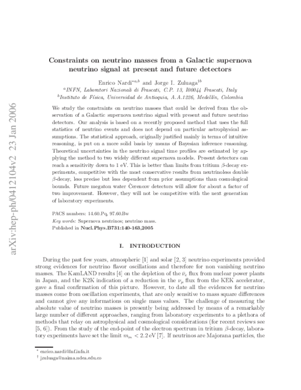
 Jorge Callejas