Lexi2: Lexicase Selection with Lexicographic Parsimony Pressure Allan de Lima Samuel Carvalho Douglas Mota Dias∗ University of Limerick Limerick, Ireland Allan.DeLima@ul.ie Limerick Institute of Technology Limerick, Ireland samuel.carvalho@lit.ie Rio de Janeiro State University Rio de Janeiro, Brazil douglas.dias@uerj.br douglas.motadias@ul.ie Enrique Naredo Joseph P. Sullivan Conor Ryan University of Limerick Limerick, Ireland Enrique.Naredo@ul.ie Limerick Institute of Technology Limerick, Ireland joe.sullivan@lit.ie University of Limerick Limerick, Ireland Conor.Ryan@ul.ie ABSTRACT 1 Bloat, a well-known phenomenon in Evolutionary Computation, often slows down evolution and complicates the task of interpreting the results. We propose Lexi2 , a new selection and bloat-control method, which extends the popular lexicase selection method, by including a tie-breaking step which considers attributes related to the size of the individuals. This new step applies lexicographic parsimony pressure during the selection process and is able to reduce the number of random choices performed by lexicase selection (which happen when more than a single individual correctly solve the selected training cases). Furthermore, we propose a new Grammatical Evolution-specific, low-cost diversity metric based on the grammar mapping modulus operations remainders, which we then utilise with Lexi2 . We address four distinct problems, and the results show that Lexi2 is able to reduce significantly the length, the number of nodes and the depth for all problems, to maintain a high level of diversity in three of them, and to significantly improve the fitness score in two of them. In no case does it adversely impact the fitness. Evolutionary Algorithms (EAs), such as Genetic Programming (GP) [12] and Grammatical Evolution (GE) [21], are a group of algorithms inspired by Darwin’s theory of evolution by natural selection, in which we evolve a population of solutions following the principle of survival of the fittest and applying some genetic operators, such as crossover and mutation. Since methods like GP or GE evolve solutions using a variablelength representation, a possible and undesirable effect is the occurrence of sharp growth of these solutions [18]. Populations experiencing such a growth rarely enjoy a corresponding improvement in fitness. This growth without a relevant increase in fitness is known as bloat [20]. Indeed, there are some forms of GP, such as Cartesian Genetic Programming, in which bloat is not a problem [25], but for many others, bloat is a naturally occurring issue. As a consequence of this phenomenon, the evolutionary process can slow down because bigger solutions usually take more time to be evaluated. Moreover, the interpretability can be difficult, and even the generalisation ability can be limited because more complex solutions can result in overfitting of the training set. Lexicographic parsimony pressure is a method introduced for controlling the bloat of GP trees which consists of choosing the smallest option when two or more solutions present identical fitness. It was tested on different problem domains, maintaining similar results regarding the fitness score, while reducing the tree sizes significantly [14]. Lexicase selection is mostly used as a parent selection method, and it has been shown to give significantly better results when compared to other selection methods, such as roulette and tournament, albeit at a cost of speed. This method consists of selecting individuals by filtering a pool of them, which starts with the entire population, and step by step, each training case is examined in random order, while the filtering process filters individuals according to the performance on each training case [24]. In an ideal situation, lexicase selection checks training cases until a single candidate remains in the pool of individuals. However, if more than one individual remains after filtering with all training cases, the selection is made randomly within the remaining individuals. In this paper, we propose Lexi2 , a new selection method, which inserts lexicographic parsimony pressure as a step of lexicase selection. The concept of including non-error metrics inside lexicase CCS CONCEPTS · Computing methodologies → Genetic programming; Supervised learning; Discrete space search. KEYWORDS lexicase selection, lexicographic parsimony pressure, grammatical evolution ACM Reference Format: Allan de Lima, Samuel Carvalho, Douglas Mota Dias, Enrique Naredo, Joseph P. Sullivan, and Conor Ryan. 2022. Lexi2 : Lexicase Selection with Lexicographic Parsimony Pressure. In Genetic and Evolutionary Computation Conference (GECCO ’22), July 9ś13, 2022, Boston, MA, USA. ACM, New York, NY, USA, 9 pages. https://doi.org/10.1145/3512290.3528803 ∗ Also with University of Limerick. This work is licensed under a Creative Commons Attribution International 4.0 License. GECCO ’22, July 9ś13, 2022, Boston, MA, USA © 2022 Copyright held by the owner/author(s). ACM ISBN 978-1-4503-9237-2/22/07. https://doi.org/10.1145/3512290.3528803 929 INTRODUCTION GECCO ’22, July 9–13, 2022, Boston, MA, USA A. de Lima, et al. selection was investigated once in a work that combines modularity metrics with error values to guide the evolution of modular solutions [23]. With our proposal, we aim to reduce the bloat of GE individuals, and simultaneously perform fewer random choices with lexicase when selecting parents. Since individuals in GE can be represented as trees, a straightforward metric for individuals’ size is their number of nodes, i.e., the fewer nodes an individual has, the smaller it is. Therefore, the number of nodes is our first choice as a tie-breaking criterion in this work. At the same time, alternative metrics linked to individuals’ size, such as tree depth and the number of genotypic used codons, are also investigated. 2 (1) Initialise: (a) Put the entire population in a pool of candidates (b) Put all training cases in a list of cases in random order (2) Loop: (a) Replace candidates with the individuals currently in candidates, which presented the best fitness for the first training case in cases (b) If a single individual remains in candidates, return this individual (c) Else if a single training case remains in cases, try to break the tie between the remaining individuals in candidates (i) Replace candidates with the individuals currently in candidates, which presented the best value regarding a pre-defined tie-breaking criterion (ii) If a single individual remains in candidates, return this individual (iii) Otherwise, return a random individual within the remaining individuals in candidates (d) Else eliminate the first training case in cases and re-run the Loop BACKGROUND GE is an EA method used to build programs [21][17][22]. We can represent a GE individual through its genotype, a variable-length sequence of codons (groups of eight bits), each consisting of an integer value . This genotype can be mapped to a phenotype, which is usually a more understandable representation to the user [5]. A grammar is a set of rules, each represented by a non-terminal and a set of production rules, which consists of terminals, items that can appear in the final program, and non-terminals, intermediate structures used by the production rules. The modulo operator1 is used to select production rules during the mapping process. A GE individual is considered invalid when the mapping process is not able to eliminate all non-terminals [16][15]. Lexicase selection is a method for selecting parents throughout the evolutionary process, which considers the fitness of each training case individually and in random order instead of an aggregated fitness value over the training cases. The original algorithm [24] starts with the entire population in a pool of candidates to be selected as parents, and the list of training cases is considered in random order. The first training case is checked, and only the candidates with the best fitness value in that training case remain in the pool. The subsequent training cases are checked until just a single candidate remains in the pool. When it happens, that individual is selected as a parent. But, if more than one candidate stays in the pool after all training cases have been checked, the parent is chosen randomly among the remaining candidates. This method was initially applied to modal problems [24], in which solutions must execute different actions on particular training cases. Later, its application was expanded to uncompromising problems [10], in which a solution is not allowed to accept a low performance in one training case in return for high performance in other training cases. After that, the method was tested successfully in other contexts such as program synthesis problems [8] and learning classifier systems [1]. A reason which may partially explain its success is the ability of lexicase selection to maintain higher levels of diversity for the population compared to methods that use aggregated fitness values, while still providing enough selection pressure to exploit good solutions [10][7]. 3 Listing 1: Algorithm for Lexi2 selection one picked later, which works only for sorting within those that have the same fitness in the first training case. This analogy with the lexicographic concept inspired the name łlexicasež. In this work, we propose extending this aspect to other attributes other than fitness. Therefore, since we are expanding the analogy, it inspired the name Lexi2 (reads łlexi squaredž). Listing 1 shows the algorithm of Lexi2 to select a parent, which is similar to the original lexicase algorithm [24], with the addition of a tie-breaking step. We reach this step when more than one candidate remains in the pool after checking all training cases. In this way, we filter the remaining candidates by considering a pre-defined tie-breaking criterion, expecting to pick the best candidate with this criterion. Still, if more than one has the best value, we choose randomly from them. However, we can also expand this step to use more than one criterion. In this way, if a tie still remains after a first attempt to break it, we try again by checking a different pre-defined criterion within the remaining individuals, and so on, using as many criteria as we want, until a single individual remains in the pool. Two criteria are used in this work, and we choose their ordering randomly in each attempt of filtering. It is necessary in order to avoid introducing some hierarchy within different criteria and expand the search space. In addition, since we are proposing Lexi2 to decrease bloat issues, we are measuring and addressing as tie-breaking criteria only those attributes related to the size of a GE individual, such as the number of nodes and the depth of the tree-representation of the phenotype, and the number of codons used to map the phenotype. In the original approach of lexicase selection, if we have ties at the end of the selection process, the individuals remaining in the pool have the same vector of fitness cases. Posterior works [19][9] use an optional pre-selection step before entering the loop of lexicase selection. It consists of taking individuals with completely equal vectors of fitness cases, and choosing a single one randomly to LEXI2 The lexicase method uses the lexicographic concept because the fitness of each training case is considered łlexicographicallyž [24]. It means that the fitness of a training case has priority over another 1 this executes an operation which returns the remainder of a division 930 Lexi2 : Lexicase Selection with Lexicographic Parsimony Pressure GECCO ’22, July 9–13, 2022, Boston, MA, USA keep in the pool of candidates. It results in an initial pool of unique individuals regarding fitness cases, which allows the process to escape from the loop earlier since it avoids the situation when we would have many cases remaining in the filtering process, but the remaining candidates would have the same fitness cases values. This approach significantly reduces the computational cost of lexicase selection, but has no practical effects on the results, since it does not change the probability of any individual being selected. Therefore, despite the higher computational cost, we decided not to use a pre-selection step in this work. We consider that it is easier to understand what is happening inside the lexicase loop using its original approach [24], and compare it with the Lexi2 loop, as we show in Figure 5. However, for further applications, we plan and recommend using a pre-selection step with Lexi2 as well. In this way, when taking individuals with completely equal vectors of fitness cases, we choose the smallest one instead of at random. 4 <e> ::= and(<e>,<e>) | or(<e>,<e>) | not(<e>) | if(<e>,<e>,<e>) | x[0] | x[1] | x[2] | x[3] | x[4] | x[5] | x[6] | x[7] | x[8] | x[9] | x[10] (a) 11-bit Multiplexer <e> ::= and(<e>,<e>) | or(<e>,<e>) | not(<e>) | x[0] | x[1] | x[2] | x[3] | x[4] (b) 5-bit Parity <e> ::= o1 = <log_op>; o0 = <log_op> <log_op> ::= and(<log_op>,<log_op>) | or(<log_op>,<log_op>) | not(<log_op>) | <boolean_feature> <boolean_feature> ::= x[0] | x[1] | x[2] | x[3] | x[4] | x[5] | x[6] | x[7] | x[8] | x[9] | x[10] | x[11] | x[12] | x[13] | x[14] | x[15] | x[16] | x[17] | x[18] | x[19] | x[20] REMAINDERS DIVERSITY (c) Car Evaluation Although the relationship between performance and diversity is not simple, the preservation of diversity in populations is usually considered desirable to help avoid premature convergence [3]. Due to the way in which the GE mapping process operates, individuals with different genotypes can produce similar or even identical phenotypes. This means that phenotypic diversity measurements probably give a more accurate view of the population than genotypic diversity measurements. In this work, we use two different phenotypic diversity measurements. The first, named fitness diversity, is defined as the number of different fitness values identified in the population divided by the number of possible values [11]. In classification problems, if we define the fitness score as the number of outputs correctly predicted, the number of possible fitness values will usually be the number of different samples plus one, since there is a possibility that no outputs have been correctly predicted. The second, structural diversity, is defined as the number of different program structures found in the population divided by the population size [11]. We can consider the phenotype of an individual as the structure, which would not be a trivial measure to implement in GE. However, since we use the modulo operator in the mapping process, we can consider the resulting sequence of remainders of an individual genotype during the mapping process as a representation of its phenotype. Thus, specifically for GE, we can redefine structural diversity as the number of different sequences of remainders found in the population divided by the population size. We name this measure remainders diversity, which is entirely equivalent to structural diversity, but much cheaper to calculate. 5 <e> ::= and(<e>,<e>) | or(<e>,<e>) | not(<e>) | if(<e>,<o>,<e>) | x[0] | x[1] | x[2] | x[3] | x[4] | x[5] | x[6] <o> ::= 0 | 1 | 2 | 3 | 4 | 5 | 6 | 7 | 8 | 9 (d) LED Listing 2: Grammars features. Finally, we also address the LED problem, a noisy dataset with ten classes, each referring to a digit from 0 to 9, and 7 binary features, each with a probability of 0.1 of being in error [2]. In our grammars (Listing 2), we define the function sets using the same approach as Koza [12] for the Boolean problems. This means using the operators AND, OR and NOT for both problems and the IF function for the 11-bit Multiplexer. This function is the common LISP function which has three arguments and executes the IF-THEN-ELSE operation. In addition, since the remaining problems have only binary inputs, we employ the same function sets. However, our idea is to analyse the performance of Lexi2 with not only various problems, but also distinct grammars, so we try different structures. In the LED problem, we expect that a reasonable individual has integer outcomes, but its grammar also allows individuals with Boolean outcomes. When it happens, these individuals can correctly predict only the classes 0 or 1, resulting in poor performance. Then, we let GE identify this issue, and Lexi2 reduce the size of the solutions. Regarding the Car Evaluation problem, the grammar provides the creation of individuals with two binary outcomes, which we use to predict the four classes of this problem. We use the whole dataset as the training set for our Boolean problems, since we aim to find individuals with perfect score. On the other hand, for the Car Evaluation and the LED problems, we split the samples into training (70%) and test sets (30%), doing a different split in each run in order to build a better statistical analysis. We can see in Table 1 the hyperparameters used in all experiments. The choice of these parameters was based on a small set of initial runs and, for Boolean problems, population size was set to a sufficient value to find individuals with a perfect score in some EXPERIMENTAL SETUP We address the key problems from a recent work [1] which studied the effects of lexicase parent selection on classification problems. Firstly, we use the 11-bit Multiplexer and the 5-bit Parity, two Boolean problems traditionally used as benchmarks in evolutionary algorithms. Secondly, we pick the Car Evaluation problem, a strongly unbalanced dataset with four classes and six categorical features, in which we used one-hot encoding to provide 21 binary 931 GECCO ’22, July 9–13, 2022, Boston, MA, USA A. de Lima, et al. 0.5 runs. In the table, the population size values refer to the multiplexer, parity, Car Evaluation and LED problems, respectively. Lexicase Lexi2 - nodes Lexi2 - depth Lexi2 - used codons Lexi2 - nodes and depth Lexi2 - used codons and depth Lexi2 - used codons and nodes 0.3 0.2 Training fitness 0.4 Table 1: Experimental hyperparameters Parameter type Parameter value Number of runs 30 Number of generations 200 Population size 500/2000/1000/1000 Elitism ratio 0.01 Mutation method Codon-based integer flip [6] Mutation probability 0.01 Crossover method Variable one-point [6] Crossover probability 0.8 Initialisation method PI Grow [4] 0.1 0 50 100 Generations 150 200 (a) 11-bit Multiplexer 0.5 We define as fitness function the mean absolute error (MAE). Since we evolve classifiers for all problems, this measure represents the rate of outputs wrongly predicted, and therefore, we want to minimise the fitness score and give invalid individuals the worst fitness value possible. Regarding the training cases, each one has only two possible outcomes: 1, if it is correctly predicted, and 0 otherwise. We run experiments with Lexi2 using each time the number of nodes, the number of used codons or the depth as a tie-breaker, and also every combination of two of them. Furthermore, we run experiments with lexicase in order to compare the results. 6 0.3 0.2 Training fitness 0.4 0.1 0 RESULTS AND DISCUSSION 50 100 Generations 200 (b) 5-bit Parity We start this section by summarising graphically the results of lexicase selection and Lexi2 with six distinct combinations of tiebreaking criteria, with all graphs showing the average between 30 runs, and in the end, we present a statistical analysis to support our results. Figure 1: Average fitness of the best individual across generations Table 2: Number of successful runs in the 11-bit Multiplexer and 5-bit Parity problems 6.1 Fitness Figure 1 shows the fitness of the best individual across generations for the Boolean problems, while Table 2 shows the number of successful runs2 . In the multiplexer problem, we can see that all approaches using Lexi2 converge to a perfect score faster than those using lexicase selection. This happens because all Lexi2 approaches achieved 29 or 30 successful runs, while lexicase achieved 24 successful runs. On the other hand, in the 5-bit Parity problem we do not have a clear superiority of Lexi2 , but the approach using the number of nodes and the number of used codons as tie-breaking criteria converges to the smallest value, achieving 12 successful runs, while the approach with lexicase achieves eight successful runs. For the Car Evaluation and LED problems, unlike when using Boolean datasets, the idea is to find solutions with the ability to generalise the training set. Therefore, the fitness result that matters is measured on a test set, and we do this only with the best individual of each run. Figure 2 shows these results as box plots. In the Car Evaluation problem, the results for four set-ups of Lexi2 present a slightly smaller average than the results using lexicase selection. 2 runs 150 Lexicase selection Lexi2 (nodes) Lexi2 (depth) Lexi2 (used codons) Lexi2 (nodes and depth) Lexi2 (used codons and depth) Lexi2 (used codons and nodes) Successful runs (out of 30) 11-bit Multipler 5-bit Parity 24 8 29 9 29 9 30 10 30 7 29 7 29 12 The best one is the approach using the number of used codons as the tie-breaking criterion. In contrast, four set-ups of Lexi2 present clearly better results for the LED problem, especially the approach using the number of nodes and the depth as tie-breaking criteria. 6.2 Bloat Figure 3 shows our most important results, since a key aim of this work is to reduce the bloat in GE individuals. The graphs present the average number of nodes in the population across the generations. Lexi2 is able to reduce the bloat in every problem, no that found a solution, which satisfies all test cases in a Boolean problem 932 Lexi2 : Lexicase Selection with Lexicographic Parsimony Pressure GECCO ’22, July 9–13, 2022, Boston, MA, USA (b) LED (a) Car Evaluation Figure 2: Box plots with the test fitness score achieved by the best individual of each run 1,000 1,000 1,000 800 800 800 800 600 600 600 400 400 400 200 200 200 600 400 Number of nodes 1,000 200 0 50 100 150 Generations (a) 11-bit Multiplexer 200 0 50 100 150 200 Generations 0 50 100 150 200 0 Lexicase Lexi2 - nodes Lexi2 - depth Lexi2 - used codons Lexi2 - nodes and depth Lexi2 - used codons and depth Lexi2 - used codons and nodes 50 Generations (b) 5-bit Parity (c) Car Evaluation 100 150 200 Generations (d) LED Figure 3: Average number of nodes across generations matter which tie-breaking criteria are being used. The results are especially good for the multiplexer problem, but even for the Car Evaluation problem, which presented the least impressive results, we can see clearly a decrease when using Lexi2 in comparison with the results from lexicase selection. we can observe that the convergence value is smaller when using Lexi2 than using lexicase for all problems. 6.4 Selection process analysis We can see the average number of individuals being selected in each step of lexicase and Lexi2 in Figure 5. This is an interesting analysis for this work because it shows in detail what is happening inside the selection process over generations. Firstly, we need to highlight that the sum of each step for each method is equal to the total number of selected individuals, which means the population size minus the elitism size. Lexicase has only two steps: selection by error, which means that only one individual remains in the pool of candidates after all training cases have been checked, and random selection, which means that the previous step ended in a tie. Then, the number of individuals being selected by lexicase is equal to the sum of these two quantities. On the other hand, Lexi2 has one or more tie-breaking steps between those, and then the number of individuals being selected is equal to the sum of these three or more steps. For instance, in Figure 5 we have a step related to selection by error, two tie-breaking steps, and also random selection, in a total of four steps for Lexi2 . This figure shows the results of the approach using the number of nodes and the depth as tie-breakers, but the results are similar to when using other approaches. Moreover, in these graphs, we show the number of individuals being selected by tiebreaker 1 and by tiebreaker 2, rather the number of nodes or the depth, because the choice of which criterion is being considered first is made randomly. 6.3 Invalid individuals Although reducing the occurrence of invalid individuals during a run was not a specific aim of this work, we noted that our experiments did precisely this, most probably as a consequence of the reduction in the individuals’ size, since smaller individuals are less likely to turn into invalid solutions. Figure 4 shows the decimal logarithm of 𝜈 across generations, where 𝜈 is the average number of invalid individuals in each generation, except when this average is zero. We choose this approach to show these results because we have a too sharp peak of invalid individuals in the second generation. We have no invalid individuals in the first generation, since we are using Position Independent Grow [4] as the initialisation method, in which complete individuals are generated. Another aspect of each initial individual is that the genome length is 50% longer than the number of used codons [16]. However, this tail is generated randomly, and then, after the parents are selected in the first generation, crossover and mutation operations create a huge number of invalid individuals, and the peak of each graph is right in the second generation, because of the randomness of the tails. Over time, the number of invalid individuals decreases sharply, and 933 GECCO ’22, July 9–13, 2022, Boston, MA, USA 3 A. de Lima, et al. 3 3 2 2 2 1 1 1 Lexicase Lexi2 - nodes Lexi2 - depth Lexi2 - used codons Lexi2 - nodes and depth Lexi2 - used codons and depth Lexi2 - used codons and nodes log(𝜈) 2 3 1 0 50 100 150 200 0 50 100 150 200 0 50 100 150 200 0 50 100 Generations Generations Generations Generations (a) 11-bit Multiplexer (b) 5-bit Parity (c) Car Evaluation (d) LED 150 200 Figure 4: Decimal logarithm of the average number of invalid individuals (except when equal to zero) across generations 500 300 200 100 0 Number of individuals 400 2,000 1,500 Lexicase (error) Lexicase (random) Lexi2 (error) Lexi2 (tiebreaker 1) Lexi2 (tiebreaker 2) Lexi2 (random) 50 100 150 Generations (a) 11-bit Multiplexer 1,000 1,000 800 800 600 600 400 400 200 200 1,000 500 200 0 50 100 150 200 Generations 0 50 100 150 Generations (b) 5-bit Parity (c) Car Evaluation Figure 5: Average number of individuals being selected in each step of lexicase and the depth as tie-breakers The graphs related to the multiplexer and parity problems are similar, but while the multiplexer results are clearly converged, the parity results are still changing, since it is a harder problem. Despite that, both graphs in both approaches start with the number of selections by error being almost equal to the total number of selections, and then converging to zero. The approach using Lexi2 converges slightly faster as it happens in the graph related to the training fitness (Figure 1). In these problems, the number of individuals selected by error is related to the fitness score, because when one individual achieves a perfect score, it will be selected as a parent every time in the next generation. Then, the evolutionary process performs crossover and mutation operations using just this single parent, generating a new population, in which we expect to find distinct individuals with a perfect score. When using lexicase, the selection process selects randomly within these individuals from the next generation until the end, but using Lexi2 it tries to break the tie before selecting randomly, and thus, the evolution advances in order to find better solutions. In short, there are no more selections by error after we have more than one individual with a perfect score in the population, and then the random selection becomes predominant, with some individuals being selected in the tie-breakings, when using Lexi2 . Alternatively, in the Car Evaluation and LED problems, the selection by error is predominant throughout generations. It is especially evident for the Car Evaluation problem, in which the convergence value of the number of selections by error is approximately 90% of the total number. It means that the number of random selections is small even when using lexicase. Furthermore, it explains why the differences between the results using lexicase and Lexi2 are small Lexi2 200 0 50 100 150 200 Generations (d) LED when using the number of nodes and in Figure 2, and even in Figure 3. However, despite the selections by error being dominant across generations for the LED problem, the number of random choices is approximately 40% of the total number when using lexicase. Lexi2 is able to reduce this percentage to less than 20%, but it does not necessarily mean that tie-breakers make all the remaining choices. Surprisingly, Lexi2 increases significantly the number of individuals selected by error in this problem. Surely, it has some relation with the improvement in the test fitness shown in Figure 2. We know that smaller individuals are less likely to overfit, which explains the decrease of the error score for the LED problem, but it does not justify the reduction of the error for the multiplexer and parity problems, where we need to overfit the training set. We hypothesise that smaller individuals are closer to the ideal size of a perfect individual, then the evolutionary process when using Lexi2 traverses in a sense the search space in a more limited dimensionality, and therefore is able to find better solutions. Moreover, we could say regarding the LED problem that this limited exploration of the search space neglects to some extent the noise of the dataset, and the LED problem has a hard dataset with too much noise. 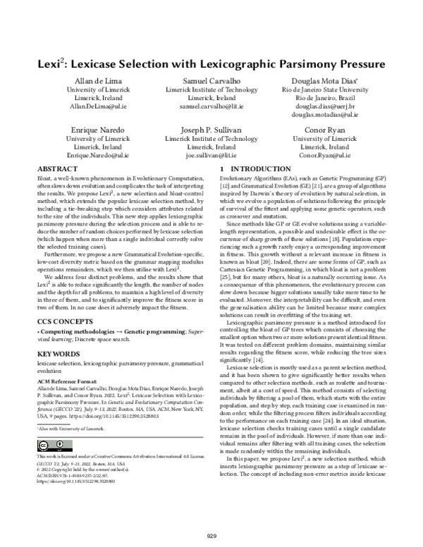6.5 Diversity An important aspect of lexicase selection is that it is an excellent method for maintaining a high level of diversity in a population [8]. Thus, one of the expectations of this work is to maintain at least the same level of diversity when using Lexi2 . Figure 6 shows the fitness diversity, and we can see that lexicase selection is better at maintaining diversity in the multiplexer problem, but that Lexi2 is 934 Lexi2 : Lexicase Selection with Lexicographic Parsimony Pressure 0.4 0.2 Fitness diversity 0.6 0 50 100 150 200 GECCO ’22, July 9–13, 2022, Boston, MA, USA 0.6 0.6 0.6 0.4 0.4 0.4 0.2 0.2 0.2 0 50 Generations 100 150 0 200 50 Generations 150 200 0 50 Generations (b) 5-bit Parity (a) 11-bit Multiplexer 100 Lexicase Lexi2 - nodes Lexi2 - depth Lexi2 - used codons Lexi2 - nodes and depth Lexi2 - used codons and depth Lexi2 - used codons and nodes 100 150 200 Generations (c) Car Evaluation (d) LED Figure 6: Average fitness diversity 1 1 1 0.8 0.8 0.8 0.8 0.6 0.6 0.6 0.4 0.4 0.4 0.2 0.2 0.2 0.6 0.4 0.2 0 Remainders diversity 1 50 100 150 200 Generations (a) 11-bit Multiplexer 0 50 100 150 200 0 50 Generations 100 150 Generations (b) 5-bit Parity (c) Car Evaluation 200 0 Lexicase Lexi2 - nodes Lexi2 - depth Lexi2 - used codons Lexi2 - nodes and depth Lexi2 - used codons and depth Lexi2 - used codons and nodes 50 100 150 200 Generations (d) LED Figure 7: Average remainders diversity slightly better for the other three problems. We can make almost identical observations in Figure 7, which shows the remainders diversity. In both the parity and LED problems the results are so similar that it is not possible to separate lexicase and Lexi2 . Note that the conclusions derived for diversity are the same regardless of which diversity measurement is used, which gives us confidence in our proposed remainders diversity, which is easy to understand and inexpensive to run. statistical significance in this stricter scenario are highlighted with an asterisk. Also, whenever Lexi2 did not outperform Lexicase an italic font was used in the tables. In the multiplexer problem, the best fitness has improved in all scenarios, with five of them statistically significant before the Bonferroni correction. Meanwhile, all the size-related metrics have presented a drastic and significant improvement in all scenarios, with many-fold decreases. For the parity problem, while the best fitness presents better averages in five of the cases, none of them were significantly better. However, once again, all the size-related metrics have shown a statistically significant improvement, with a single loss of significance after correction. For the Car Evaluation problem, test fitness was not significantly changed when compared to Lexicase. Meanwhile, size metrics presented smaller averages in all cases except two, but not all of them with statistical significance, especially after the Bonferroni correction. In the LED problem, test fitness has improved in all scenarios where Lexi2 was used, with a statistically significant improvement in four of the six strategies (three with Bonferroni). All three sizerelated metrics analysed have presented a significant reduction, with resulting individuals notably smaller than the ones seen in Lexicase selection. 6.6 Statistical Analysis Given the various metrics and different tie-break strategies used in the Lexi2 experiments presented on this paper, a statistical analysis was performed to investigate the significance of the findings. The expected outcome was that Lexi2 would be able to consistently improve size-related metrics (such as length, number of nodes and depth of the individuals) without damaging overall fitness metrics when compared to the original lexicase method. Tables 3, 4, 5 and 6 present the results from these analyses, where statistically significant differences are underlined for a clearer interpretation. Pairwise comparisons between each Lexi2 tie-break strategy and lexicase selection were conducted, and the tables represent the end-result for each of the metrics, i.e., at the final generation of each of the runs on a given problem. The t-student test with a p-value threshold of 0.05 for rejection of the null hypothesis (no difference between the metrics) was used for the comparisons, after the Shapiro-Wilk test has indicated the normality of the data under analysis. In addition, even though only standalone pairwise comparisons were performed, a stricter analysis using the Bonferroni correction with a factor of 6 within each metric was also conducted, with similar results. The corrected p-value was set to 0.00833, and the metrics that have lost 7 CONCLUSION In this paper, we carried out an improvement in the lexicase selection technique by applying parsimony pressure inside the selection process, which is able to perform fewer random choices when selecting parents. Our first target was to reduce the bloat, which 935 GECCO ’22, July 9–13, 2022, Boston, MA, USA A. de Lima, et al. Table 3: 11-bit Multiplexer: mean metrics for each approach and p-values between lexicase selection and each strategy of Lexi2 Fitness Length Nodes Depth Lexicase Average 8.85E-03 2.16E+03 4.54E+02 2.23E+01 nodes p-value Average 2.21E-02* 2.60E-04 2.16E-06 3.47E+02 1.06E-13 5.49E+01 4.13E-17 7.03E+00 depth p-value Average 1.85E-02* 1.63E-05 6.48E-05 5.37E+02 2.67E-12 8.91E+01 2.60E-15 8.42E+00 used codons p-value Average 1.83E-02* 0.00E+00 1.05E-06 3.05E+02 2.20E-14 4.68E+01 5.26E-18 6.71E+00 Lexi2 nodes and depth p-value Average 1.83E-02* 0.00E+00 1.31E-06 3.15E+02 1.85E-14 4.52E+01 2.30E-18 6.56E+00 used codons and depth p-value Average 1.12E-01 2.08E-03 3.58E+02 2.18E-06 5.31E+01 4.95E-14 7.17E+00 2.63E-17 used codons and nodes p-value Average 0.00E+00 1.83E-02* 2.89E+02 8.73E-07 4.53E+01 1.86E-14 6.74E+00 4.26E-18 Table 4: 5-bit Parity: mean metrics for each approach and p-values between lexicase selection and each strategy of Lexi2 Fitness Length Nodes Depth Lexicase Average 4.79E-02 4.10E+03 5.39E+02 2.77E+01 nodes p-value Average 4.50E-01 4.06E-02 7.34E-04 2.73E+03 6.85E-08 3.45E+02 3.83E-07 2.28E+01 depth p-value Average 3.98E-01 3.96E-02 2.02E-03 2.92E+03 3.05E-02* 4.49E+02 4.49E-05 2.37E+01 used codons p-value Average 3.92E-01 3.96E-02 4.07E-05 2.38E+03 1.36E-06 3.50E+02 3.74E-05 2.33E+01 Lexi2 nodes and depth p-value Average 1.00E+00 4.79E-02 3.16E-05 2.44E+03 1.31E-05 3.84E+02 2.41E-08 2.28E+01 used codons and depth p-value Average 7.41E-01 4.48E-02 2.71E-04 2.65E+03 1.04E-05 3.74E+02 1.41E-07 2.28E+01 used codons and nodes p-value Average 4.42E-01 3.96E-02 5.89E-05 2.51E+03 2.89E-08 3.38E+02 2.51E-08 2.26E+01 Table 5: Car Evaluation: mean metrics for each approach and p-values between lexicase selection and each strategy of Lexi2 Fitness Length Nodes Depth Lexicase Average 1.02E-01 2.28E+03 8.50E+02 4.14E+01 nodes p-value Average 8.70E-01 1.01E-01 7.27E-01 2.38E+03 2.98E-02* 7.44E+02 4.62E-03 3.90E+01 depth p-value Average 8.20E-01 1.01E-01 2.27E-01 2.05E+03 3.32E-01 8.00E+02 1.92E-04 3.79E+01 used codons p-value Average 4.95E-01 9.85E-02 6.49E-01 2.17E+03 5.11E-03 7.16E+02 1.21E-02* 3.88E+01 Lexi2 nodes and depth p-value Average 5.42E-01 1.05E-01 3.87E-01 2.11E+03 6.76E-01 8.22E+02 2.50E-02* 3.97E+01 used codons and depth p-value Average 6.49E-01 1.04E-01 7.87E-01 2.22E+03 9.90E-02 7.69E+02 3.30E-03 3.87E+01 used codons and nodes p-value Average 8.99E-01 1.01E-01 9.13E-01 2.31E+03 4.17E-02* 7.58E+02 7.01E-03 3.91E+01 Table 6: LED: mean metrics for each approach and p-values between lexicase selection and each strategy of Lexi2 Fitness Length Nodes Depth Lexicase Average 3.49E-01 3.48E+03 3.43E+02 2.64E+01 nodes p-value Average 3.45E-03 3.12E-01 2.77E-10 1.07E+03 9.77E-08 2.45E+02 2.99E-13 2.14E+01 depth p-value Average 2.02E-02* 3.19E-01 4.68E-10 1.11E+03 2.51E-09 2.45E+02 3.11E-14 2.14E+01 used codons p-value Average 5.38E-02 3.22E-01 2.51E-09 1.19E+03 4.90E-08 2.51E+02 1.12E-10 2.20E+01 Lexi2 nodes and depth p-value Average 1.54E-03 3.07E-01 1.59E-10 1.04E+03 3.44E-06 2.60E+02 1.19E-10 2.15E+01 used codons and depth p-value Average 3.13E-01 6.25E-03 1.08E+03 1.06E-09 2.49E+02 7.99E-09 2.14E+01 8.03E-14 used codons and nodes p-value Average 7.25E-02 3.25E-01 9.52E+02 5.42E-11 2.35E+02 5.79E-09 2.07E+01 6.84E-14 Lexi2 addressing attributes that are not related to the size of the individuals, such as considering parsimonious power consumption when aiming at evolving low-power digital circuits. Moreover, we developed Lexi2 using GE, but this is not a GE-specific method, and it can be easily applied to many forms of GP. Another future work is to apply Lexi2 to regression problems. Firstly, we need to define another way to specify what is a tie, since the fitness space is not discrete. Following the same approach as Epsilon-Lexicase selection [13], where individuals within a certain threshold of the target are considered to be successful, we can choose the smallest one among these individuals. significantly happened for all problems addressed when considering the length of the genome, the number of nodes and the depth in comparison with traditional lexicase. We achieved this while maintaining at least a similar fitness score, and, for three of the problems examined, Lexi2 produced better results. We believe that smaller individuals present a better generalisation ability due to their simplicity. The statistical analysis of the experiments presented in this paper has validated the rationale behind the development of the Lexi2 method: it is capable of consistently reducing the size of the generated individuals while maintaining the same overall fitness results obtained with Lexicase. Lexi2 is also able to maintain a high level of diversity in the population in three problems addressed, and this was measured with two distinct diversity measurements, one of which, remainders diversity, is a new GE-specific way to measure diversity. In future work, we plan to compare this new measure with a more informative phenotypic diversity like behavioural diversity. Although this work is related to the bloat issue, we believe that we can implement this technique addressing any other attribute as a tie-breaker. Thus, as another future work, we plan to apply 8 ACKNOWLEDGMENTS This publication has emanated from research conducted with the financial support of Science Foundation Ireland under Grant number 16/IA/4605. The third author is also financed by the Coordenação de Aperfeiçoamento de Pessoal de Nível Superior - Brazil (CAPES), Finance Code 001, and the Fundação de Amparo à Pesquisa do Estado do Rio de Janeiro (FAPERJ). Open Access funding provided by the IRel Consortium. 936 Lexi2 : Lexicase Selection with Lexicographic Parsimony Pressure GECCO ’22, July 9–13, 2022, Boston, MA, USA REFERENCES [20] Riccardo Poli, William B. Langdon, and Nicholas Freitag McPhee. 2008. A field guide to genetic programming. Published via http://lulu.com and freely available at http://www.gp-field-guide.org.uk, UK. http://www.gp-fieldguide.org.uk (With contributions by J. R. Koza). [21] Conor Ryan, J. Collins, and Michael O’Neill. 1998. Grammatical Evolution: Evolving Programs for an Arbitrary Language.. In Lecture Notes in Computer Science. Springer, Berlin, Heidelberg, 83ś96. https://doi.org/10.1007/BFb0055930 [22] Conor Ryan, Michael O’Neill, and J. J. Collins (Eds.). 2018. Handbook of Grammatical Evolution. Springer, Boston, MA. https://doi.org/10.1007/978-3-319-78717-6 [23] Anil Kumar Saini and Lee Spector. 2019. Using Modularity Metrics as Design Features to Guide Evolution in Genetic Programming. Springer, 165ś180. [24] Lee Spector. 2012. Assessment of Problem Modality by Differential Performance of Lexicase Selection in Genetic Programming: A Preliminary Report. In Proceedings of the 14th Annual Conference Companion on Genetic and Evolutionary Computation (Philadelphia, Pennsylvania, USA) (GECCO ’12). Association for Computing Machinery, New York, NY, USA, 401ś408. https: //doi.org/10.1145/2330784.2330846 [25] Andrew Turner and Julian Miller. 2014. Cartesian Genetic Programming: Why No Bloat?. In 17th European Conference on Genetic Programming (LNCS, Vol. 8599), Miguel Nicolau, Krzysztof Krawiec, Malcolm I. Heywood, Mauro Castelli, Pablo Garcia-Sanchez, Juan J. Merelo, Victor M. Rivas Santos, and Kevin Sim (Eds.). Springer, Granada, Spain, 222ś233. https://doi.org/10.1007/978-3-662-443033_19 [1] Sneha Aenugu and Lee Spector. 2019. Lexicase Selection in Learning Classifier Systems. In Proceedings of the Genetic and Evolutionary Computation Conference (Prague, Czech Republic) (GECCO ’19). Association for Computing Machinery, New York, NY, USA, 356ś364. https://doi.org/10.1145/3321707.3321828 [2] L Breiman. 1984. Classification and regression trees. CRC press, Boca Raton, Florida. 47ś49 pages. [3] Edmund Burke, Steven Gustafson, and Graham Kendall. 2002. A Survey and Analysis of Diversity Measures in Genetic Programming. In Proceedings of the 4th Annual Conference on Genetic and Evolutionary Computation (New York City, New York) (GECCO’02). Morgan Kaufmann Publishers Inc., San Francisco, CA, USA, 716ś723. [4] David Fagan, Michael Fenton, and Michael O’Neill. 2016. Exploring position independent initialisation in grammatical evolution. In 2016 IEEE Congress on Evolutionary Computation (CEC). IEEE, Vancouver, Canada, 5060ś5067. https: //doi.org/10.1109/CEC.2016.7748331 [5] David Fagan, Michael O’Neill, Edgar Galvan-Lopez, Anthony Brabazon, and Sean McGarraghy. 2010. An Analysis of Genotype-Phenotype Maps in Grammatical Evolution. In Proceedings of the 13th European Conference on Genetic Programming, EuroGP 2010 (LNCS, Vol. 6021), Anna Isabel Esparcia-Alcazar, Aniko Ekart, Sara Silva, Stephen Dignum, and A. Sima Uyar (Eds.). Springer, Istanbul, 62ś73. https: //doi.org/10.1007/978-3-642-12148-7_6 [6] Michael Fenton, James McDermott, David Fagan, Stefan Forstenlechner, Erik Hemberg, and Michael O’Neill. 2017. PonyGE2: Grammatical Evolution in Python. In Proceedings of the Genetic and Evolutionary Computation Conference Companion (GECCO ’17). ACM, Berlin, Germany, 1194ś1201. https://doi.org/10.1145/3067695. 3082469 [7] Thomas Helmuth, Nicholas Freitag McPhee, and Lee Spector. 2016. Effects of Lexicase and Tournament Selection on Diversity Recovery and Maintenance. In Proceedings of the 2016 on Genetic and Evolutionary Computation Conference Companion (Denver, Colorado, USA) (GECCO ’16 Companion). Association for Computing Machinery, New York, NY, USA, 983ś990. https://doi.org/10.1145/ 2908961.2931657 [8] Thomas Helmuth, Nicholas Freitag McPhee, and Lee Spector. 2016. Lexicase Selection for Program Synthesis: A Diversity Analysis. Springer International Publishing, Cham, 151ś167. https://doi.org/10.1007/978-3-319-34223-8_9 [9] Thomas Helmuth, Edward Pantridge, and Lee Spector. 2020. On the importance of specialists for lexicase selection. Genetic Programming and Evolvable Machines 21, 3 (Sept. 2020), 349ś373. https://doi.org/10.1007/s10710-020-09377-2 Special Issue: Highlights of Genetic Programming 2019 Events. [10] Thomas Helmuth, Lee Spector, and James Matheson. 2014. Solving Uncompromising Problems With Lexicase Selection. IEEE Transactions on Evolutionary Computation 19 (01 2014), 1ś1. https://doi.org/10.1109/TEVC.2014.2362729 [11] David Jackson. 2010. Promoting Phenotypic Diversity in Genetic Programming. In PPSN 2010 11th International Conference on Parallel Problem Solving From Nature (Lecture Notes in Computer Science, Vol. 6239), Robert Schaefer, Carlos Cotta, Joanna Kolodziej, and Guenter Rudolph (Eds.). Springer, Krakow, Poland, 472ś481. https://doi.org/10.1007/978-3-642-15871-1_48 [12] John R. Koza. 1992. Genetic Programming - On the Programming of Computers by Means of Natural Selection. MIT Press, Boston, USA. IśXVIII, 1ś419 pages. [13] William La Cava, Lee Spector, and Kourosh Danai. 2016. Epsilon-lexicase Selection for Regression. In GECCO ’16: Proceedings of the 2016 Annual Conference on Genetic and Evolutionary Computation, Tobias Friedrich (Ed.). ACM, Denver, USA, 741ś748. https://doi.org/10.1145/2908812.2908898 [14] Sean Luke and Liviu Panait. 2002. Lexicographic Parsimony Pressure. In Proceedings of the 4th Annual Conference on Genetic and Evolutionary Computation (New York City, New York) (GECCO’02). Morgan Kaufmann Publishers Inc., San Francisco, CA, USA, 829ś836. [15] Miguel Nicolau. 2017. Understanding grammatical evolution: initialisation. Genetic Programming and Evolvable Machines 18 (12 2017), 467ś. https://doi.org/10. 1007/s10710-017-9309-9 [16] Miguel Nicolau, Michael O’Neill, and Anthony Brabazon. 2012. Termination in Grammatical Evolution: grammar design, wrapping, and tails. In 2012 IEEE Congress on Evolutionary Computation, CEC 2012. IEEE, Brisbane, Australia, 1ś8. https://doi.org/10.1109/CEC.2012.6256563 [17] Michael O’Neill and Conor Ryan. 2003. Grammatical Evolution: Evolutionary Automatic Programming in an Arbitrary Language. Vol. 4. Springer, Boston, MA. https://doi.org/10.1007/978-1-4615-0447-4 [18] Michael O’Neill, Conor Ryan, Maarten Keijzer, and Mike Cattolico. 2003. Crossover in Grammatical Evolution. Genetic Programming and Evolvable Machines 4, 1 (March 2003), 67ś93. [19] Edward R. Pantridge, Thomas Helmuth, Nicholas Freitag McPhee, and Lee Spector. 2018. Specialization and elitism in lexicase and tournament selection. In Proceedings of the Genetic and Evolutionary Computation Conference Companion, GECCO 2018, Kyoto, Japan, July 15-19, 2018, Hernán E. Aguirre and Keiki Takadama (Eds.). ACM, Kyoto, Japan, 1914ś1917. 937