Flegel et al. Earth, Planets and Space (2017) 69:51
DOI 10.1186/s40623-017-0633-3
Open Access
FULL PAPER
An analysis of the 2016 Hitomi breakup
event
Sven Flegel1* , James Bennett1, Michael Lachut1, Marek Möckel1 and Craig Smith2
Abstract
The breakup of Hitomi (ASTRO-H) on 26 March 2016 is analysed. Debris from the fragmentation is used to estimate
the time of the event by propagating backwards and estimating the close approach with the parent object. Based
on this method, the breakup event is predicted to have occurred at approximately 01:42 UTC on 26 March 2016. The
Gaussian variation of parameters equations based on the instantaneous orbits at the predicted time of the event are
solved to gain additional insight into the on-orbit position of Hitomi at the time of the event and to test an alternate
approach of determining the event epoch and location. A conjunction analysis is carried out between Hitomi and all
catalogued objects which were in orbit around the estimated time of the anomaly. Several debris objects have close
approaches with Hitomi; however, there is no evidence to support the breakup was caused by a catalogued object.
Debris from both of the largest fragmentation events—the Iridium 33–Cosmos 2251 conjunction in 2009 and the
intentional destruction of Fengyun 1C in 2007—is involved in close approaches with Hitomi indicating the persistent
threat these events have caused in subsequent space missions. To quantify the magnitude of a potential conjunction, the fragmentation resulting from a collision with the debris is modelled using the EVOLVE-4 breakup model. The
debris characteristics are estimated from two-line element data. This analysis is indicative of the threat to space assets
that mission planners face due to the growing debris population. The impact of the actual event to the environment
is investigated based on the debris associated with Hitomi which is currently contained in the United States Strategic
Command’s catalogue. A look at the active missions in the orbital vicinity of Hitomi reveals that the Hubble Space
Telescope is among the spacecraft which may be immediately affected by the new debris.
Keywords: Fragmentation, Debris, Spacecraft, Kessler syndrome
Background
To date, over 250 objects have broken up in Earth orbit
(Johnson et al. 2008; Flegel et al. 2011). Breakups are
especially critical whenever they occur in highly utilised
orbits such as the 800-km-altitude band or the geostationary orbit (GEO) region. A collision with an active
spacecraft may not only lead to the premature termination of the satellite’s mission, but also create additional
debris which in turn may collide with other objects. The
process wherein debris from collisions becomes the main
driver behind the creation of new debris is known as the
‘Kessler syndrome’ and may already be a reality (Kessler
*Correspondence: svenflegel@serc.org.au
1
Space Environment Research Centre (SERC) Limited, Weston Creek, ACT
2611, Australia
Full list of author information is available at the end of the article
1991; Inter-Agency Space Debris Coordination Committee—Working Group 2 2013).
A well-founded analysis of the immediate and longterm impacts of a breakup on the environment requires
knowledge not only of the amount of debris which has
been created in the event, what orbits these are on and
how long they may remain there, but also of the current
state of the environment. The largest, publicly accessible
catalogue of objects on Earth orbits is being maintained
by the United States Strategic Command (USSTRATCOM). Of the roughly 17,800 in-orbit objects currently
contained in this catalogue, 11 debris objects have been
associated with Hitomi’s breakup. As the spacecraft’s
orbit inclination was only about 30° and the orbital altitude was below 600 km, many high-accuracy groundbased sensors cannot observe or track these objects
simply because they never appear above their horizon.
© The Author(s) 2017. This article is distributed under the terms of the Creative Commons Attribution 4.0 International License
(http://creativecommons.org/licenses/by/4.0/), which permits unrestricted use, distribution, and reproduction in any medium,
provided you give appropriate credit to the original author(s) and the source, provide a link to the Creative Commons license,
and indicate if changes were made.
�Flegel et al. Earth, Planets and Space (2017) 69:51
Although it is not expected that significant debris from
the event should be missing from the catalogue, an
analysis of the recorded debris orbits is nevertheless
performed to assess whether the current understanding
of the cause of the event is in line with the number of
objects that are being tracked.
The current paper starts out with an outline of the
events leading up to the fragmentation of Hitomi as
published in media reports by Japan’s Aerospace Exploration Agency (JAXA). The time at which the satellite
broke up, the on-orbit location and the magnitude of the
event are analysed. The debris environment in the vicinity of Hitomi is then assessed by calculating close conjunctions between Hitomi and debris with known orbits.
Modelling the fragmentation of Hitomi resulting from a
collision with another object deepens the understanding
of the risks associated with such events and introduces
an alternate possible cause for the breakup. The section
also introduces another possible cause for the breakup of
Hitomi which cannot be dismissed based on the current
evidence. In the final section, the impact of the debris
created in the actual breakup of Hitomi on the debris
environment and on active spacecraft in its vicinity is
investigated.
Event description
On 31 May 2016, JAXA published a detailed report
describing events leading up to the breakup of Hitomi
(JAXA 2016). JAXA estimated the breakup to have
occurred around 1:37 UTC on March 26 by backpropagating the debris positions. This assessment is
just 5 min earlier than the epoch published by the
United States Joint Space Operations Centre (JSpOC):
1:42 UTC ±11 min. The report named four major ‘mechanisms’ which are suspected to have lead to the spacecraft being spun up by its attitude control system (ACS)
whereby both solar panels and the extensible optic bench
(EOB) are likely to have broken off: (1) the ACS indicated
the attitude state of the spacecraft as rotating when it
was not. The reaction wheel (RW) was then activated to
counteract the rotation which caused the spacecraft to
start spinning. (2) Unloading of the RW by the magnetic
torquer did not work properly. (3) Once the spacecraft
attitude situation had been determined as critical, ACS
switched to the Safe Hold mode wherein attitude thrusters were activated to return the spacecraft to a steady
attitude. After the solar arrays and the EOB had been
extended, new thruster control parameters had been
uploaded to the spacecraft to account for the changes in
centre of mass and moment of inertia. These parameters
had, however, not been tested prior to uploading and
turned out to be inaccurate. Simulations of the spacecraft
attitude with the updated ACS control parameters which
Page 2 of 13
were performed after the event showed that the thrusting would have caused the spacecraft attitude to respond
in an unexpected manner and likely increased the spacecraft spin rate further. (4) Angular rates derived from
ground-based observations of Hitomi were then fed into
finite element method simulations to test for structural
response. Within the simulations, material limits were
surpassed for both solar panels and for the EOB. The
ACS-induced spinning up of the spacecraft has therefore been established as a likely cause for the breakup of
Hitomi.
Within the current section, the event epoch and location are derived independently of the published results by
JAXA and JSpOC. The event magnitude is then assessed
based on the distribution of the orbits from the 11 catalogued debris. If the orbits suggest that a high-energy
event occurred, there should be many more debris than
the objects which have currently been identified from the
event.
Estimate of the time of the Hitomi breakup
All of the debris created from the breakup event was used
to estimate the time of the breakup by comparing their
backwards propagated orbits with that of Hitomi. The
time where the orbits are at their closest point can give
an indication of the event time. Only valid two-line elements (TLEs) (i.e., removing the erroneous Hitomi ones)
after the event were used to estimate the expected time
of the breakup event. Figure 1 (left) shows a histogram
for the time estimates for the orbit close approaches of
Hitomi and Hitomi debris objects for the period around
26 March 2016 00:00:00 UTC. Overlaid on the plot is a
normal probability density function fit to the data. The
time interval 01:00–02:00 UTC on 26 March 2016 contains the most close approach estimates. The right-hand
plot in Fig. 1 shows a histogram of the close approach
times for 01:00–02:00 UTC on 26 March 2016. Fitting a
normal distribution allows us to estimate the time of the
breakup event. This gives a mean event time as 26 March
2016 01:42 UTC (26 March 2016 10:42 JST) and expected
to fall within 01:42 ± 14 min (3σ interval).
Event location
The event position is directly linked to the event epoch.
Using SGP4 to estimate the on-orbit location of Hitomi
at the time of the event yields an argument of latitude of
u = ω + ν = 35◦ ± 52.53◦ (ω is the argument of perigee,
and ν the true anomaly).
Orbit shape and orientation in inertial space change
when a perturbing force acts on it. The manner in which
they change depends on the force’s direction and magnitude, the initial orbit, the argument of latitude and true
anomaly at which it is applied. It should be possible to
�Flegel et al. Earth, Planets and Space (2017) 69:51
Page 3 of 13
Fig. 1 Histogram and probability density function plot for the estimated breakup event times around 26 March 2016 00:00:00 UTC (left). Histogram
and probability density function plot for the estimated breakup event times during 01:00–02:00 UTC on 26 March 2016 (right)
analyse the change in osculating orbital elements around
the time of the event to determine the likely on-orbit
position of Hitomi when the event occurred. Obtaining
a solution in this manner may be helpful in confirming,
refuting or even refining the solution from the previous
close conjunction analysis.
The Gaussian form of the variation of parameters equations (Gaussian VoP) gives the time derivative of each
orbit parameter based on three orthogonal accelerations
in the RSW system [see for example Section 9.3.2 in Vallado and McClain (2013)]. For small accelerations, the
equations can be integrated by keeping all orbit parameters fixed. The resulting relations give the total change
in each parameter as the function of the change in velocity in each of the orthogonal RSW directions. Within
these equations, the orbit shape and in-plane orientation
are influenced by accelerations which are in the orbital
plane; the orientation of the orbit plane in inertial space
is only affected by accelerations normal to that plane. As
the orbit changes encountered in the case of Hitomi are
not small, the applicability of the method is first tested on
simulated fragmentation events and then applied to the
current event.
Applicability to fragmentation analyses Four main factors impact the accuracy of the method’s outcome: (1)
the method requires knowledge of the change in orbit
parameters induced during the event. As the parameters evolve differently for each object, an estimate of the
event epoch must be available beforehand. Unless this
is included as a solve-for parameter, the accuracy with
which the event epoch is known before can potentially
impact the accuracy of this method’s result. (2) The orbit
data itself usually contains non-negligible inaccuracies.
(3) The orbit parameters at the event epoch are obtained
through propagation using a tool with a given accuracy.
(4) Finally, the method relies on changes in the orbit
parameters to be small.
In the following, only the basic applicability of the
method to low-energy fragmentation events such as
the one currently being analysed along with its potential accuracy and precision is assessed. This is done by
applying the method to simulated debris clouds at the
event epoch. In this manner, uncertainties are limited to
inaccuracies at the machine level which are introduced
mainly by the transformation of the state vectors into
Keplerian elements.
Four test cases are created. The first test case T1 is
based on preliminary results from the Gaussian VoP
method applied to the breakup of Hitomi. The resulting velocity changes in RSW coordinates at the time of
the event are translated into a covariance matrix for the
velocity. The values in the matrix are increased by a factor 10 to allow for outliers to be adequately covered
within the simulation. To attain statistical significance,
1000 debris particles are created at the true anomaly
location ν = 87.21◦. These particles are all co-located
and have instantaneous velocity vectors which cover
the volume of values derived from Hitomi’s debris. The
state vectors of these particles are then transformed into
Keplerian elements and processed by the Gaussian VoP
method. The same methodology is applied to three more
test cases. The second test T2 is identical to the first test
case with the exception that the location of the event
is moved to ν = 20.00◦. The two final test cases T3 and
T4 use the same true anomaly locations as cases one
and two but assume an initial orbit eccentricity of 0.05
instead of ≈0.0009. It is found that solutions generally do
not converge, if the change in argument of perigee due to
�Flegel et al. Earth, Planets and Space (2017) 69:51
the event exceeds roughly 20°. The absolute value of the
residual error for all remaining particles is plotted against
the true anomaly of the solution in Fig. 2. It can be seen
that the true solution can be found by calculating the
mean of values with residual errors below 0.0001. Assuming a higher threshold requires manual pre-screening of
the results. For the most relevant test case T1, the resulting accuracy is worst which can be attributed to the parent orbit being near-circular and the event location near
ν = 90◦. Using the solution of particles with absolute
residual errors lower than 0.001, the mean and standard
deviation become: ν = 88.18◦ ± 2.86◦. The true value
is therefore contained in the 1-σ confidence interval, and
the mean value is accurate to within less than 1° of the
true value.
Application to Hitomi The osculating orbit at the
instances before and after the breakup is required for the
current analysis. The former is obtained by propagating
the last available TLE from before the event to the estimated event epoch 26 March 01:42 UTC using the Simplified General Perturbations 4 (SGP4) method. For each
fragment, five successive TLEs are propagated back in
time to the event epoch. The TLEs from the two objects
41438 and 41443 are omitted as they decayed within
the first month after the event. For the further analysis,
also the TLE from objects 41440, 41441 and 41446 are
disregarded as their argument of true anomaly changed
by more than 20° through the event. This is in excess of
what was established in the method testing to exceed the
requirement of parameter changes to remain small. As
Hitomi’s orbit eccentricity was on the order of only 10−3,
the argument of perigee changes very quickly. This causes
the true anomaly in the days surrounding the event to
remain within the interval [−40°, 100°]. Only those solutions from the Gaussian VoP analysis which are in this
region and have converged to an absolute solution error
of 1 × 10⁻³ are considered. The solutions from TLEs of
Page 4 of 13
the main body, which has the ‘North American Aerospace Defense Command’ (NORAD) ID 41337, do not
contribute to the overall result since their best absolute
error is at 2 × 10⁻³. The results based solely on its solutions are given independently nevertheless as its TLEs
and the results obtained from them exhibit the greatest
consistency.
The left plot within Fig. 3 shows the distribution of
results from all valid TLEs without the main body. The
evolution of true anomaly of the main body for the ±6σ
interval surrounding March 26, 01:42 UTC is obtained
by propagating the last valid TLE prior to the event forward in time. It is shown in the centre right plot in Fig. 3.
The normal probability density function (PDF) above
the true anomaly evolution represents the solution for
the predicted event epoch from the previous section.
The normal PDF derived from the simultaneous solving
of the Gaussian VoP equations for the true anomaly is
given to the right. The mean and standard deviation of
the normal distribution based on the TLE’s of all debris
are ν = 83.69◦ ± 6.23◦. The solution using only the TLE
from Hitomi’s main body is ν = 82.72◦ ± 0.08◦. Both
solutions are within a degree of one another. This is on
the order of the accuracy which can be expected of the
method when applied to the specific case of Hitomi (see
Test Case T1).
Projecting the solutions from the Gaussian VoP
method onto the time-dependent true anomaly of the
main body shows two possible locations in the ±6σ interval surrounding the estimated event epoch: one is located
at around +11 min and the other at +20 min after the
estimated event epoch. Here, only the solution closer to
the estimated event time is considered. The PDFs from
the debris close approach and from the Gaussian VoP
analyses can be combined to form a new estimate of the
event epoch. It is obtained by multiplying the normalised probability for the individual solutions at each true
Fig. 2 Solution of the Gaussian VoP method to four simulated satellite fragmentations. The grey lines indicate the true location of each event
�Flegel et al. Earth, Planets and Space (2017) 69:51
Page 5 of 13
Fig. 3 Left Histogram of results from solving of Gaussian variation of parameters equations based on the last viable TLE before the event and five
TLEs for each fragment (except for the two which decayed within a few days of the event). Right True anomaly of Hitomi predicted using SGP4
based on the last viable TLE before for the event. Normal probability density functions are given from close approach analysis for event time and
from Gaussian VoP analysis for event true anomaly. The dotted lines indicate the mean values from the normal probability density functions
anomaly/epoch. From the collected results in Table 1,
it can be seen that the mapping of the Gaussian VoP
solutions (GD, GD + CA, GA and GA + CA) onto the
time leads to asymmetric PDFs. Without knowledge of
the accuracy of the true anomaly evolution, the results
derived from the Gaussian VoP approach suggest an
event epoch of March 26, 01:52 UTC with a worst case
99.7% confidence time interval of less than 5 min which is
roughly three times lower than that of the close approach
methodology.
Several factors contribute to the credibility of the solution of the Gaussian VoP method: For one, the method
has been shown to work for simulated cases without
uncertainties. Furthermore, the mean solutions for the
event true anomaly from Hitomi’s main body and from
the debris are very close together and finally they are both
within the +3σ range of the estimated event epoch. As
the uncertainties associated with Hitomi’s true anomaly
have not been assessed here, a definitive statement as to
the absolute accuracy of the method would be premature.
In fact, such an analysis requires knowledge of the accuracy of given orbit data which is not available for TLEs.
Finally, the solutions for Δv are below 10 m/s in
radial and in-track and below 33 m/s in cross-track for
all valid solutions. This again supports JAXA’s assessment that this was not a high-energy fragmentation.
For object 41337, the solving of the Gaussian VoP equations results in �vR ≈ +7.9 m/s, �vS ≈ +0.3 m/s and
�vW ≈ −1.4 m/s which, applied at ν = 82.72◦, should
lead to the observed change in osculating orbit elements.
Event magnitude
High-energy events commonly create substantial
amounts of debris which are ejected into higher as well
as lower orbits relative to the original one. Low-energy
events typically only release a few objects and at low
relative velocities. This behaviour can be observed by
inspecting the debris clouds within the ‘History of OnOrbit Satellite Fragmentations’ (Johnson et al. 2008)
shortly after the event epoch. When aerodynamic drag
Table 1 Mean event epoch (t0) and confidence interval limits from all methods
Method
−3σ
−2σ
−1σ
t0
+1σ
+2σ
+3σ
+14.00
CA
−14.00
−9.33
−4.67
+00.00
+4.67
+9.33
GD
−3.58
−2.45
−1.28
+10.95
+1.55
+3.72
+4.97
GD + CA
−3.32
−2.20
−1.12
+10.13
+1.23
+2.68
+4.62
GA
−0.05
−0.03
−0.02
+10.51
+0.02
+0.03
+0.05
GA + CA
−0.05
−0.03
−0.02
+10.51
+0.02
+0.03
+0.05
All values are given in minutes. The t0 values relate to the mean estimated event time from the close approach (CA) method. All standard deviations relate to the t0
value of the respective method. CA—close approach. GD—Gaussian VoP using all debris. GD + CA—combined result of close approach and Gaussian VoP using all
debris. GA—Gaussian VoP using Hitomi main body only. GA + CA—combined result of close approach and Gaussian VoP using Hitomi main body only
�Flegel et al. Earth, Planets and Space (2017) 69:51
Page 6 of 13
is a dominant force, the debris from a low-energy event
quickly decay to altitudes below that of the original
object. For high-energy events, this process takes significantly longer. Looking at the debris’ orbit elements
in the form of Gabbard diagrams [as in Johnson et al.
(2008)] usually allows a quick assessment on whether
a high- or a low-energy breakup occurred. Figure 4
shows the distribution of the fragments for April 1, just
6 days after the predicted event epoch, and for July 20.
Already on April 1, most of the fragments are at lower
altitudes than the parent object (2016-012A). On July
20, almost 4 months after the given initial TLEs, all of
the fragments have lower orbital periods than the main
object with two objects already having re-entered the
Earth’s atmosphere. These results support the previous assessment that this was likely not a high-energy
event. It is therefore unlikely that many more large
debris were created in the event than have already been
identified.
Conjunction analysis
A conjunction analysis is performed using Electro-Optic
Systems (EOS) Space Systems’ conjunction analysis software and TLE data before and after the event to determine what catalogued objects were in the vicinity of
Hitomi. This method is comparable to that of the Satellite Orbital Conjunction Reports Assessing Threatening
Encounters in Space (SOCRATES) (Kelso and Alfano
2006).
Typically, the latest TLE is used in a routine all-on-all
conjunction assessment. In this analysis, however, several all-on-all conjunction assessments are performed for
epochs 23, 24 and 25 March 2016 and 1, 2 and 3 April
2016, i.e., excluding the erroneous TLEs. These results
identify all objects with a close approach with Hitomi,
and the whole catalogue of TLEs was downloaded each
day between 20 March 2016 and 4 April 2016 to run the
complete all-on-all conjunction assessment. The rationale behind this decision is to not miss a close approach by
neglecting a valid TLE state.
An arbitrary error ellipsoid is assumed with dimensions [along track, cross track, radial] = [2 km, 2 km, 1
km] for all objects. These values are deemed descriptive
of the error of a TLE state, and no considerations are
made for nonlinear error state transition. For the calculation of the breakup time, only valid TLEs with epochs
after the approximate breakup time are used to propagate
backwards to estimate the time of the event.
Close approaches
Figure 5 shows the close approaches with Hitomi. The y
axis shows the calculated distance between the objects
and Hitomi at the time of closest approach. The colour of the data points indicates the relative velocity
of the approach. For each of the debris, multiple close
approaches are displayed since multiple TLEs were used
for each object in the analysis. This shows the variability
that can occur in the conjunction assessments from different TLEs. An example of the issues that this variability
causes is the missed Iridium–Cosmos collision [see Kelso
(2009)].
In Fig. 5, the debris objects are identified with the
remaining low-velocity close approaches (dark blue dots)
corresponding to Hitomi debris that was catalogued at
the time of the close approach analysis. This shows the
problem faced by satellite operators by the debris environment. Five separate debris objects from the Fengyun
1C breakup appear in the analysis. Also present is debris
from the Iridium–Cosmos collision. The estimated time
of the breakup is indicated by the dashed vertical line.
Apogee/Perigee Altitude / km
620
Epoch: April 1, 2016
Epoch: July 20, 2016
600
2016−012A
580
2016−012A
Decayed on
April 20 / April24
560
540
520
95.4
95.6
95.8
Orbit Period / min
96
96.2
95.4
95.6
95.8
96
96.2
Orbit Period / min
Fig. 4 Gabbard diagram of the Hitomi debris. Left first TLEs were published for April 1. Right TLEs for July 20. ‘+’ indicate apogee altitude. ‘°’ indicates
perigee altitude. Black marks indicate Hitomi main body. Red marks indicate fragments still in orbit on July 20. Blue marks indicate fragments 41438
and 41443 which decayed end of April (see also Table 4)
�Flegel et al. Earth, Planets and Space (2017) 69:51
Page 7 of 13
FENGYUN 1C
DEB(30687)
IRIDIUM 33
DEB(34657)
COSMOS 2251
DEB(34398)
FENGYUN 1C
DEB(30455)
DELTA 1
DEB(10227)
FENGYUN
1C DEB
(31998)
FENGYUN 1C
DEB(36697)
FENGYUN 1C
DEB(30980)
PEGASUS
DEB(39928)
COSMOS 2251
DEB(34858)
COSMOS 2251
DEB(34333)
DNEPR 1
R/B(26550)
Fig. 5 Calculated close approach warnings for Hitomi. The close approaches resulting from debris objects are labelled with the NORAD ID in brackets. The dashed vertical line indicates the estimated breakup time
Collision fragmentation simulation
JAXA has surmised that the breakup of Hitomi was very
likely caused by a combination of operational and design
aspects (see ‘Event description’ section). In ‘Event magnitude’ section, a ‘low-energy’ cause for the breakup has
been corroborated based on the number and orbit characteristics of the observed debris. Low-energy events
can, however, also have other causes. In this section, the
number of debris that would have been created if Hitomi
had collided with one of the objects that had a close
approach with Hitomi is estimated using the EVOLVE-4
breakup model (Johnson et al. 2001). Although the orbit
evolution of these objects do not show any change that
would suggest an actual collision with Hitomi, the analysis can be used to assess two things: (a) a collision with
an object which is not included in the USSTRATCOM’s
public catalogue cannot be dismissed, if the number of
fragments in any of the simulated conjunctions is similar to what has been observed for Hitomi; and (b) insight
may be gained into what impact a catastrophic collision
would have had on the environment.
Several assumptions are made to estimate the number of fragments that would be generated using a
fragmentation model and compare them to the number
that have been catalogued. The summary information for
Hitomi is contained in Table 2.
The characteristics of the debris are estimated from a
couple of sources. Firstly, the objects are assumed spherical. The ballistic coefficient, BC, is defined as:
BC =
CD A
m
(m2 /kg),
(1)
where CD is the drag coefficient, A is the constant
cross-sectional area in the direction of motion and m is
the mass. The parameter BC is determined using EOS
Space Systems’ Ballistic Coefficient Estimation Method
(BCEM) (Sang et al. 2013).
The cross-sectional area is chosen as the average value
from historic radar cross-sectional (RCS) values. The
RCS value is no longer published with the Satellite Situation Report, and a description of the new category system may be found here.1 Rearranging Eq. (1) and solving
for m gives:
1
Space-Track.Org RCS Legend, https://www.space-track.org/documentation/loadLegendRCS, accessed 16-Apr-2016.
�Flegel et al. Earth, Planets and Space (2017) 69:51
Page 8 of 13
Table 2 Hitomi satellite information from JAXA (2016)
and orbit data from USSTRATCOM’s Satellite Situation
Report (SSR) retrieved on 6 May 2016
Parameter/unit
Value
NORAD ID
41337
COSPAR ID
2016-012A
Name
Hitomi (ASTRO-H)
Mass (kg)
2700
Period (min)
96.13
Inclination (°)
31.01
Apogee altitude (km)
582
Perigee altitude (km)
564
RCS
‘LARGE’
Launch date
2016-02-17
m=
CD A
BC
(kg).
�
�0.75
2
ms vrel
,
L−1.71
0.1 1000
2
c
N (Lc ) =
�
�
0.1 m + m 0.75 L−1.71 ,
p
s
c
(2)
Assuming CD = 2.2, A = RCS and BC is the value resulting from the BCEM method allows the mass to be estimated. The estimates for the debris objects are contained
in Table 3.
The collisional energy E may be calculated as:
E=
2
1 mp ms vrel
2 mp + ms
(J),
(3)
where mp is the mass of the primary object (kg), ms is the
mass of the secondary object (kg) and vrel is the relative
velocity (m/s). The energy-to-mass ratio EMR is:
EMR =
E
ms
(J/kg).
debris as the secondary object and using the information
in Table 2, the mass calculated from (2) and the relative
velocities found in the close approach analysis, we are
able to calculate the EMR.
The number of fragments generated from this collision
may be estimated from (Johnson et al. 2001), using the
correction from (Krisko 2011):
(4)
The EMR threshold is set at 40,000 J/kg for a catastrophic
collision. Assuming Hitomi as the primary object and the
if EMR < 40,000
(J/kg)
if EMR ≥ 40,000
(J/kg)
(5)
where N (Lc ) is the number of fragments larger than characteristic length Lc.
Substituting Lc = 0.1 m into Eq. (5), i.e., the approximate threshold size of the TLE catalogue, the number of
objects larger than 10 cm generated from the collision
can be estimated. The values are contained in Table 3.
The EVOLVE-4 model predicts that a conjunction with
the lightest of the catalogued objects (34657 and 34858)
would have produced a similar number of trackable debris
as has been observed for the event. As previously stated,
neither object show a change in orbit evolution which
would indicate an actual collision with Hitomi. At an average mass of the two objects of about 45 g (40 g for 34657
and 51 g for 34858), a solid sphere made of sodium–potassium for instance would only have a diameter of 4.6 cm
and would likely not be contained in the USSTRATCOM’s
catalogue. Liquid sodium–potassium was released at altitudes mostly around 900–950 km from Russian Buk reactors in the 1980s upon conclusion of their mission. They
are believed to have formed spherules with sizes between
0.5 mm and 5.67 cm and have a density of about 0.9 g/
cm3 (Wiedemann et al. 2011). These large spheres are
expected to remain in orbit for decades, slowly decaying
Table 3 Results of simulated fragmentation with Hitomi and debris. NC (>0.1)—number of fragments larger than 10 cm
generated from the conjunction
NORAD ID
Name
BC (m2/kg)
RCS (m2)
vrel (km/s)
ms (kg)
NC (>0.1)
10227
DELTA 1 DEB
0.0638
0.2603
7.331
8.9759
1.926*
26550
DNEPR 1 R/B
0.0129
9.2720
4.738
1.581
2.714*
30455
FENGYUN 1C DEB
0.0841
0.0282
9.176
0.7377
113
30687
FENGYUN 1C DEB
0.5798
0.0195
11.766
0.0740
29
30980
FENGYUN 1C DEB
0.5744
0.0127
13.436
0.0486
26
31998
FENGYUN 1C DEB
0.6068
0.0118
13.283
0.0428
23
34333
COSMOS 2251 DEB
0.3502
0.0354
6.211
0.2224
25
34398
COSMOS 2251 DEB
0.2723
0.0317
7.976
0.2561
41
34657
IRIDIUM 33 DEB
0.7428
0.0136
7.047
0.0403
8
34858
COSMOS 2251 DEB
0.5923
0.0137
8.449
0.0509
13
36697
FENGYUN 1C DEB
0.0734
0.0093
12.621
0.2787
88
39928
PEGASUS DEB
0.1693
0.0164
12.496
0.2131
71
A ‘*’ indicates that the conjunction was catastrophic (EMR ≥ 40,000 J/kg)
�Flegel et al. Earth, Planets and Space (2017) 69:51
in altitude over time. Steel or aluminium debris of similar
mass may potentially have similar or smaller sizes, making
them even harder to track. In conclusion, a collision with
such a hard-to-track object could potentially produce a
similar number of trackable debris objects. Two of the 12
modelled collisions are catastrophic with predicted fragments larger than 10 cm on the order of 2000–3000. This
is similar to the number of fragments which have been
catalogued from the breakup of the Fengyun 1C satellite
(Wiedemann et al. 2014). As the relative velocities at these
low altitudes are typically on the order of 10 km/s, a 1-cm
object is enough to end a satellite’s mission. The Fengyun
1C debris cloud increased the spatial object density at the
event altitude by roughly a factor of two for debris larger
than 1 cm. The relative increase in spatial object density
and the resulting relative increase in close conjunctions at
Hitomi’s altitude would be much more pronounced due to
the lower absolute spatial object density at those altitudes
(compare Fig. 7). The increased aerodynamic drag in this
region would, however, lead to a much faster decay of the
debris, thereby alleviating the situation to a degree.
Impact of Hitomi breakup on the environment
There are different aspects to the impact of a fragmentation event on the debris environment. On the one
hand, there is a very immediate effect as the new debris
may collide with active spacecraft in the orbital vicinity,
thereby endangering the success of their mission. On the
other hand, as long as the debris is in Earth orbit, it can
cause a catastrophic breakup of other large objects such
as spacecraft or rocket bodies, which is the basis of the
so-called Kessler syndrome.
Firstly, the remaining orbital lifetime of the Hitomi
debris is estimated followed by an analysis of the potential contribution to the Kessler syndrome. Finally, the
immediate impact of the event on active spacecraft and
other intact objects (all satellites and rocket bodies) is
assessed.
Page 9 of 13
mean and 68.3% confidence interval (±1σ) are used. The
initial states for 22 August 2016 are supplied in the form
of TLEs. The ballistic coefficients are derived from TLE’s
using EOS Space Systems’ BCEM (see also ‘Collision
fragmentation simulation’ section). It should be noted
that the method’s accuracy increases with the number of
available TLE and that the results may change once more
TLE become available. More importantly, however, Sang
et al. (2013) found that based on the given data, the BC
value using this method was consistently about an order
of magnitude higher than the one obtained through
the simple conversion BC = (12.741621 · B∗ )−1 kg/m2
from Hoots and Roehrich (1980). The respective values
are given in Table 4. The size estimate supplied in the
USSTRATCOM’s Satellite Situation Report are also given
in that table. All but two of the fragments are labelled as
‘SMALL’. This indication means that their average radar
cross-sectional (RCS) values are below 0.1 m2 which
roughly relates to a size of 36 cm. ‘LARGE’ objects have
an RCS above 1 m2.
The two debris objects with the NORAD IDs 41438
and 41443 decayed within a month of the event. Figure 6 shows the results of the orbital lifetime estimate
(left) alongside the predicted mean and ±1σ F10.7 radiation. The F10.7 radiation levels (10.7 cm wavelength) are
a proxy for the Sun’s extreme ultraviolet radiation which
is the main driver for the atmospheric density variations
at high altitudes and is the basis of orbital decay due to
atmospheric drag. As can be seen, most of the debris is
expected to have decayed by the next solar maximum
around 2025. The main object, 41337, should remain on
orbit for some decades.
Table 4 Ballistic coefficient of catalogued Hitomi fragments estimated using EOS Space Systems’ BCEM (see also
‘Collision fragmentation simulation’ section)
Type
Object no. (NORAD ID)
Size (S/M/L)
BC (m2/kg)
Fragment orbit lifetime estimate
The time until demise in Earth’s atmosphere of the
remaining fragments is estimated using the Orbital
Spacecraft Active Removal (OSCAR) tool which is part of
the European Space Agency’s (ESA) Debris Risk Assessment and Mitigation Analysis Tool Suite (DRAMA). The
orbit lifetime prediction utilises the FOCUS1 (‘Fast Orbit
Computation Utility Software 1’) semi-analytic propagator which is also used in the creation of the debris
population behind ESA’s Meteoroid and Space Debris
Terrestrial Environment Reference (MASTER). OSCAR
supplies various means of solar and geomagnetic activity
prediction. For the current analysis, OSCAR’s implementation of the solar and geomagnetic prediction for the
HITOMI
41337
LARGE
0.0007
DEB
41438
SMALL
>1
DEB
41439
SMALL
0.079
DEB
41440
SMALL
0.136
DEB
41441
SMALL
0.113
DEB
41442
LARGE
0.025
DEB
41443
SMALL
>1
DEB
41444
SMALL
0.124
DEB
41445
SMALL
0.128
DEB
41446
SMALL
0.366
DEB
41447
SMALL
0.117
Size estimates are taken from USSTRATCOM’s Satellite Situation Report
�Flegel et al. Earth, Planets and Space (2017) 69:51
Mean and ±1σ
Solar Activity
2060
Epoch
2050
2040
2030
2020
Spatial Object Density / 10−8 km−3
Decay Date with
68.3% Confidence Interval
Page 10 of 13
20
MASTER−2009
May 1st, 2009
Objects > 5 cm
18
16
14
12
ZENIT−2,
METOP−A /−B
10
8
IRIDIUM
6
ASTRO−H
4
ISS
2
NORAD ID
0
60
0
12
18
41
33
41 7
43
41 8*
43
41 9
44
41 0
44
41 1
44
41 2
44
41 3*
44
41 4
44
41 5
44
41 6
44
7
0
F10.7 /
10−22 W/m**2/Hz
Fig. 6 Predicted orbital lifetime for all debris originating from Hitomi
(left). The ‘*’ indicates objects which have already decayed. Error bars
are given for the span of remaining orbital lifetime corresponding
to the 68.3% confidence interval for the solar activity magnitude
(right). Solar activity and remaining orbital lifetime predictions were
performed using ESA’s DRAMA software v2.0.1
0
200
400
600
800 1000 1200 1400 1600 1800 2000
Altitude / km
Fig. 7 Spatial object density for low Earth orbits for objects 5 cm and
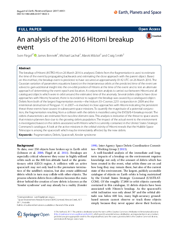
larger. The plot was created using ESA’s MASTER-2009 software (v7.2).
The spatial object density peak just below 800 km is created by the
fragments from the two debris clouds of the Iridium 33 and Cosmos
2251 spacecraft which collided in early 2009. The peak just above that
altitude is the debris from the Chinese anti-satellite test in which the
meteorology satellite Fengyun 1C was deliberately destroyed by a
ground-to-space missile (Liou and Johnson 2009; Johnson et al. 2007)
Contribution to Kessler syndrome
With respect to the Kessler syndrome, the orbit inclination and altitude at which the fragments orbit Earth
plays an important role. The overall collision risk is tied
to the spatial object density, to the relative velocities and
the remaining on-orbit time. Today, the regions in which
the risk for a catastrophic collision is highest are the
polar regions around 800 km altitude. In contrast to the
GEO region where the general orbiting direction of all
objects is the same (in the direction of Earth’s rotation),
the planes of the low Earth orbit (LEO) environment
polar orbits are evenly spread out around the Earth. This
causes the most likely impact direction on these orbits
to be head-on with a relative velocity of 14–15 km/s.
Large, massive spacecraft and rocket bodies which can
no longer be controlled within this region are deemed as
the most critical contributors: the probability for a collision is high and a conjunction will most likely lead to
the creation of hundreds or even thousands of new debris
which in turn may collide with other objects. Simulations
such as those presented by Kebschull and Radtke (2014)
have revealed that a number of Zenit-2 upper stages,
ESA’s Envisat, METOP-A and -B and also some Iridium
spacecraft are among the objects with the highest ‘environmental criticality’ rating.
The distribution in spatial object density for the orbit
altitude of interest is shown in Fig. 7. The orbit altitude of
significant other spacecraft is indicated.
Hitomi has an orbit altitude of roughly 570 km. It is
therefore not located in the critical region. Atmospheric
drag will cause the fragments to decay through other
regions which are less densely populated than at 800 km.
This also means that the debris will never travel through
the critical altitude band, and their contribution to the
Kessler syndrome is low.
Intact objects with potential close conjunction with Hitomi
debris
As can be seen in the Gabbard diagram (Fig. 4), the highest altitude of any fragment is about 580 km and atmospheric drag will continue to reduce their altitude over
time. Only spacecraft which are orbiting at this altitude or lower could potentially collide with one of these
fragments.
Transient objects A scan of the USSTRATCOM’s SSR
for 20 July 2016 reveals that about 600 intact objects
are in Earth orbit with apogee above and perigee below
580 km altitude. For 10 May 2016, the Satellite Database
of the Union of Concerned Scientists (UCS) (2016) contained 73 active spacecraft with these orbit characteristics. As long as objects spend most of their time above
580 km, the statistical risk of colliding with one of the
Hitomi fragments will be very low. They are therefore,
at least statistically speaking, the ones which have the
lowest nonzero probability for colliding with one of the
Hitomi debris.
Objects below 520 km The SSR contains a total of about
340 intact objects with orbits entirely below 520 km. The
UCS list about 120 active spacecraft for this region. As
�Flegel et al. Earth, Planets and Space (2017) 69:51
these orbits are below the current altitude of the Hitomi
fragments, a close conjunction may only occur in the
future when the drag-induced decay causes the debris
to pass through the orbital altitude regime of the listed
intact objects. The most important spacecraft in this category is the International Space Station which currently
is on a circular orbit just above 400 km.
Objects in ‘close orbital proximity’ Confining the orbits
to altitudes between 520 and 580 km results in a list of
objects which are at the same altitude as the Hitomi
debris is now. Their risk for a collision is immediately
affected by the new debris. In this region, the SSR contains 59 intact objects with orbit information; 12 of these
being upper stages and 47 being payloads. Of the rocket
bodies, five (all are SL-3 R/B) were launched before
1990. For the same altitude band, UCS published 31
active spacecraft. A subset of the data for these is given
in Table 5. In all, seven spacecraft are listed with launch
masses in excess of one tonne. From the standpoint of
the Kessler syndrome, these are the most critical objects
among the active spacecraft, as a catastrophic collision
involving one of these would create a large number of
fragments. The most notable entry in this list, however,
is the Hubble Space Telescope (HST) which has an orbit
altitude of 560 km. The collision velocity in the event
of a conjunction would be lower than the 14–15 km/s
observed in polar orbits as the HST and Hitomi have very
similar orbit inclinations (28° and 31°, respectively). The
exact value depends largely on the relative separation of
the right ascension of ascending node. For similar values, the orbital planes will be roughly aligned and relative
velocities will be very low. If they have a relative separation close to 180°, a conjunction near the line of nodes
could occur in which one object is travelling on a shallow
south–north trajectory while the other is moving in the
opposite direction. This configuration would result in a
collision velocity similar to the orbital velocity (≅7 km/s).
Conclusion
The event time was estimated to March 26, 01:42 ± 00:14
by calculating the minimum distance between the propagated states of the debris and of Hitomi. The location of
the object at the estimated time of the event was compared to solutions for event locations obtained from
solving of the Gaussian variation of parameters equations. Based on these results, the argument of latitude at
the time of the event is estimated to have been u ≅ 83◦.
Solving of the equations revealed that radial, along-track
and cross-track velocity changes in the order of 7.9, 0.3
and −1.4 m/s were imparted on the main body due to
the fragmentation. By combining the normal probability
density functions from the minimum distance approach
and from the event location solutions, an event epoch
Page 11 of 13
which takes into account solutions in different parameter
domains was obtained which places the event 10–11 min
later which is well within the original estimate. This solution’s accuracy in the time domain depends on the realism of the true anomaly evolution in the vicinity of the
event epoch. The accuracy of this solution can therefore
only be obtained if the accuracy of the orbit data upon
which it relies is available. As this is unfortunately not
the case, the absolute accuracy of this solution cannot be
stated.
Due to the orbit altitude of the event, the debris from
the Hitomi anomaly does not fuel the critical polar orbit
region at altitudes around 800 km. Of the eight fragments which remain in orbit, it was estimated that all but
Hitomi’s main body should deorbit before or during the
upcoming solar maximum around 2025. The main body
will likely remain in orbit for a few decades. Statistically,
the probability that this object may be involved in a collision is much higher than for the fast decaying fragments.
The conjunction analysis revealed that a number of
debris from the breakups of the Iridium 33, the Cosmos
2251 and the Fengyun 1C spacecraft were in Hitomi’s
orbital vicinity with potential for close conjunction.
This observation highlights the impact of high-energy
fragmentations on the operational safety of spacecraft
in Earth orbit. Had one of these objects struck Hitomi’s
body, the expected number of debris would in most cases
have exceeded the number of currently tracked objects
for Hitomi. The catastrophic collisions between Hitomi
and the Delta 1 debris or the Dnepr 1 rocket body especially would have been very damaging to the environment with thousands of debris larger than 10 cm being
created. The simulations using the EVOLVE-4 model also
showed that a non-catastrophic collision with a debris
with a mass of about 45 g could potentially produce a
similar number of large debris as have been catalogued.
For spherical sodium–potassium debris released from
a Russian Buk reactor, this would relate to a diameter
of about 4.6 cm. A steel or aluminium debris of similar
mass would have similar or smaller sizes. As this size is
below the USSTRATCOM’s current catalogue threshold
of about 10 cm, the modelling results do not exclude a
non-catastrophic collision with such an object. Just the
same, JAXA’s assessment that the breakup was a result
of a combination of operational and design flaws is just
as plausible. The current analysis does not allow any conclusion concerning the mechanism which caused the
breakup.
A total of 59 intact objects are included in the
USSTRATCOM’s catalogue whose collision risk is immediately affected by the Hitomi debris. Of these 59 objects,
12 are rocket bodies, and 47 are active and inactive
spacecraft. The most prominent active spacecraft which
�Flegel et al. Earth, Planets and Space (2017) 69:51
Page 12 of 13
Table 5 List of active spacecraft within 520–580 km orbital altitude (UCS 2016)
Int.-desig.
Name
Country
Perigee (km)
Apogee (km)
Incl. (°)
2015-049N
XW-2B (CAS-3B)
China
520
539
97.46
2015-049J
XW-2D (CAS-3D)
China
520
539
97.46
2015-049R
KJSY-1 (Kongjian Shiyan-1)
China
520
540
97.46
2015-049V
XC-1 (Xingchen 1)
China
520
540
97.46
2015-049S
XC-2 (Xingchen 2)
China
520
540
97.46
2015-049T
XC-3 (Xingchen 3)
China
520
540
97.46
2015-049U
XC-4 (Xingchen 4)
China
520
540
97.46
2015-049M
XW-2F (CAS-3F)
China
520
540
97.46
2015-049W
Zijing 1
China
520
540
97.46
2015-049K
LilacSat-2
China
520
541
97.47
2015-014A
Kompsat-3A
Sth Korea
522
540
97.5
2006-029A
Genesis-1
USA
522
569
64.5
2015-077E
Galassia
Singapore
529
549
14.98
2015-077C
Athenoxat-1
Singapore
532
550
14.98
2015-077A
Velox C1
Singapore
533
550
14.98
2015-077B
Kent Ridge 1
Singapore
534
551
14.98
2015-077D
TeLEOS 1
Singapore
535
550
15
2002-004A
HESSI (RHESSI)
USA
535
551
38
2013-042A
Kompsat-5
Sth Korea
535
552
97.6
2015-077F
Velox 2
Singapore
537
550
14.98
2008-029A
GLAST
USA
537
556
25.6
2007-006E
Falconsat-3
USA
538
540
35.4
2012-017A
RISat-1
India
538
541
97.6
2007-006F
CFESat
USA
538
544
35.4
2007-015A
AIM
USA
544
552
97.9
2005-025A
Suzaku (Astro E2)
Japan/USA
548
558
31.4
2013-015E
BeeSat-3
Germany
554
581
64.8
1990-037B
Hubble Space Telescope
ESA/USA
555
559
28.5
2013-015G
BeeSat-2
Germany
555
579
64.8
2006-021A
Resurs-DK1
Russia
564
571
69.9
2001-007A
Odin
Sweden
569
573
97.6
is affected by the debris is the Hubble Space Telescope
whose orbit is just 10 km below that of Hitomi. Other
active spacecraft with significant mass which are affected
include the inflatable Genesis-1 habitat, Kompsat-5,
GLAST, RISat-1, Suzaku and Resurs-DK1. The draginduced gradual decrease in orbit altitude of the Hitomi
fragments will cause these objects to pass through the
orbit regime of other, low-orbiting spacecraft, whereby
new close conjunctions may occur. One of these objects
is the International Space Station.
Abbreviations
ACS: attitude control system; BCEM: ballistic coefficient estimation method;
DRAMA: Debris Risk Assessment and Mitigation Analysis; EOB: extensible
optical bench; EOS: Electro-Optic Systems; ESA: European Space Agency;
HST: Hubble Space Telescope; intact: active and passive spacecraft and rocket
bodies; JSpOC: Joint Space Operations Center; JST: Japan Standard Time;
LEO: low Earth orbit; OSCAR: Orbital Spacecraft Active Removal; PDF: probability density function; RCS: radar cross section; RW: reaction wheel; SERC:
Launch mass > 1 t
*
*
*
*
*
*
*
Space Environment Research Centre; SGP4: Simplified General Perturbations
4; SOCRATES: Satellite Orbital Conjunction Reports Assessing Threatening
Encounters in Space; SSR: Satellite Situation Report; TLE: two-line element;
USSTRATCOM: United States Strategic Command; UTC: Universal Time Coordinated; VoP: variation of parameters.
Parameters
a: semi-major axis; e: eccentricity; i: inclination; Ω: right ascension of ascending
node; ω: argument of perigee; ν: true anomaly; u: orbit angle; v: velocity; ∆v:
velocity change.
Authors’ contributions
SF performed the event location analysis and the impact on the environment
analysis. He aided in the design of the study and performed final editing
and submission of the manuscript. JB carried out the event time estimated
and conjunction analysis and drafted the first version of the manuscript. ML
analysed the radar cross section of the debris, inferred object sizes used in
the conjunction analysis and was instrumental in the conjunction analysis
results evaluation. MM is in charge of developing the GPU-based conjunction
assessment software and developed software which was key for the event
location analysis. CS initiated the study, participated in the design of the study
and helped to draft the manuscript. All authors read and approved the final
manuscript.
�Flegel et al. Earth, Planets and Space (2017) 69:51
Author details
1
Space Environment Research Centre (SERC) Limited, Weston Creek, ACT
2611, Australia. 2 Electro Optical Systems (EOS), Weston Creek, ACT 2611,
Australia.
Acknowledgements
The authors would like to acknowledge the support of the Cooperative
Research Centre for Space Environment Management (SERC Limited) through
the Australian Government’s Cooperative Research Centre Programme.
Furthermore, the authors wish to thank the reviewers of the manuscript
for their insightful and helpful comments.
Competing interests
The authors declare that they have no competing interests.
About SERC
To help address the issues involved with safe spacecraft operations in the
presence of space debris, the CRC for Space Environment Management, managed by the Space Environment Research Centre (SERC), has been established
(www.serc.org.au). Key developments are being made in the positioning
accuracy especially for GEO and HEO objects through the application of
adaptive optics astrometry wherein atmospheric distortions are removed
through adaptive optics. Attitude estimation from light curve analyses will
allow incorporating non-spherical object geometries into orbit determination
and prediction which will also aid in decreasing the uncertainty in conjunction assessments. By developing operational software which is designed to
run on a single CPU, parallelised on multi-core CPUs or massively parallelised
on GPUs while retaining double precision accuracy, high-accuracy approaches
which would ordinarily not be feasible due to long processing times can be
employed routinely. It was shown in previous research that orbital propagation can benefit greatly from massively parallel hardware architectures such as
graphics processors (Möckel 2015). A core effort within SERC is to implement a
high-accuracy all-on-all conjunction assessment for large object catalogues in
this framework which is expected to reduce the required processing time considerably. SERC is presently in the process of setting up its first self-sustained
catalogue of LEO to GEO objects which will be maintained using multiple passive and active optical instruments and in-house developed scheduling software for optimal sensor tasking. One of the outputs SERC is working towards
is the ability to provide high accuracy conjunction assessments so as to help
reduce the number of collision avoidance manoeuvres. Furthermore, an active
ground-based laser collision avoidance system using photon pressure is being
developed which will support debris mitigation measures.
Publisher’s Note
Springer Nature remains neutral with regard to jurisdictional claims in published maps and institutional affiliations.
Received: 7 September 2016 Accepted: 4 April 2017
References
Flegel S, Gelhaus J, Möckel M, Wiedemann C, Kempf D, Krag H, Vörsmann P
(2011) Maintenance of the ESA MASTER model–final report. Technical
Report ESA Contract Number: 21705/08/D/HK, European Space Agency
Hoots FR, Roehrich RL (1980) Spacetrack report no. 3—models for propagation of NORAD elements sets. Spacetrack Report, vol 3(3)
Inter-Agency Space Debris Coordination Committee—Working Group 2
(2013) Stability of the future LEO environment. Technical Report Action
Item 27.1, Inter-Agency Space Debris Coordination Committee
JAXA (2016) Hitomi experience report: investigation of anomalies affecting the
x-ray astronomy satellite “Hitomi” (ASTRO-H). Press release, JAXA, 31 May
2016. http://global.jaxa.jp/projects/sat/astro_h/files/topics_20160531.pdf
Page 13 of 13
Johnson NL, Krisko PH, Liou JC, Anz-Meador PD (2001) NASA’s new breakup
model of EVOLVE 4.0. Adv Space Res 28(9):1377–1384. doi:10.1016/
s0273-1177(01)00423-9
Johnson NL, Stansbery E, Liou J-C, Horstman M, Stokely C, Whitlock D (2007)
The characteristics and consequences of the break-up of the Fengyun-1C
spacecraft. In: Proceedings of the 58th international astronautical congress. International Astronautical Federation, Sept 2007. Paper Number
IAC-07-A6.3.01
Johnson NL, Stansbery E, Whitlock DO, Abercromby KJ, Debra S (2008) History
of on-orbit satellite fragmentations, 14th edn. Technical Report NASA/
TM-2008-214779, Orbital Debris Program Office, National Aeronautics
and Space Administration
Kebschull C, Radtke J (2014) Deriving a priority list based on the environmental criticality. In: International astronautical congress, Sept 2014.
IAC-14,A6,P,48x26173
Kelso TS, Alfano S (2006) Satellite orbital conjunction reports assessing threatening encounters in space (SOCRATES). In: Proceedings of SPIE, 6221,
modeling, simulation, and verification of space-based systems, vol III, p
622101. doi:10.1117/12.665612
Kelso TS (2009) Analysis of the Iridium 33-Cosmos 2251 collision. Adv Astron
Sci 135(suppl 2):1099–1112
Kessler DJ (1991) The limits of population growth in low Earth orbit. Adv Space
Res 11(12):63–66
Krisko P (2011) Proper implementation of the 1998 NASA breakup model.
Orbital Debris Q News 15(4):4–5
Liou J-C, Johnson NL (2009) Characterization of the cataloged Fengyun-1C
fragments and their long-term effect on the LEO environment. Adv
Space Res 43:1407–1415. doi:10.1016/j.asr.2009.01.011
Möckel M (2015) High performance propagation of large object populations
in earth orbits. Ph.D. thesis, Technische Universität Carolo-Wilhelmina zu
Braunschweig. doi:10.5281/zenodo.48180
Sang J, Bennett JC, Smith CH (2013) Estimation of ballistic coefficients of low
altitude debris objects from historical two line elements. Adv Space Res
52(1):117–124. doi:10.1016/j.asr.2013.03.010
UCS (2016) Union of Concerned Scientists Satellite Database. Retrieved May
2016. https://s3.amazonaws.com/ucs-documents/nuclear-weapons/satdatabase/2-25-16+update/UCS_Satellite_Database_1-1-16.xls
Vallado DA, McClain WD (2013) Fundamentals of astrodynamics and applications. Space Technology Library, 4 edn. ISSN:9781881883203
Wiedemann C, Flegel S, Gelhaus J, Krag H, Klinkrad H, Vörsmann P (2011) NaK
release model for MASTER-2009. Acta Astron 68:1325–1333
Wiedemann C, Flegel S, Kebschull C (2014) Additional orbital fragmentation
events. In: Proceedings of 65th international astronautical congress, 2014.
IAC-14.A6.P.57
�
 Michael Lachut