Using Downloaded Demonstration Software to Promote
Software Products in Global Markets: A decision-making
model for software vendors
Tevfik Dalgic
∗
and Metin Çakanyıldırım
School of Management, University of Texas at Dallas, Richardson, Texas 75083.
May 3, 2003
Abstract
This paper attempts at developing a model for the software vendors to market their software products globally
by using the Internet. Allowing the buyers to download and test demonstration versions of software programs
for a certain time period is an industry practice for many software vendors. Due to the standard nature of the
software products and availability of them for anybody who has necessary technical facilities and knowledge
of the Internet usage, this model could be a successful decision-making tool for global marketing activities of
software vendors.
∗
For correspondence: tdalgic@utdallas.edu
�1
Introduction to Internet and International Marketing
The Internet is the primary driving technology behind electronic commerce, and gives marketers unprecedented
capabilities. Most problems inherent in the marketing of many types of goods and services internationally do
not matter on the Internet. The Internet not only overcomes limitations of international goods and services
marketing, but also creates undreamed of foreign market opportunities for many firms. The low entry barrierscosts of setting up and maintaining an information Web site or electronic storefront-have made the global
marketplace an easier playing ground for businesses which can bypass physical networks of intermediaries and
bring goods and services directly to customers anywhere. The Internet has also helped improve the internal
efficiencies of supply chains by electronically connecting the participants according to [6].
The Internet medium affords marketers the ability to make available full-color virtual catalogs, provide
on-screen order forms, offer online customer support, announce and even distribute certain services easily, and
elicit customer feedback. ”Any firm that uses the Web has an international presence” [40] .The growing volume
of e-Commerce has opened up new areas of communication, cooperation, and coordination among consumers,
business units, and trading partners around the World. The Internet has become not only the main medium
for marketing, but also the main communications medium for international business. It simply promises to
revolutionize the dynamics of international business [?]. The Internet reduces the importance of geographic
distance tso insignificant levels, at the same time it opens up significant opportunities for reaching international
customers. [26], point out that marketers are adding on-line channels to find, reach, communicate, and sell”
and that companies small and large are taking advantages of cyberspace’s vanishing national boundaries.
The Internet is perceived as ”captivating people on every continent in virtually every culture, and in many
languages.[?]. [15] observed that internationalization is one striking feature of the Internet.
[?] predicted that the Internet will accelerate the internationalization of small and medium-size enterprises.
[27] observation brings a new dimension. He concludes; the Internet is expected to offer smaller firms ”a
level playing field” in relation to their larger competitors by reducing the traditional importance of scale
economies, making global advertising more affordable, and extending smaller firms’ market reach globally.
Similar observations have been made by [?] and others [21].
Among many, [33] described the Internet as ”the most important innovation since the development of
the printing press” which may ”radically transform not just the way individuals go about conducting their
business with each other, but also the very essence of what it means to be a human being in society.” In
the last five years, the number of Internet users has increased more than nineteen fold – over 100 million
[?]. Several studies are conducted at several levels in several organizations to develop models to explain the
dissemination of the Internet usage among countries. For example, Paris-based think-thank the Organization
for Economic Cooperation and Development (OECD) [34] has applied a Life-Cycle approach to develop stages
of development of E-Commerce. Ongoing analytical work at OECD uses a life-cycle model to highlight the
phases of e-Commerce. Each phase can be measured with different sets of indicators that also correspond to
different policy concerns for governments. OECD experts state that we are still in the readiness phase of the
cycle. Figure 1 explains this relationship.
Both in business-to-business and business-to-consumer marketing domains, the Internet affects activities
that occur through three types of marketing channels: communication channels, whose primary functions are
to inform buyers and prospective buyers about availability and attributes of a seller’s products/services and
to enable buyers and prospective buyers to communicate with sellers; transaction channels, whose primary
function is to facilitate economic exchanges between buyers and sellers; and distribution channels, whose
1
�Level of ECommerce
Activity
Intensity
Size
Readiness
Efficiency gains
Employment, skill
composition,
work organization
Current and
potential usage
Time
Figure 1: Life-cycle of e-commerce activity [34].
primary function is to facilitate physical exchanges [38]. However, there are times that the appropriateness of
the Internet for international marketing is presumed without a critical examination of the foundations upon
which international marketing rests [44]. Many assume that e-Commerce in emerging markets will evolve along
the same lines as it has in the US, North America, and in Western Europe, and that is simply not true [?].
In reality, the growth of e-Commerce is based on a complex network of various elements such as information
technology, where developed and developing countries are in different development stages [?]. [18] state that a
Net connection can ”substantially improve communications with existing foreign customers, suppliers, agents
and distributors, identify new customers and distributors, and generate a wealth of information on market
trends and on the latest technology and research and technical developments”.[28]asserts that the Internet
enables small firms to grow without expanding physically or incurring relocation expenses, and allows them to
advertise and promote themselves globally at minimal cost. Customers, care little about the physical size or
remoteness of a supplier, provided high quality products at fair prices are delivered.[28].
Despite very optimistic future scenarios, present applications and probable difficulties and low level development of the Internet infrastructure in different parts of the world; The Internet has remains as an important
tool of marketing, communications and product development in many areas of business; both at national and
international levels.
2
�2
Software marketing on the Internet
However the use of the Internet as a channel for physical product delivery is limited. With the exception
of products that can be ”delivered” electronically, such as music, software, newspapers, magazines, travel
tickets, and financial investments, most products must still be delivered via traditional logistical means [43].
Software is an electronically delivered product and do not need to be distributed by the traditional distribution
channels. This creates an opportunity for global software producers to distribute their products, because the
Web marketer has a global reach with the elimination of obstacles created by geography, time zones, and
location [?]. Especially software companies put up their products on the Internet. They also explain potential
benefits of their products and usage. Potential buyers can even discuss the capabilities of the software before
the purchase. This has created opportunities for global software producers to distribute their products, because
the Web marketer has a global reach with the elimination of obstacles created by geography, time zones, and
location [23]. According to [1], many companies, including GE, Bank of America, Target and American Express,
are going offshore to develop and maintain their software. A recent survey by the Indian National Association of
Software and Service Companies found that almost two out of five Fortune 500 companies currently outsource
some of their software requirements to India. In 2000, North American companies alone spent $114 billion on
in-house software development, contracting, and purchases-and costs will only go higher as additional basic
business processes are conducted over the Internet [1]. Therefore, the Internet has become an effective medium
for marketing for both local and international customers. This is more so for small companies that cannot afford
to promote their products through more expensive marketing channels, promotional and publicity campaigns
and industrial fairs. The Internet has decreased marketing expenses for many medium and small companies to
go international beyond their home country markets [10] [14]. Despite the vast opportunities provided by the
Internet to the marketers, there are some issues to be addressed, like cultural and local environmental factors.
As observed in [23]: ”Cultural barriers remain To avoid cultural pitfalls, many small entrepreneurs without
broad contacts use Internet discussion groups to become familiar with local customs, trends, and laws.”
The low entry barriers (costs of setting up and maintaining an information Web site or electronic storefront)
have made the global marketplace an easier playing field for businesses which can bypass physical networks of
intermediaries, and bring goods and services directly to customers anywhere. Any firm that uses the Web has
an international presence [23]. Due to the standard nature of the software products, marketing them globally
to those customers with similar needs and desires seems to be very appropriate method of distribution and
many software vendors have been using this method. In emerging markets, the opportunities for conducting
electronic transactions over the Internet are limited mainly for two reasons:
Credit cards are not as extensively used in developing countries as they are in developed countries; and
people are often reluctant to conduct financial transactions over the Internet due to the unavailability of
secure connections [41];[11]. The first problem is mainly economic and cultural, whereas the second problem
is infrastructural. Internet marketers will do well to primarily target business customers in emerging markets,
but they should not ignore consumers altogether.
[15] observed that Internet access transcends national boundaries, as anyone anywhere can communicate
with others and shop anywhere. The asserted internationalized nature of the Internet has encouraged companies
to embrace it as a way of accessing bigger markets that were not previously open to them. As [51] suggests,
”once you are on the web, you are immediately a global company”. Research activity on Internet shopping or
usage has increased steadily in recent years. [21]; [33]; [47].
The view of the global values of the Internet should result in Internet retailing appealing to similar consumer
segments irrespective of country. Many emerging markets have segments-the size of which is more attractive in
bigger markets such as India, Indonesia, Brazil, Poland, Turkey or Mexico- of affluent urban upwardly-mobile
3
�professionals having an online presence. Effective application of information technology (IT) is considered a
requirement for organizations that wish to compete in the global marketplace of the future.[4]. The Internet can
become a new medium for advertising and public relations, a new way for enhancing customer service, a new
channel for distributing products, and a new opportunity for the improvement of marketing effectiveness.[38].
[1] argued that computer chips, automotive electronics, color films, pharmaceutical, chemicals, telecommunications, and network equipment are fast changing in nature but are standardized, thereby allowing them to be
more readily internationalized. They point out that music attracts consumer segments that transcend political
and geographical boundaries.
When a software vendor puts its products on the Internet to be downloaded for trial or demonstration and
testing by the potential buyers, it is also deciding on the duration of this trial period in terms of how many
days this product could be used and tested by them. The decision about the trial period is very important for
the vendor which may play a role of providing a maximum return. This paper will try to develop a model for
an optimum trial period for the software vendors.
Section Towards an optimal model for trial period
In this paper we will study how customers use the demonstration mechanism (“demo” from now on) to
evaluate products, such as information products (software, electronic magazines, archives) and cars. During
demo, customers are given free access to products (or some versions of them) to experiment with product
features and to acquire product specific knowledge. The knowledge acquired with experimentation accumulates
over time and is never forgotten. We can envision the knowledge about a product starting from a certain level
and increasing to another level in time as suggested in [37]. We will use this learning process to analyze the
evaluation of the products. Evaluation will correspond to mapping the product specific knowledge at the end of
the demo to product value. We will present customers’ buy-or-not decision in conjunction with product value
and price. In this context, demo is a valuable mechanism to convince customers of the high value of products
as confirmed in [14] by an AOL manager who reports that: “the trial offers are worthwhile because nearly
three-quarters stay on as full-paying members.” We will introduce two principal demo strategies and study the
trade offs involved in finding optimal strategy parameters.
In practice, the popularity of demo is rising because of three fundamental factors. First, products are
becoming complex, this trend is especially pronounced in the software industry. This makes it harder for
vendors to communicate the features of the products to potential customers. Traditional promotion channels,
such as advertisements and brochures, are not very effective for complex products. Realizing this, vendors are
allowing customers to have first hand experience of products during demo. Second, technology has developed
enough to make demo a viable option for promotion. Doubtlessly the biggest contributor in this respect is the
Internet. It provides easy access to product information and sometimes to the product itself. For example,
demo versions of informaton products are distributed over the Internet. Using cookies, it is technologically
possible to disable a product at the end of demo and prohibit multiple demo accesses/downloads of the same
product onto the same computer. Finally, two conditions must be satisfied roughly before a purchase: first
product awareness and then sufficiently high perceived (by customers) product value. The technology is making
the product search so easy that focus has been shifting from increasing product awareness to convincing the
customer for a purchase.
We will not model production costs explicitly and assume that every extra unit of sale brings in a constant
amount of profit. This is especially valid for informaton products because once the first product is designed
and developed, the others can be produced at a negligible cost. It is supported by the observation that
customer feedbacks are not implemented immediately but are considered for the future releases of software,
so additional customers / feedbacks do not increase the production cost of the current release. This allows us
to use “profits” and “revenues” synonymously. We assume that evaluation process is the same for individuals
4
�making purchase decisions for themselves or for an organization, so observations of this paper apply to both
individuals and organizations who would be called customers. We assume that product testing causes negligible
costs to customers.
The Internet allows small and large international companies market products to a large customer base
scattered around the globe by eliminating obstacles created by geography, time zones, and location [40]. This is
more so for small companies which cannot afford to promote their products through more expensive marketing
channels, promotion and publicity campaigns and industrial fairs. The Internet has decreased marketing
expenses for many medium and small companies to go international beyond their home country markets [20].
Especially information products are put up on the Internet to illustrate ther capabilities to potential customers
before the purchase: This has created opportunities for global software producers to distribute their products
[2], many companies, including GE, Bank of America, Target and American Express, are going offshore to have
their software developed and maintained. Because of not having an established brand name, small and global
software producers have hard time in selling their products. On the other hand, customers find it equally hard
to find and evaluate information products to satisfy their needs. This hardship is more pronounced for small
companies which cannot afford to dedicate large resources to product evaluation [22]. Demo strategies solve
not only vendors’ promotion problem but also help customers to evaluate products.
Product evaluation relates to new information gathering, updating existing information and perception
formation tendencies of customers as they use or test products. [29] suggests that beliefs about an attribute
of a product is a weighted combination of initial beliefs and observed beliefs. [8] argues that, while choosing a
auto repair service center, a consumer’s experience with a center is more important than externally obtained
information on that center. [5] studies how customers’ experience with a product determine their satisfaction.
[12] study consumers’ brand choice process while product diffusion is happening. [7] argue that customers
may construct preferences over time rather than having a stationary set of preferences. This can happen when
there are contingencies among preferences where the value of each preference depends on the value of other
preferences. On the other hand, [32] investigated the issue of persistent preferences for product attributes
which are always favored over other preferences. It also considers product trial as a necessary tool to develop
an opinion about a brand as a result of key attributes of that brand.
Some product attributes (price, user friendliness) can be more easily evaluated than others (reliability,
compatibility). Those attributes that take time to be evaluated cause product information to be incomplete
initially, say at the first contact with the product. In a recent review, [25] mentions two approaches about
treating incomplete information. Incomplete information generally causes customers to discount the value of
a product and/or ignore the attributes with incomplete information. [42] show that when consumers have
uncertain beliefs about products, they offset the expected utility of products by a certain multiplier of the
variance of beliefs about the utility. Beliefs about an attribute can also be obtained by updating prior beliefs
with observed beliefs in a Bayesian fashion [42].
Marketing literature have investigated product evaluation from different points of view. [19] categorizes
products according to how attributes are learned: play products, functional products, time products, undemonstrable products. It places information products into time product category, saying that discovery of
their attributes take substantial time. [24] and [52] distinguish attributes as experimental (called search in
[52]) attributes which are observed after some use, and nonexperimental (called learning in [52]) attributes.
According to [19], attributes of learning (search) products can be evaluated before (only after) the purchase.
[24] argues that product trials have powerful influences on brand evaluation and considers only experimental
attributes during trial.
Information products are not physical goods so they do not wear down. Once they satisfy customer
needs, they may be used for a long time unless the needs change. Although each manufacturer has its own
5
�development plans, upgrades take place frequently. Consequently, customers often buy different versions of a
product. Since different versions have different functionality, we treat every version as a different product. As
a result, all customers are first-time buyers. Demo strategies are logical approaches to attract first time buyers.
Unfortunately, most of the previous studies address buy-or-not decisions for repeat buyers. In the context
of first time buyers who evaluate a product and decide during the product demo, literature lacks a study of
product valuation, pricing and associated profit. Therein lies the contribution of this paper where an attempt
is made for using demo as a promotion method and its interaction with pricing.
The rest of this paper is organized as follows: In the next section, we introduce version and phase strategies,
and obtain product values as a sum of values of evaluated features. In Section 3, we express vendor profits and
study their unimodality in decision variables. This is ensued by numerical examples and associated managerial
insights. Finally, we provide a brief conclusion in Section 5. To maintain the flow of our arguments, we postpone
most of the proofs to the Appendix.
3
A Model of Product Evaluation
Customers want products that can reliably perform certain functions and meet the current needs. When vendors
release products, they claim that products perform some functions. However, customers cannot be certain
about the performance of a new product because of potential problems such as low reliability, bugs, lacking
compatibility with existing products. Thus, customers prefer to evaluate product performance preferably at
their own site, before paying for them.
We envision a product as a bunch of features, where we use the term “feature” to mean a single function
of given product. During a demo, customers evaluate the features one by one to see if they are functioning
properly. At any time during the demo, customers have a set of features already evaluated and the remaining
set of features to be evaluated. The value of the evaluated and properly functioning features can be assessed
right away. However, the value of features to be evaluated is uncertain because customers have incomplete
information about them. Product evaluation can be done in several ways. In the first approach, customers
learn the features of a product one by one while evaluating it. Customers may tolerate a couple of bugs or
unexpected outcomes during learning, although these problems may lower the perceived value of the product.
Too many problems will naturally make customers reject the product. In the second approach, customers test
the features of the product with test cases prepared in advance [31]. Naturally, the outcome of these tests
must be verifiable independently, without using the product being tested. Some vendors use test cases to test
products before the release. [35] and the references therein provide some literature on economics of product
testing by vendors.
Two demo strategies are currently popular among vendors: demo phase and demo version. In the demo
phase strategy, customers have access to the entire product for a limited time, i.e. during demo phase. In
the demo version strategy, customers are given a limited (demo) version of the product for forever. The demo
version includes only a subset of the features of the full version. Since learning a product requires more time
than testing it, customers who evaluate a product by testing are less time sensitive. Since the demo version
strategy does not account for time, it models testing better than learning. Both demo phase and version
strategies can be relevant for learners, although the demo phase explicitly studies learning speed of customers
and hence provides a richer model.
At the beginning of a demo, customers may know all features (promised to work properly) if vendors
mention these in product manuals. In practice, the total number of features is much larger than the number
of features learned during a demo. Software tend to have many features, some of which are never used even
6
�years after the purchase. Along these lines, [36] says that:“. . . our experience tells us that the typical UNIX
users only use about 40% of the tools and utilities available to them.” Let U be the set of features of a product
and set U = |U|, these observations motivate taking U as infinity to obtain limit results in what follows. Let S
be the set of features that function properly according to customers’ specifications/needs. We call features in
S as successful (good) features and the others as defective (bad) features. Since S usually relates to customer
specifications, a vendor cannot determine S. Even when S is independent of customer specifications, the vendor
may not know the set of the good features [35]. Neither demo phase nor demo version strategy allows customers
to discover entire S because customers do not have enough time or all features, respectively, in these strategies.
Consequently, demo allows customers only to estimate S.
We define the value of product features using a value function V . We require
P two natural axioms on V :
Positivity: V (∅) = 0 and V (C1 ) ≤ V (C2 ) if C1 ⊆ C2 ⊆ U. Additivity: V (C) = k∈C V ({k}) for all C ⊆ U.
Positivity merely states that the value of extra features cannot be negative. Additivity can be motivated
by assuming that there is neither synergy nor duplicity among product features. The driving force behind
additivity is independence of features values. For example tution fees are proportional to credit-hours taken
at certain unversities. Another example, McGraw Hill sells books chapter by chapter and prices each chapter
separately. These are because the value of a course (chapter) is considered as independent of other courses
(chapters). Accounting for product values without additivity can be hard to manage, so additivity is often
built-in to pricing models.
We use value function to assign a monetary value to product features. The product value is V (U ∩S) = V (S)
but S will appear as a random set to a customer and ranges from ∅ to U. Let p be the success probability for
each feature in U . We assume that this probability is the same for all features. Then, treating value functions
as random variables we obtain that
¾
½
Yi with probability p i.e. feature i is good
V ({i} ∩ S) = Ȳi =
0
with probability 1 − p i.e. feature i is bad
where Ȳi (Yi ) is the value of ith feature (given that it is good).
Customers evaluate features in a sequence, possibly going from a simple feature towards a more complicated
one. There can be precedence relations among features forcing the customer to evaluate one feature before
another. In the ultimate case, these relations will imply a complete order. We depicted three cases of product
features in Figure 2. The evaluation sequence of features is irrelevant for our analysis of version strategy. For
the phase strategy, we assume there is a sequence determined a priori to our analysis, and number the features
according to this sequence.
Customers evaluate features one by one to build Ct , the set of features already evaluated by time t, so
C0 = ∅. Since we assume that the acquired knowledge is not forgotten, Ct never contracts, i.e. Cs ⊆ Ct for
s ≤ t. Ct ∩ S is the set of good features that are evaluated by t. At time t, the (observed) value Vt of a product
is:
V (t) = V (S ∩ Ct ) and V0 = 0.
(1)
At time t, Ct is observed so Ct ∩ S is not a random set anymore, but U − Ct is not observed and ((U − Ct ) ∩ S)
is a random set. V (S) can be significantly or slightly larger than V (t) depending on the success rate of the
features in U − Ct . Using (1) and the Positivity axiom,
t→∞
V (s) = V (S ∩ Cs ) ≤ V (S ∩ Ct ) = V (t) for s ≤ t and V (t) −→ V (S)
7
(2)
�2
5
4
1
U
6
3
Unordered features
2
5
4
1
U
6
3
Features in a full (chain) order
2
5
4
1
U
3
6
Features in a partial (precedence) order
Figure 2: Unordered, fully ordered and partially ordered product features.
The process V (t) is nondecreasing in a sample path sense. For the case of version strategy with N features, the
product value can be obtained by setting t ← ∞ and S ← S ∩ {1, . . . , N }. From a customer’s point of view,
the perceived value of the product is nondecreasing in time or the extent of the demo version so this explains
the vendor’s motivation to extend the demo length and expand the demo version.
3.1
Demonstration version strategy
In the demo version strategy, vendors hand out a demo product with limited features to customers who base
buy-or-not decision of the full product on the evaluation of the demo product. For example, Amazon makes
several chapters of books available for promotion. Newspapers use this strategy by giving free access to their
web sites where only certain news articles are featured to promote the paper copy. It is possible to listen to the
first 30 sec. of songs on the Internet without buying them. In these examples there is not much to learn about
features, rather customers glance at demo versions to decide if they like it. Thus, the evaluation resembles
testing rather than learning.
Remember that N is the number of features available in a demo version. Unless evaluating features cost
substantially with respect to the price of the software, customers will evaluate all the available features before
committing to buy a product. Then the set of features evaluated just before buy-or-not decision is {1, . . . , N }.
The value of these features is VN
X
VN = {
Yi with probability XN (p) = |C| for all C ⊆ {1, . . . , N }}
(3)
i∈C
where XN (p) denotes a binomial random variable with N trials and p probability of success.
8
�In general, a vendor supplies many customers. Depending on potential usage, current needs, different
customers may attach slightly different values to the same feature. Although we may argue for deterministic
feature values for a single customer, those values become stochastic for a randomly chosen customer from a
population. From vendor’s point of view, feature values are then stochastic variables. If customers divide
product features into similar groups in terms of hierarchy/importance, features are likely to have similar values
(in a stochastic sense). For example, a customer can give edit and view features of Microsoft Word equal value
and treat these as features. It is also possible to go down one step below in command hierarchy and treat
all subcommands of edit and view as features with equal value. If feature values are not similar, features can
be divided into smaller pieces or united together to have more or less identical feature values. Motivated by
these observations, we use identically and independently distributed (iid) random variables to represent feature
values. This allows us to express the product value without studying subsets of {1, . . . , N } as in (3) and yields
VN =
N
X
XN (p)
Ȳi =
i=1
X
Yi
(4)
i=1
We scale the feature values by E(Yi ) so that new feature values have expected value of 1 and variance of σ 2 .
We can specialize VN for two practical cases
Case 1. Many features are tested : When many features are included in the demo version, i.e., N is large.
Case 2. Deterministic values: If vendors know the value customers attach to each feature with certainty, then
Yi = 1 for all i after scaling values by their expected value.
Let VN1 and VN2 denote the value of the product under Cases 1 and 2:
VN1 = N (N p, N (p σ 2 + p − p2 )) and VN2 = XN (p)
(5)
where N denotes a Normal random variable. Although VN1 converges to the Normal distribution, we write it
as equal for notational simplicity. VN1 is obtained by applying the central limit theorem to the random sum of
(4). Since knowing feature values reduces uncertainty, VN2 is less variable than VN1 . We will use the valuations
of (5) to compare version and phase strategies.
3.2
Demonstration phase strategy
Some vendors choose to promote their products by allowing customers to evaluate full versions of the products
during a demo phase. Demo phase lengths are 14 days for Encyclopedia Britannica, 30 days for EditPlus
editor, 6-12 months for the computer software that comes with college textbooks and 1000 hours for AOL
membership. These products are more complicated than those of demo version and they must be learned.
Actually this strategy seems to be more commonplace than the version strategy in practice.
Different customers tend to have have different learning times for the same feature, because of their (educational / professional) backgrounds and previous exposure to similar features. As we argued for stochastic
feature values before, we can argue for stochastic learning times. The traditional way of finding out learning
times and feature values is via marketing surveys or experiments. In addition to these, cookies can be used to
record and send learning times back to vendors for software products. As long as customers are informed about
these cookies at the beginning of demo phase and they agree to proceed, there will be no privacy issues. Thus,
learning times for software can be found out very accurately. We suppose that vendors collect learning time
and feature value information from customers and make statistical analysis to obtain necessary distributions.
Since U is very large with respect to the number of features that can be learned during a demo and it is
unlikely that a customer learns more than one feature in a small time interval, we assume that the number of
9
�features learned by time t is Poisson with rate λt, denoted by P o(λt). Then each customer learns a feature in
time exponentially distributed with rate λ and the time at which learning of nth feature is completed becomes
Gamma random variable with parameters n and λ, denoted by Γ(n, λ). From (4), the value of the product at
time t,
XP o(λt) (p)
P o(λt)
P o(pλt)
X
X
X
V (t) = VP o(λt) =
Ȳi =
Yi =
Yi ,
(6)
i=1
i=1
i=1
where XP o(λt) (p) = P o(pλt) because of the thinning of a Poisson process with success probability p. We further
assume that Yi are independent of learning times. Then the product value representation in (6) has compound
Poisson distribution. Let τc be the time the product value crosses c (≥ 0), it can be defined by
V (t) ≥ c ⇔ τc ≤ t.
We coin the term justification time (of value c) for τc . If feature values are deterministic then τc = Γ(c, λp).
We assume that all features are learned with the same rate λ. Once features are divided and united to
have identical feature values (as in the last subsection), no more degrees of freedom is left to achieve identical
learning times. However, if values are proportional to learning times (the value of a feature learned quickly
worths to customer less than than other features and vice versa), then identical learning times assumption will
be satisfied automatically. Without this assumption, learning time of each feature must be specified separately.
Learning time data requirements for such a model will be enormous. We believe that identical learning times
assumption allows us to understand fundamentals of the phase strategy without leading to an overly complex
model.
We can now examine V (t) under two special cases introduced earlier.
Case 1: Many features are learned: P o(pλT ) → ∞. In this case, the number of features learned in [0, T ] is
large so we can use a diffusion approximation [46]:
q
p
1
V (T ) = λT E(Ȳi ) + λT E(Ȳi2 ) · z = λT p + λT p(σ 2 + 1) · z
where z is the standard Normal variable N (0, 1). Note that E(V 1 (T )) = pλT and V ar(V 1 (T )) = λT p(σ 2 + 1).
Case 2: Deterministic values: Yi = 1 for all features. Since we normalize all values by E(Yi ), V 2 (t) = P o(pλt).
We borrow the definitions below from reliability theory, these definitions will later be used to establish
structural properties of vendor’s profit. A random variable with cdf F will be called increasing (decreasing)
failure rate if 1 − F is logconcave (logconvex). It will be called decreasing inverse failure rate if F is logconcave.
We use acronyms IFR and DFR for increasing (decreasing) failure rate and DIFR for decreasing inverse failure
rate. IFR property for Normal is established in Lemma 3 using logconcavity of Normal density. In the case of
V 2 (t) we have Poisson density which is IFR by Lemma 4, thus we obtain the following corollary.
Corollary 1. Both V 1 (t) and V 2 (t) are IFR.
We now compare the product value under demo version and phase strategies. It is natural to investigate
if the affect of increasing the demo time T is equivalent to that of increasing the number of demo features N ;
can we choose parameters of demo version and phase strategies so that product values are the same at the end
of demo? Consider a given product under Case 2 and note its value with two strategies: VN2 = XN (p) and
V 2 (t) = P o(pλT ). When p is small and N is large, we can approximate a Binomial distribution by a Poisson
distribution:
V 2 (T ) = P o(pλT ) −→ XN (p) = VN2 if N = λT and N −→ ∞
(7)
10
�In other words, whether demo version or phase strategy is used, the customer will obtain (stochastically) the
same value for the product as long as N = λT . This result can be generalized for the case of identically and
independently distributed feature values, proof is in the Appendix.
Theorem 1. Marketing strategies of demo phase of [0, T ] and demo version of N features yield approximately
the same random product value at the end of the demo if N = λT and N is sufficiently large.
Theorem 1 applies to product values only, it has no relation to profits. We will later revisit these strategies.
Now consider customer and vendor decisions together when the vendor offers two strategies simultaneously
and forces the customer to choose one (perhaps by installing cookies on customer’s computer to prevent multiple
trial downloads of the same product). A customer with learning rate λc would like to evaluate as many features
as possible during the demo which can be achieved by choosing the demo version (phase) option if λc < N/T
(λc > N/T ). Actually λ is the average of all λc over all customers, call customers with λc < λ as slow learners
and the rest as fast learners. Since all the fast learners would choose the demo phase option, they on the average
will learn more than N features in [0, T ]. Then for equivalence of simultaneously offered strategies we need
T < N/λ. In any case, offering two demo strategies simultaneously, vendors can achieve self-customization
(by customers) of demo according to their learning speed. Currently, no vendor does this to the best of our
knowledge.
Another model of product promotion is combining version and phase strategies. In this case, vendors
provide a limited version of the product with N features for a limited time T . The demo ends at time T or
at the completion of learning N th feature, whichever is earlier. For example, Game Commander, which sells
voice controlled interfaces for computer games, offers limited (in terms of actions per command, commands per
game and concurrent operation with chat) versions for 30 days. Emerald Publishing of UK gives free access to
only 3 of its publication databases for a month. The value of the product VN (T ) under the combined strategy
can be written as :
N ∧P o(λT )
X
VN (T ) =
Ȳi .
i=1
where ∧ denotes minimum. Having developed the product value, we will relate the value to buying and will
study vendor’s profit in the next section.
4
Vendor’s Profit
In this section we will investigate how demo time and demo features affect vendors’ profits. Since software
production costs are negligible, we will take revenue as a measure of profit. Instead of the total revenue over all
customers, we will study the revenue per average customer. Effectively this is nothing but scaling the revenue
by the total number of customers. Revenue per customer relates to the sales price and the probability of sales
at the end of the demo.
To understand the probability of sales, the thought process of customers leading to buying must be examined. Assuming that customers are behaving objectively, they would buy a product if its value is more than
its price. Customers actually use demo phase or version to estimate the product value. If the product value at
the end of demo is larger than a threshold value c (called purchase justification value from now on), purchase
happens. This process is also discussed qualitatively in [19] which says: “The [product evaluation] . . . process
concludes with the decision whether to buy the product after the demo.” Clearly c and the product price are
positively related but they do not have to be equal. Actually, customers do not usually expect to justify the
whole price of the product during the demo so c is often smaller than the price.
11
�Although customers form a lot of perceptions during the demo, they still have incomplete information about
the product because they cannot finish evaluating all product features. Since some of these unevaluated features
will be useful to customers, we are motivated by [25] to assume that customers discount the price of products
to get c and compare c to the value of evaluated features. A hardly-pleased (easily-pleased) customer wants
most (a small portion) of the price be justified during the demo, that customer will set c at a large (small) value
with respect to the price. Then, the revenue made from each customer can be written as (discounting constant
× c) × P (Sale happens). If all customers have the same discounting constant, that constant is irrelevant
for optimizing the total profit from the entire customer population because total profits are proportional to
c × P (Sale happens). To keep our models of reasonable size, we assume that all the customers use the same
constant. If this fails, some of customers are pleased hardly and some easily, so demo must be customized by
optimizing demo parameters N, T and c separately for hardly and easily pleased customers. Implementation
of different demo parameters for different types of customers is a challenge, however the Internet can overcome
this and allow for extensive customization of demo. Once such customization is done, our assumption (of same
discounting constant for all customers) is satisfied automatically. Since Yi s are iid, it will be convenient to
consider c as multiples of E(Yi ), i.e. c ← c/E(Yi ), then c will be unitless. In our models, customers will
consider buying the product if VN ≥ c and V (T ) ≥ c.
4.1
Profits under version strategy
Customers consider buying the product if the value of the demo version is greater than the purchase justification
value c. However, if customers can satisfy their daily needs with the demo version, they will not buy the product.
Consequently, VN ≥ c is not a sufficient condition for buying. Thus, the number of features in the demo version
must be large enough to raise the appetite of customers but it must be small enough so that customers really
need the full version. Let the random variable R be the maximum value of the demo product that does not
meet average customer needs, for convenience assume that R is scaled, i.e. R ← R/E(Yi ). We study the profit
under Cases 1 and 2:
Z ∞
1
1
P (R ≥ x)fV (x)dx,
Π (c, N ) = cP (c ≤ VN ≤ R) = c
x=c
Π2 (c, N ) = cP (c ≤ VN2 ≤ R) = c
N
X
i=c
P (R ≥ i)P (XN (p) = i),
(8)
where fV is the probability density function for N (N p, N (p σ 2 + p − p2 )). When the customer need can be
estimated very well and does not vary much among customers, it can be taken as a deterministic number. Then
we write R = r (with probability 1). We can specialize the revenue for deterministic r:
Π1 (c, N ) = c
Z
r
fV (x)dx and Π2 (c, N ) = c
x=c
N
∧r
X
P (XN (p) = i).
(9)
i=c
We are interested in maximizing profits by choosing strategy parameters c and N . The next lemma ensures
that profit functions behave well for optimization purposes.
Lemma 1. a) Profit Π1 (c, N ) is unimodal in justification value c if customer needs R is DFR or deterministic.
b) Π1 (c, N ) is unimodal in the √
number of features N if R is deterministic and coefficient of variation of feature
values is less than or equal to 1 + pN .
c) Π2 (c, N ) is unimodal in c if R is DFR or deterministic.
d) Π2 (c, N ) is unimodal in N if R is deterministic.
12
�Proof: a) The proof below is only for random R, similar steps yield the proof for deterministic R = r. First
consider the derivative:
µZ ∞
Z ∞
P (R ≥ x)fV (x)
dΠ1 (c, N )
=
P (R ≥ x)fV (x)dx − cP (R ≥ c)fV (c) =
dx − c P (R ≥ c)fV (c)
dc
x=c P (R ≥ c)fV (c)
µx=c
Z ∞
P (R ≥ x + c) fV (x + c)
=
dx − c P (R ≥ c)f (c)
P (R ≥ c)
fV (c)
x=0
(10)
It suffices to show that the integral inside the first parenthesis decreases with c. Note that
µ 2
−x − 2x(c − N p)
fV (x + c)
= exp
↓ in c.
(11)
fV (c)
2N (pσ 2 + p − p2 )
Let fR and FR be pdf and cdf of R, then for an arbitrarily fixed x ≥ 0
d P (R ≥ x + c)
−fR (x + c)(1 − FR (c)) + fR (c)(1 − FR (x + c))
1 − FR (x + c)
=
=
dc P (R ≥ c)
(1 − FR (c))2
1 − FR (c)
µ
−
fR (c)
fR (x + c)
+
1 − FR (x + c) 1 − FR (c)
(12)
where the inequality follows from the DFR property for R. Thus, P (R ≥ i + c)/P (R ≥ c) is decreasing in c.
Combining this with (11), we show that the integral inside the parenthesis in (10) decreases in c. Therefore
the derivative of Π1 can have only one sign change which implies unimodality.
b) Lemma 6 of the Appendix says that if X(N ) ∼ N (N, N σ̄ 2 ) for some σ̄ independent of N then P (c ≤
X(N ) ≤ r) decreases in N as long as N > (c + r)/2. Since P (c ≤ VN1 ≤ r) = P (c/p ≤ X(N ) ≤ r/p) for
X(N ) ∼ N (N, N (σ 2 /p + 1/p − 1)), P (c ≤ VN1 ≤ r) is decreasing in N if N > (c + r)/(2p). Thus, we are not
concerned with N > (r + c)/(2p). Using the standard normal variable z,
Π1 (c, N ) =
Z
r−N
√ p
N σ̃
c−N
√ p
N σ̃
fz (z)dz
where σ̃ 2 = p σ 2 + p − p2 . Upon differentiation this yields
µ
√
√
√
√
1
r − Np
c − Np
dΠ1 (c, N )
=
−(r/ N + p N )fz ( √
) + (c/ N + p N )fz ( √
) .
dN
2σ̃N
N σ̃
N σ̃
Setting this equal to zero, we obtain a necessary condition for N :
µ 2
r − c2 p(c − r)
r−c
= exp
+
1+
c + pN
2N σ̃ 2
σ̃ 2
To conclude that there can be at most one N satisfying the necessary condition, we will show that the left
hand side derivative is larger than the right hand side derivative for all N ≤ (r + c)/(2p):
µ 2
p(r − c)
r2 − c2
r − c2 p(c − r)
−
≥−
exp
+
(c + pN )2
2N 2 σ̃ 2
2N σ̃ 2
σ̃ 2
Since N ≤ (r + c)/(2p), the term in the exponent is nonnegative. Then it is sufficient to show that:
1
1
≤
(c + pN )2
N σ̃ 2
13
�This holds if N σ̃ 2 = N p(σ 2 + 1 − p) ≤ c2 + 2pN + p2 N 2 or if σ 2 + 1 − p ≤ 2 + pN . Therefore σ 2 ≤ 1 + pN
is a sufficient condition for unimodality. Proof of c) is similar to b), proof of c) and d) are deferred to the
Appendix. ¤
The condition on coefficient of variation in Lemma 1.b is not strong. For example, when modelling feature values with a normal distribution, coefficient of variation must be taken much smaller than 1 to ensure
nonnegativity of feature values. Moreover, N p will be a large number for any practical values of N and p.
Lemma 1 can be used in a reliability context. Consider a product with N parallel units such that after the
failure of a unit, an unused unit starts operation. The product operates until the last units fails. Suppose that
each unit has independent lifetime, Normally distributed with sufficiently small coefficient of variation. Lemma
1.b implies that there is a single number N maximizing the probability of product lasting at most r and at
least c. On the other hand, now consider designing a product with N parallel units so that we maximize the
probability of having at least c and at most r operational units, where each unit may not function independently
with probability p. Lemma 1.d implies that there is a single number N maximizing this probability. In both
cases, we are manipulating the parameter N of the product value distribution to trap it into a given interval
that triggers a purchase. Thus choosing N is equivalent to giving the customers impression that the product
worths its price and it is useful for the needs. This is the use of demonstration to promote products.
To motivate our understanding of optimal justification price c and the optimal number of features in the
demo version, we examine necessary conditions on c and N for maximizing Π2 (c, N ). These conditions are
obtained in the proof of Lemma 1.c and d. First the necessary condition on c:
cP (XN (p) = c)P (R ≥ c) =
N
X
i=c
P (XN (p) = i)P (R ≥ i)
Since c is discrete, equality may not be achieved exactly, so our necessary conditions are approximate. These
conditions can be made exact by defining first order differences as c or N increase and decrease, but this
complicates exposition without improving understanding which is our main goal. When justification price c
increases by 1 purchase probability and profit decrease by P (XN (p) = c)P (R ≥ c) and cP (XN (p) = c)P (R ≥ c),
this is the marginal cost of increasing
Pc. However, 1 unit more revenue is made from customers who still buy the
product, then marginal revenue is N
i=c P (XN (p) = i)P (R ≥ i). As a result, optimal c sets marginal revenue
equal to marginal cost.
The necessary condition on N can also be motivated in the special case of deterministic customer need r,
we have
P (XN (p) = c − 1) = P (XN (p) = r).
Suppose that we multiply both sides with the probability p of N + 1st feature being good. The left hand side
becomes the probability that the product could not be justified with N features but can be justified with N + 1
features. Then, the right hand side is the probability that the product does not meet customer needs with N
features but will meet them with N + 1 features. In addition to p, if we multiply left and right hand sides with
justification value c, the left (right) hand side becomes the marginal revenue (cost) of increasing N . Thus,
necessary condition on N also set marginal costs equal to marginal revenues.
When N = |U |, demo and full versions are the same. Then, no product can be sold and revenue is zero,
so we must have N < |U |. In view of (8) and N < |U |, the total number of product features has no effect on
the optimal number of features included in the demo version as long as the justification price is fixed. The
justification price may go up and down with the price of the product rather than the total number of features
in the product because customers do not use many features of the product anyway. Some vendors may prepare
14
�a demo version by including roughly a certain percentage (say 20-25%) of all features, this practice can result
in suboptimal profits.
When the sequence for evaluating features is not known but N is and features are of different value, vendors
must choose to include valuable features in the demo version. When there is a strict order for checking features
(chain structure) vendors must include the first N features in the demo version. When feature values satisfy
additivity axiom and features can be checked independently, the greedy approach works; order features from
high to low values and include first N features in the demo version. However, features in general are neither
totally orderable nor totally independent. There is a precedence relationship among features, feature i will
precede feature j if i can be checked only after j. In that case, we would have a precedence network to represent
the precedence structure. For deterministic feature values, the formulation of this problem is a special case of
knapsack problem on a noncyclical network. When there are cross value terms like vi,j (violating additivity
axiom) and there are no precedence structure, choice of N features reduces to a quadratic knapsack problem
[9].
4.2
Profits under phase strategy
Let the net present value of the expected profit from an average customer be Π(c, T ) and for now let α be the
discounting rate compounded continuously. We express profits as functions of price c and demo time T .
Π(c, T ) = c exp(−αT )P (V (T ) ≥ c) = c exp(−αT )P (τc ≤ T ).
(13)
These profit expressions are written under the assumption that customers wait until the end of the demo phase
to decide on buy-or-not. Customers may want to delay this decision as much as possible to check more features
and to delay payments. If customers decide prematurely to buy ad pay as soon as V (t) touches c, then
Z T
exp(−αt)P (V (t) ≥ c, V (s) < c for s ∈ (0, t))dt.
Π(c, T ) = c
0
This case is not interesting because the integrand is always positive so the revenue is strictly increasing in demo
length. Then vendors must let demo continue until the arrival of the next version. Since this is not the case in
practice, we believe that most of the software buyers decide on buy-or-not at the end of the demo phase so we
will use (13) as the profit expression.
There is another interpretation of (13) when customers evaluate several other products simultaneously along
with the product we are studying. A customer buys the product if VT ≥ c and the value of all the other products
remain below their prices from 0 to T . In other words, the time each one of other products’ value surpasses
its justification value is beyond T . If this time is exponentially distributed
P with αi for product i, the earliest
of not
purchase justification time for other products is exponential with rate i αi . Thus, the probabilityP
switching to another product
in
[0,
T
]
is
equivalent
to
the
earliest
time
being
larger
than
T
,
i.e.,
exp(−
i αi ).
P
Then we can set α = i αi and add the discount rate.
The discount rate of (13) can be far greater than the interest rate. This can be justified with short software
product life cycles. A particular version of a software loses a big portion of its value once a new version is
introduced. Actually older versions are often given away for free. Since new versions come about every one
or two years, the discount rate must be steep enough to substantially bring down the product value over two
years.
Our aim is to find optimal c, T ≥ 0 pairs to maximize the revenue Π(c, T ). Demo phase for a product can
last only until the introduction of the next version of the same product. One can place an upper bound on T
without altering our analysis and conclusions.
15
�Lemma 2. a) If the value V (T ) of product at the end of demo phase is IFR then Π(c, T ) is unimodal in c.
b) If the justification time τc is DIFR then Π(c, T ) is unimodal in T .
Proof: a) Fix time T . Suppose that V (T ) is a continuous random variable with pdf fT , cdf FT and
F̄T = 1 − FT . Note dΠ/dc = exp(−αT ){F̄T (c) − cfT (c))} = exp(−αT )cF̄T (c){1/c − fT (c)/F̄T (c)} so the critical
c is found from the necessary equation 1/c − fT (c)/F̄T (c) = 0. For c = 0, 1/c − fT (c)/F̄T (c) = ∞. But it
decreases as c increases because V (T ) is IFR, i.e., −fT (c)/F̄T (c) decreases in c. Then there is a unique c solving
the necessary condition, equivalently profit is a unimodal function. The derivative is positive before the unique
c and negative afterwards so the unique c maximizes the profit. When V (T ) is a discrete random variable,
above steps can be traced by replacing fT (c) with P (V (T ) = c) to conclude that the profit is still unimodal.
However, there could be two prices c and c + 1 maximizing the profit.
b) Fix price c. Let Fc and fc be cdf and pdf of the justification time τc . Consider the necessary condition:
dΠ/dT = −cα exp(−αT )Fc (T ) + c exp(−αT )fc (t). T uniquely solves α = fc (T )/Fc (T ) because τc is DIFR.
Furthermore, before unique T the derivative is positive and afterwards it is negative, so the unique T maximizes
the profit which is a unimodal function in T . ¤
IFR and DIFR conditions of Lemma 2 can be combined into a single condition: P (V (t) ≥ c) is logconcave
in t and c. Note that the condition is only along t and c axes so we do not require joint logconcavity.
Lemma 2 implies that the profit is maximized by the unique demo time T and price c which solve the
necessary conditions
dP (τc ≤ T )
dP (V (T ) ≤ c)
α=
(14)
(1/c) =
P (V (T ) ≥ c)
P (τc ≤ T )
When V (T ) is a continuous random variable dP (V (T ) ≤ c) must be interpreted as the density function of V (T )
at c. Otherwise, we take dP (V (T ) ≤ c) = P (V (T ) = c) for discrete random variables. Necessary conditions
indicate that the optimal justification value depends heavily on feature values whereas optimal phase length is
very sensitive to competition and discount rate. We will later revisit this observation with numerical examples.
Let us write the first condition as
P (V (T ) ≥ c) = c dP (V (T ) ≤ c).
This condition simply asserts the equality of marginal revenue and the marginal cost at the optimal price; The
left hand side of the condition is the extra revenue generated by increasing price from c by to c + 1, if the
customer is willing to buy at the price of c + 1. The right hand side of the condition is the revenue lost from
customers who would buy at price c but not at price c + 1. Now multiply both sides of second condition by c:
c dP (τc ≤ T ) = cαP (τc ≤ T ).
The left hand side is the extra revenue made from customers who justify a purchase not by T but immediately
after T . The right hand side is the amount of revenue discounted by expanding demo length. Note that
exp(−αT ) = 1 − αT for small αT so that revenue is discounted approximately at a rate of α. Once more
necessary conditions state the equivalence of marginal revenue and marginal cost.
With Corollary 1, we have already discussed that IFR property holds for V 1 (T ) and V 2 (T ). When feature
values are deterministic, justification times become Gamma random variables and they are DIFR by Lemma 5.
When we use the Normal approximation, justification times are DIFR by Lemma 3. As a result, assumptions
of Lemma 2 are not very restrictive. The next corollary follows from applying these observations to Lemma 2.
A full characterization of IFR for total feature values and DIFR for justification times is beyond the scope of
this paper, however related results can be found in [23]. DIFR property is common among nonnegative random
variables (e.g. Gamma and Poisson see Lemmas 4 and 5), also see [10].
16
�Theorem 2. When feature values are deterministic or many features are learned during the demo phase
(allowing Normal approximation), profits are unimodal in justification value and demo length.
As a result of Theorem 2, either for a given justification price or a given demo length we can obtain unique
demo length or price, respectively, maximizing the profit using necessary conditions of (14). However, the
corollary does not assert the existence of a unique price and duration pair maximizing the profit together.
Since the profit is not concave even in price or duration separately, the hope to obtain uniqueness in price and
duration together is limited.
Profits of version and phase strategies should not be compared because they are applicable under different
situations. Version (phase) strategy focuses on customer needs R (discounting and competition rate α). To
understand this distinction consider two vendors that sell editor software and academic paper archives. There
is more competition among editor vendors than academic paper archive providers. This is because academic
papers are not substitutable for each other. If customer needs are overestimated with version strategy, few
customers will make a purchase because demo version will be sufficient for daily needs. Then an archive provider
should promote its product by focusing on customer needs rather than competition and discount rate. The
source of strong competition in editor market can be another editor vendor or a newer version of the same
editor scheduled to be released in the future. That is why editor vendors are more time sensitive in promoting
their products. Consequently, we suggest demo (phase) strategy for archive (editor) vendors.
Version and phase strategy can be combined by giving a demo version to customers for a limited time. This
combined strategy can be compared with the phase strategy because the product will expire in both strategies.
The profit Π(c, N, T ) associated with a combined strategy can be expressed as
N ∧P o(λT )
X
Ȳi ≥ c .
Π(c, N, T ) = c exp(−αT )P
i=1
When writing this expression we assume that customers decide on buy-or-not at T . This would be the case
for customers who are looking for a product to improve on what is currently used, such relaxed customers can
manage their operations with the current product for a while. If Γ(N, λ) ≥ T , Π(c, N, T ) = Π(c, T ), otherwise
Π(c, N, T ) ≤ Π(c, T ), that is in terms of profits made from relaxed customers phase strategy dominates the
combined strategy.
Now consider urgent customers who need the product immediately. These customers decide to buy as soon
as the purchase is justified. For Γ(N, λ) ≥ T Π(c, N, T ) = Π(c, T ), thus consider only Γ(N, λ) < T . Depending
on where the justification time falls we have three possible situations:
1. τc ≤ Γ(N, λ) ≤ T : With the phase and combined strategy customers buy at τc .
2. Γ(N, λ) ≤ τc ≤ T : With the phase strategy customers buy at τc . With the combined strategy, they decide
not to buy at Γ(N, λ).
3. Γ(N, λ) ≤ T ≤ τc : With the phase and combined strategy customer decide not to buy at T and Γ(N, λ)
respectively.
In Situation 1, customers buy with both phase and combined strategy at the same time. In Situation 2,
customers buy under the phase strategy but not under the combined strategy. As a result the phase strategy
provides higher profits than the combined strategy in the case of urgent customers. We suggest that the phase
strategy is used always instead of the combined strategy.
17
�5
Numerical Experiments
In this section, we consider the version and phase strategy where many features are learned during the demo
so we study Π1 (c, N ) and Π1 (c, T ). We concentrate on Case 1. In addition to profit, purchase probabilities
are also of interest. We choose our parameters so that the resulting purchase probability is about the AOL
membership purchase probability of three quarters [14]. We do not have exact estimates of the parameters p,
σ, distribution of R, α or λ so we vary these parameters over reasonable ranges as in Figures 3 and 4. Note
that our parameter ranges always yield purchase probabilities between 60% and 85% so they can be argued to
be approximating AOL’s case.
For the version and phase strategies we set p = 0.3 and σ = 0.2 for our base case. Recall that p is the
probability of a feature successfully matching a customer need, this probability is substantially smaller than
the probability of a feature operating successfully so we take p = 0.3. In the version case, we define customer
needs as a discrete random variable with mass at only two points. For the base case, we set E(R) = 18 and
var(R) = 4. In the case of phase strategy, we take a month as a measure of 1 time unit and set α = 0.3
and λ = 10. Since exp(−0.3) = 0.75, the expected profit from a sale reduces by 25% every month the sale is
postponed. This drop is large because of two factors: new versions and competition. New versions of software
are introduced every 1-2 years, this reduces the value of current versions drastically as time passes. Competition
cuts down the probability of purchase as the demo process is prolonged, hence pulling expected profits further
down. We justify seemingly small learning rate of λ = 10 per month by noting that a customer is likely to
spend only a portion of working hours for learning the product. In the version and phase strategy experiments,
we fix 3 parameters out of 4 (p, σ, E(R), var(R)) and (p, σ, λ, α) respectively and vary the fourth to obtain the
graphs in Figures 3 and 4, i.e. every graph illustrates the effect of varying a single parameter in the base case.
We provide managerial insights for version strategy using Figure 3. Our insights for the coefficient of variation
of feature values is common to both version and phase strategies, compare Figure 3 and 4.
Uncertainty of feature values: In neither version nor phase strategy, uncertainty in the feature values has a
big effect although a close examination reveals that it brings profits and purchase probabilities down. Since we
assume that feature values are independent, extreme values cancel each other when they are summed. Thus,
the uncertainty of a feature value has a little effect on the overall profit figures. The practical implication of
this observation is that vendors should not bother to accurately estimate the variance of feature values. The
observation also supports the deterministic feature value assumption made for Case 2.
Probability of feature being good: At first thought, one would expect the profit to grow with software
that meets more of customer needs, i.e., higher p. However, we must remember that if most of the customer
needs are satisfied with the demo version, customers will not buy the full version. That is why the number
of demo features reduce with p. This reaction keeps other three performance measures stable. As a result,
vendors would undercut their own sales if they meet most of customer needs with demo products.
Expected value and standard deviation of customer needs: All the performance measures increase
(decrease) with the expected value (standard deviation) of customer needs. These results are intuitive: more
customer needs let vendors sell expensive products which are promoted with extensive demo versions. Consequently, vendors should come up with creative use of their products to push customer demand up. On the
other hand, variability in customer needs makes demonstration harder and pulls down the profits. Customizing
the demonstration process (different parameters for different set of customer classes) according to customer
needs can reduce the standard deviations of the needs and boost vendor profits.
18
�15
15
10
10
5
5
0
0
0.2
0.4
0.6
0.8
Coefficient of variation of feature values
0
0.2
15
15
10
10
5
5
0
10
15
20
Expected customer need
0
0
25
0.25
0.3
0.35
0.4
Probability of a feature being good
1
2
3
4
Standard deviation of customer need
Figure 3: Version strategy performance measures and optimal phase parameters as inputs parameters vary.
Profit (—), 10*Purchase Probability (--), Optimal Justification Value (•–•) and Optimal Number of Features/10
(•--•).
We provide managerial insights for phase strategy using Figure 4.
Probability of feature being good and feature learning rate: We treat these two cases together because
we can write all performance measures in terms of λp by (6). This time, profits, prices, phase length (only
slightly) and purchase probability go up with λp. A higher probability of good features indicates a product
that is customer-oriented and almost bug-free. However, such a superior product would be hard and costly to
develop so our observations are not practical for implementation. On the other hand, learning rate can be increased relatively easily by providing product manuals, one-step set up procedures, help, demo files, illustrative
examples, product web sites, product chat and phone lines. Finally, between two uncertain model parameters
feature values and learning rates, learning rates have a bigger impact on the performance measures. It worths
to spend effort on data gathering and analysis to find out learning rates.
Competition and discount rate increases: In this case a vendor would pull down its phase length substantially and price somewhat (so the justification value c drops). Although this keeps purchase probability
stable, profits drop almost about the same rate as prices. Then the best way to react to increased competition
is by cutting down the window of vulnerability (demo phase) while damping the effect of shorter demo phase
on sales by reducing prices.
Optimal justification values vary drastically in 4 experiments out of a total of 8 in Figures 3 and 4. Since
the justification value is proportional to the product price, our experiments often advise reacting to parameter
changes by modifying the product price. Unlike traditional product vendors, information product vendors have
a lot of flexibility to adjust their prices. For example, information product vendors can reduce prices drastically
and still stay profitable because their marginal production cost is almost zero. That is why our observations
19
�15
15
10
10
5
5
0
0
0.2
0.4
0.6
0.8
Coefficient of variation of feature values
0
0.2
15
15
10
10
5
5
0
6
8
10
12
Feature learning rate
0
0.2
14
0.25
0.3
0.35
0.4
Probability of a feature being good
0.25
0.3
0.35
Competition and discount rate
0.4
Figure 4: Phase strategy performance measures and optimal parameters as inputs parameters vary. Profit (—),
10*Purchase Probability (--), Optimal Justification Value (•–•) and Optimal Phase Length (•--•).
must be used with great care outside the domain of information products.
6
Conclusion
In this paper, we study demonstration strategies to promote information products. We coin terms “version”,
“phase” and “combined” for demonstration strategies that currently exist in practice exactly in the ways we
have defined. Our contribution is modelling and analyzing these strategies and this is the first such effort as
far as we know. We first study the product testing and learning mechanisms to estimate product values at the
end of demos. Then we use product values to trade off key performance measures and strategy parameters: the
product demand (represented by purchase probability), the product price (represented by justification value),
the number of demo features and the length of demo phase. These trade offs lead to necessary optimality
conditions which can also be motivated by setting marginal costs equal to marginal revenues. We also present
several results guaranteeing the unimodality of our profit functions and hence the uniqueness of solutions to
optimality equations.
We establish that product values at the end of version and phase strategies converge asymptotically if
strategy parameters are chosen appropriately. However, we point out this is not to say that profits under
these strategies will be equal for they apply in different contexts. A sale can be considered in two steps: first
customer is convinced of the need for the product then the customer chooses the vendor we are studying.
Our formulation of version strategy emphasizes the first step so it is appropriate when competition is limited.
That is why special attention is then given to the customer needs. When there is competition, the vendor is
under pressure to instigate the sale immediately so time sensitive phase strategy becomes more appropriate.
We also mention that evaluation of products can be thought as testing and/or learning activity. When it is
20
�purely testing, phase strategy becomes irrelevant because testing often takes much shorter time than learning.
Some vendors combine version and phase strategy, we argue that this strategy is beaten by the phase strategy
irrespective of whether customers are “relaxed” or “urgent”. Thus, we do not study the combined strategy in
detail. We discuss the concept of self-customization (by customers) of demo strategy when version and phase
options are offered simultaneously; fast (slow) learners are likely to choose phase (version) strategy. We also
talk about customizing demonstration according to customer needs to reduce standard deviation of customer
needs and to increase profits. We note that our performance measures are more sensitive to learning rates than
feature values and advise that vendors concentrate their efforts on estimating learning rates. Finally, we point
out that our models are more applicable when prices can be adjusted freely, i.e., for information products.
In order to obtain above results we have made several assumptions. First, we assume that product values
are zero initially and are nondecreasing (2). If customers initially have positive expectations about product
values, then the expected product values may decrease after each bad feature. This corresponds to discovering
a shortcoming of the product and is discussed in [19]. All of our models can be generalized by allowing product
value to drop. Second, we assume that feature values and learning times are identical and point out that either
one of these assumptions can be made without loss of generality. Relaxing these assumptions can lead to a
richer setting. Third, one can introduce the concept of “panicking customer” who would buy at the end of
demo phase when the current product value is slightly below the justification value. A panicking customer
does this to avoid search and evaluation costs for another product, if the current one is not purchased. Finally,
our model of competition from other vendors is crude and can certainly be refined further. These ideas yield
various venues for future research.
Acknowledgements: This research was supported by a summer research grant from the School of Management, University of Texas at Dallas. We thank to Shun-Chen Niu for his helpful comments and contributions
to the proof of Lemma 1.d.
21
�Appendix: Proofs
Lemma 3. Normal is IFR and τc associated with V 1 (t) is DIFR.
Proof: Suppose that X ∼ N (µ, σ 2 ). Then for any c, we show the logconcavity of
Z ∞
1
√ exp(−x2 /2)I[x≥ c−µ ] dx.
P (X ≥ c) =
σ
2π
−∞
where I[x≥ c−µ ] is an indicator function. It suffices to show the logconcavity of the integrand in (c, x) by Theorem
σ
5.1 of [13]. Integrand is logconcave if the Normal density and the indicator function are so. Clearly Normal
density is logconcave in x. The indicator function is logconcave in (c, x), because for 0 ≤ α ≤ 1
α
I[x
1≥
c1 −µ
]
σ
I 1−α c2 −µ = I[x
[x2 ≥
σ
]
1≥
c1 −µ
]
σ
I[x
2≥
c2 −µ
]
σ
≤ I[αx
1 +(1−α)x2 ≥
αc1 +(1−α)c2 −µ
]
σ
.
Noting that multiplicationpof functions preserve logconcavity, we establish the first assertion.
Let c̃(T ) = (c − pλT )/ pλT (σ 2 + 1). We use algebra to show that c̃(T ) is a convex function in T :
pλ2 (σ 2 + 1)
cpλ(σ 2 + 1)
dc̃(T )
−
=− √
dT
2 t(pλ(σ 2 + 1))1.5 2(pλt(σ 2 + 1))1.5
↑ in T
Since log P (z ≥ c) is decreasing and concave in c (from part (a)) and c̃(T ) is convex, log P (z ≥ c̃(T )) is concave
in T . Then log P (τc ≤ T ) = log P (z ≥ c̃(T )) implies that log P (τc ≤ T ) is concave in T , i.e., τc is DIFR. ¤
Lemma 4. Poisson is IFR and DIFR.
Proof: First consider the reciprocal of the failure rate:
X (λ)i e−λ X
c!
c!
P (P o(λ) ≥ c)
=
=
(λ)j
c
−λ
P (P o(λpT ) = c)
(λ) e
i!
(j + 1 + c)!
i≥c
j≥0
The last term decreases in c so Poisson is IFR. Now consider the reciprocal of the inverse failure rate:
c
c
X
P (P o(λ) ≤ c)
(λ)i e−λ X −j c!
c!
(λ)
=
=
P (P o(λpT ) = c)
i!
(c − j)!
(λ)c e−λ
i=0
j=0
The last term increases in c so Poisson is DIFR. ¤
Lemma 5. Gamma is DIFR.
Proof: Using L’Hopital’s rule, note that limT →0 G(T )/g(T ) = 0 and limT →∞ G(T )/g(T ) = ∞. We now
show that G(T )/g(T ) is increasing in T :
RT
Z T
c−1 /(c − 1)!dt
G(T )
0 λp exp(−λpt)(λpt)
exp(−λp(t − T ))(t/T )c−1 dt
(15)
=
=
g(T )
λp exp(−λpT )(λpT )c−1 /(c − 1)!
0
Make a change of the variable u = t − T :
G(T )
=
g(T )
Z
0
e−λpu (1 + u/T )c−1 du
−T
22
�Taking the derivative
Z 0
Z 0
d G(T )
−λpu
c−2
2
−λp(−T )
c−1
=
e
(1+u/T ) (1−u/T )du−(−1)e
(1−T /T )
=
e−λpu (1+u/T )c−2 (1−u/T 2 )du
dT g(T )
−T
−T
Going back to the original variable t = u + T ,
Z T
d G(T )
t − T c−2
t−T
=
e−λp(t−T ) (1 +
) (1 −
)dt ≥ 0
dT g(T )
T
T2
0
G(T )/g(T ) is 0 at T = 0 and increases to ∞ with T .
Proof of Theorem 1
It is sufficient to argue that VN converges in distribution to VT if N = λT . Let the probability space of Yi be
(Ωi , Fi , µi ). Then for every fixed a ≥ 0,
Z
P(
Z
Z
P (XN (p) ≤ h(a, y1 , y2 , . . . ))dµ1 dµ2 . . . .
P (VN ≤ a) = . . .
= ...
XN (p)
Z
Ω2
Ω2
Ω1
Ω1
X
i=1
Yi ≤ a, Y1 = y1 , Y2 = y2 , . . . )dµ1 dµ2 · · · =
The existence of function h(a, y1 , y2 , . . . ) follows from Yi ≥ 0 for all i. We can obtain similar expressions for
the demo phase case:
Z Z
P (P o(pλT ) ≤ h(a, y1 , y2 , . . . ))dµ1 dµ2 . . . .
P (V (T ) ≤ a) = . . .
Ω2
Ω1
By the Poisson approximation to Binomial distribution, P (XN (p) ≤ h(a, y1 , y2 , . . . )) → P (P o(pλT ) ≤ h(a, y1 , y2 , . . . ))
as N grows. Noting that 0 ≤ P (XN (p) ≤ h(a, y1 , y2 , . . . )) ≤ 1 and invoking dominated convergence theorem
successively theorem:
Z Z
Z Z
P (P o(pλT ) ≤ h(a, y1 , y2 , . . . ))dµ1 dµ2 . . .
P (XN (p) ≤ h(a, y1 , y2 , . . . ))dµ1 dµ2 · · · → . . .
...
Ω2
Ω1
Ω2
Ω1
This implies P (VN ≤ a) → P (V (T ) ≤ a) for all a and completes the proof. ¤
Lemma 6. Let be X(N ) ∼ N (N, N σ̄ 2 ) then P (c ≤ X(N ) ≤ r) decreases in N as long as N > (c + r)/2.
Proof: We study two cases: N ≥ r and r > N ≥ (c + r)/2. Note that
µ
r−N
c−N
≤z≤ √
P (c ≤ X ≤ r) = P √
N σ̄
N σ̄
where z is√the standard Normal
variant. For N ≥ r , c − N < r − N ≤ 0. As we decrease N , the interval
√
[(c − N )/( N σ̄), (r − N )/( N σ̄)] becomes wider and moves from negative towards zero. Since z is more likely
to be around zero than be negative, the probability of z falling into the interval increases as N decrease.
For r > N > (c + r)/2, c − N < 0 < r − N < |c − N |. Then for a small ǫ > 0,
µ
µ
µ
r−N −ǫ
c−N −ǫ
c−N −ǫ
r−N
r−N −ǫ
c−N
√
√
√
√
√
√
≤z≤
≤z≤
≥P
≤z≤
≥P
P
N + ǫσ̄
N + ǫσ̄
N σ̄
N σ̄
N σ̄
N σ̄
23
�√
√
where the first inequality follows from fz ((c − N )/( N σ̄)) < fz ((r − N )/( N σ̄)) for 0 < r − N < |c − N | and
the second from the shrinking of the interval as N increases. Reading the inequality above in terms of X(N )
and X(N + ǫ), we establish the result. ¤
Proof of Lemma 1.c and d
c) We provide the proof for random R. We show that Π2 (c + 1, N ) − Π2 (c, N ) can have at most one sign change.
N
X
P (XN (p) = i)P (R ≥ i)
Π2 (c + 1, N ) − Π2 (c, N ) = −cP (XN (p) = c)P (R ≥ c) +
!
à N i=c
X P (XN (p) = i) P (R ≥ i)
−c
= P (XN (p) = c)P (R ≥ c)
P (XN (p) = c) P (R ≥ c)
i=c
After inserting binomial probabilities and some algebra, we obtain
ÃN
!
X c!(N − c)!
P
(R
≥
i)
Π2 (c + 1, N ) − Π2 (c, N ) = P (XN (p) = c)P (R ≥ c)
pi−c (1 − p)−(i−c)
−c
i!(N − i)!
P (R ≥ c)
i=c
ÃN −c µ
!
X N − c¶ 1
i P (R ≥ i + c)
= P (XN (p) = c)P (R ≥ c)
−c .
¡i+c¢ (p/(1 − p))
i
P (R ≥ c)
i
i=0
Using (12) with x = i, we know that P (R ≥ i + c)/P (R ≥ c) is decreasing in c for every i. Applying this
observation to the term inside the parenthesis, we conclude that the term decreases in c as well and complete
the proof.
d) Clearly Π2 (c, N ) of (9) increases in N for N < r = R. We will examine only N ≥ r in which case,
2
Π (c, N ) = c
r
X
P (XN = i).
i=c
Conditioning XN +1 (p) on the i + 1st trial:
P (XN +1 (p) = i) = pP (XN (p) = i − 1) + (1 − p)P (XN (p) = i),
(16)
after reorganizing terms
P (XN +1 (p) = i) − P (XN (p) = i) = p(P (XN (p) = i − 1) − P (XN (p) = i)).
Then the first difference of profit becomes
P
P
Π2 (c, N + 1) − Π2 (c, N ) = c( ri=c P (XN +1 (p) = i) − ri=c P (XN (p) = i))
= cp(P (XN (p) = c − 1) − P (XN (p) = r))
To finish the proof, it is sufficient to note that P (XN (p) = c − 1) − P (XN (p) = r) is positive for c − 1 ≤ N < r
and to claim that it has at most one sign change as N increases.
Claim: If P (XN (p) = c − 1) − P (XN (p) = r) ≤ 0 then P (XN +1 (p) = c − 1) − P (XN +1 (p) = r) ≤ 0.
Proof of the Claim: Using (16) for i = c − 1 and i = r, P (XN +1 (p) = c − 1) − P (XN +1 (p) = r) ≤ 0 if
P (XN (p) = c − 2) − P (XN (p) = r − 1) ≤ 0, in addition to the condition in the Claim. Now consider the
(unique) mode of XN (p) (mode(XN (p))), c − 1 and r relative to each other. Three cases follow:
24
�1. mode(XN (p)) < c − 1 ≤ r: This case implies P (XN (p) = c − 1) − P (XN (p) = r) > 0, so it is not possible.
2. c − 1 ≤ mode(XN (p)) < r: Under this case, P (XN (p) = c − 2) ≤ P (XN (p) = c − 1) ≤ P (XN (p) = r) ≤
P (XN (p) = r − 1).
3. c − 1 ≤ r ≤ mode(XN (p)): This directly implies P (XN (p) = c − 2) ≤ P (XN (p) = r − 1).
Putting all the cases together claim is proved. Then using the claim, we conclude that Π2 (c, N + 1) − Π2 (c, N )
changes its sign at most once. ¤
References
[1] Albaum, Gerald, Jesper Strandskov and Edwin Duerr, 1998, International Marketing and Export Management, 3rd Edn., Harlow: Addison-Wesley
[2] I. Amoribieta, K. Bhaumik, K.Kanakamedela and A.D. Parkhe (2001). Programmers abroad: a primer on
offshore software development. The McKinsey Quarterly, No.2: 128-139.
[3] Soumava Bandyopadhyay (2000) ”Competitive Strategies for Internet Marketers in Emerging Markets”.
Global Competitiveness, Annual 2000 v8 i1 p230
[4] Bartlett, C. A., and Ghoshal, S. (1989). Managing across borders: the transnational solution, Harvard
Business School Press
[5] W.O. Bearden and J.E. Teel (1983). Selected determinants of consumer satisfaction and complaint reports.
Journal of Marketing Research, Vol.20: 21-28. s
[6] P. Berthon, L. Pitt, C. S. Katsikeas, J.P. Berthon (1999) Executive insights: Virtual services go international: International services in the marketspace. Journal of International Marketing, Vol.7, No.3: 84-105.s
[7] J.R. Bettman, M.F. Luce and J.W. Pain (1998). Constructive consumer choice processes. Journal of Consumer Research, Vol.25 December: 187-217.
[8] G.J. Biehal (1983). Consumers’ prior experiences and perceptions in auto repair choice. Journal of Marketing, Vol.47: 82-91.
[9] A. Billionnet and F. Calmels (1996) . Linear programming for the 0-1 quadratic knapsack problem. European
Journal of Operational Research, Vol.92 No.2: 310-325.
[10] H.W. Block, T.H. Savits and H. Singh (1998). The reversed hazard rate function. Probability in Engineering
and Informational Science, Vol.12 No.1: 69-90.
[11] Celestino, M.L. (1999). Electronic commerce. World Trade, 12 (2), 76-79
[12] R. Chatterjee and J. Eliashberg (1990). The innovation diffusion process in a heterogeneous population:
A micromodelling approach. Management Science, Vol.36 No.9: 1057-1074.
[13] M.L. Eaton (1082). A review of selected topics in multivariate probability inequalities. The Annals of
Statistics, Vol.10 No.1: 11-43.
25
�[14] F. Gibney and D. Eisenberg (2002). The engine stalls at AOL. Time, Vol.159 No.6: 39-42.
[15] Graham, Gordon, 1996, ”Power to the logged-on people”, New Statesman, I Nov., Vol.128, No.4460, p.iv.
[16] Haley, G. T. (2001), E-Commerce in China Changing Business as We Know It,” Industrial Marketing
Management, 31, 119-124.
[17] Hamill, J. and Gregory, K. (1997, ”Internet marketing in the internationalization of UK SMEs”, Journal
of Marketing Management, Vol. 13 No. 1, pp. 9-28
[18] Hamill, J. (1997), ”The Internet and International Marketing,” International Marketing Review, 14, 300323
[19] A. Heiman and E. Muller (1996). Using demonstration to increase new product acceptance: controlling
demonstration time. Journal of Marketing Research, Vol.33 No.4: 422-430.
[20] T. Dalgıc and I. Hezar (2002). Principles of global niche marketing. Working paper, OSIM, University of
Texas at Dallas.
[21] Hoffman, Donna L. and Thomas P. Novak (1996), ”Marketing in Hypermedia Computer-Mediated Environments: Conceptual Foundations,” Journal of Marketing, 60 (July), 50-68.
[22] M. Janson and A. Subramanian (1996). Packaged software: Selection and implementation policies. INFOR,
Vol.34 No.2: 133-151.
[23] M. Kijima (1998). Hazard rate and reverse hazard rate monotonocities in continuous time Markov chains.
Journal of Applied Probability, Vol.35: 545-556.
[24] D.S. Kempf and R.E. Smith (1998). Consumer processing of product trial and the influence of prior
advertising: as structural modelling approach. Journal of Marketing Research, Vol.35 No.3: 325-338.
[25] R. Kivetz and I. Simonson (2000). The effects of incomplete information on consumer choice Journal of
Marketing Research, Vol.37 No.4: 427-448.
[26] Achrol, R. and P. Kotler (1999), ”Marketing in the Network Economy,” Journal of Marketing, 63, 146-163
[27] Philip Kotler (2000)-Marketing Management and Planning, New Jersey: Prentice-Hall
[28] Maloff, J. (1995, ”The virtual corporation”, Internet World, Vol. 5, July, pp. 46-50.
[29] M.H. Meyer and A.Sathi (1985). A multiattribute model of consumer choice during product learning.
Marketing Science, Vol.4 No.1: 41-61.
[30] Miller, C., 1995, ”Teens seen as the first truly global consumers”, Marketing News, Vol.29, No.7, p.9.
[31] J.D. Musa (1993). Operational profiles in software reliability engineering. IEEE Software, Vol.10 No.2:
14-32.
[32] A.V. Muthukrishan and F.R. Kardes (2001). Persistent preferences for product attributes: the effects of the
initial choice context and uninformative experience. Journal of Consumer Research, Vol.28 June: 89-104.
26
�[33] Novak, Thomas P., Donna L. Hoffman and Yiu-Fai Yung, 2000,”Measuring the customer experience in
online environments: A structural modelling approach” Marketing Science, Vol. 19, pp.22-42.
[34] OECD Information Technology Outlook 2002 (Paris: Organization for Economic Cooperation and Development)
[35] S. Ozekici, I.K. Altinel and S. Ozcelikyurek (2000). Testing of Software with an operational profile. Naval
Research Logistics, Vol.47 No.8: 620-634.
[36] W.A. Parrette (1991). UNIX: For application developers. McGraw-Hill Inc, New York.
[37] J.M. Pennings and F. Harianto (1992). Technological networking and innovation implementation. Organization Science, Vol.3 No.3: 356-382.
[38] s Peterson, R. A., S. Balasubramanian, and B. J. Bronnenberg (1997), ”Exploring the Implications of the
Internet for Consumer Marketing,” Journal of the Academy of Marketing Science, 25, 329-346.
[39] V. Kanti Prasad and G. M. Naidu (2001),”The Influence of Inter-net-Marketing Integration on Marketing
Competencies and Export Performance,”, Journal of International Marketing, Vol. 9, No. 4, December 2001,
pp. 82-110
[40] J.A. Quelch and L. R. Klein (1996). The Internet and international marketing. Sloan Management Review,
Vol.37 No.3 : 60-75.
[41] Rasmusson, E. (2000). E-commerce around the world. Sales and Marketing Management, 152 (2), 94
[42] J. Roberts and G.L. Urban (1988). Modelling multiattribute utility, risk, and belief dynamics for new
consumer durable brand choice. Management Science, Vol.34 No.2: 167-185.
[43] Rosenbloom, B. (1999). Marketing channels, 6th. edition. Fort Worth: The Dryden Press
[44] Samiee, S. (1998), ”Exporting and the Internet: A Conceptual Perspective,” International Marketing
Review, 15, 413-426
[45] Stores, 2000,”Understanding the online customer”, Stores, Vol.82, No. 1, pp.11-21.
[46] M. I. Taksar (2000). Optimal risk and dividend distribution control models for an insurance company.
Mathematical Methods of Operations Research, Vol.52: 1-42.
[47] Haubl, Gerald and Valerie Trifts, 2000,”Consumer decision making in online environments: The effects of
interactive decision aids”, Marketing Science, Vol. 19, No. 1, pp.4-21.
[48] Verhage, BI, L.D. Dahringer and E.W. Cundiff, 1989, ”Will a global marketing strategy work? An energy
conservation perspective”, Journal of the Academy of Marketing Science, Vol. 17, No.2, pp. 129-36.
[49] Vijayaraman, B. S., and G. Bhatia (2002), ”A Framework for Determining Success Factors of an ECommerce Initiative,” Journal of Internet Commerce, 1, 63-75
[50] Walters, Peter G.P., 1997,”Global market segmentation: methodologies and challenges”, Journal of Marketing Management, Vol. 13, pp. 165-77.
27
�[51] Wilson, Tim, 1999, ”Not a global village after all? Consumer behaviour varies widely by country”,
Internetweek, 6 Dec., No.792, p. 13
[52] V.A. Zeithaml (1988). Consumer perceptions of price, quality and value: a means-end model and synthesis
of evidence. Journal of Marketing, Vol.52 July: 2-22
28
�
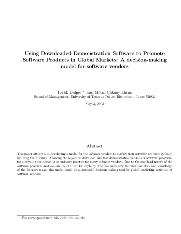
 Tevfik Dalgic