Image Recoloring Using Iterative Refinement

Image Recoloring Using Iterative Refinement ANDREI TIGORA Jinny Software Romania SRL 13 C Pictor Ion Negulici Primaverii, Bucharest Sector 1 ROMANIA andrei.tigora@jinnysoftware.com COSTIN-ANTON BOIANGIU Department of Computer Science and Engineering University “Politehnica” of Bucharest Splaiul Independentei 313, Bucharest, 060042 ROMANIA costin.boiangiu@cs.pub.ro Abstract: - This paper presents a new conversion algorithm from color images to grayscale that attempts to overcome the drawbacks of computing the grayscale luminance value as a weighted sum of the linear-intensity values. The algorithm aims to optimize the difference between neighboring color pixels based on the “potential” luminance difference. The algorithm iteratively adjusts the values associated to each of the pixel values, so that eventually there is a relevant difference between adjacent pixels so that the features become more visible. Key-Words: - Color to grayscale conversion, Color image processing, Dimensionality reduction, Iterative decolorization, image processing, color removal, information preserving color removal 1 Introduction Conversion from color to grayscale is a lossy process as it reduces a three-dimensional domain to a single dimension. The loss is an acceptable compromise that ensures compatibility with devices of limited capabilities or software that cannot handle the extra complexity associated with a three channel input. The main challenge is therefore creating an image that retains the core features of the original one, without introducing visual abnormalities. As human vision itself relies on luminance more than anything else, the most common procedure for grayscale conversion is weighted sum of the channel values that represent a particular color in the RGB model. While the end results are usually satisfactory, due to the fact that chroma and hue are completely ignored, some conversion scenarios have the potential of creating confusing outputs. To compensate for this drawback, modern algorithms usually add additional processing steps to the original grayscale conversion, aiming to optimize the result based on a previously defined evaluation function. A natural and information preserving conversion is useful for black and white typographies [6], document analysis, high performance binarization [7] or segmentation [9], local (adaptive) and global image processing [8], computer vision, as the algorithms usually receive as input grayscale images, which could end up being uniform using a standard color to grayscale algorithm. The rest of the paper is organized as follows. The next section is dedicated to related work. Section 3 contains the description of the algorithm we propose for grayscale conversion. The results and interpretation of the results are provided in Section 4, whereas the last section is reserved for conclusions and future work. 2 Related Work Based on how the pixels should be grouped, techniques for converting color images to grayscale can be roughly categorized as either global or local [4]. Global algorithms ensure that identical color pixels generate identical grayscale values. Local algorithms on the other hand, accomplish the conversion on small regions of the image, taking into consideration only the local features of those particular regions when applying the transformations. Whereas the algorithms in the first category are relatively fast, they offer poorer results than the ones based on local mapping. Yet, those in the latter category are way slower, due to the repetitive processing of overlapping regions, but produce better results. The classic conversion based on pixel luminance is perhaps the best example of global technique. Another classification splits the conversion methods into functional and optimizing [5]. Whereas functional conversions only rely on the actual pixel values to obtain the adequate gray scale pixel, optimizing methods also take into account more complex features than can only be obtained by analyzing the image as a whole. This classification, proposed by Benedetti et all [5], closely resembles the previous one, with the difference that it goes into more detail. Functional conversions can be further divided into trivial, direct methods and chrominance direct methods. Trivial methods either select a channel to represent the color, or average the values of the channels. Direct methods expand on the trivial ones, using weighted sums of the data channels. Chrominance direct methods aim to correct the results of direct conversion methods so that they better reflect human perception, as it illustrated by the Helmholtz-Kohlrausch effect. The optimizing methods vary greatly in their approaches[1], but they too can be classified into three groups. The first group consists of functional conversions that are then followed by various optimizations based on the characteristics of the image. The second employ iterative energy minimization, whereas the last category consists of various orthogonal solutions that do not fit within any of the previously enumerated categories. Information loss as result of the conversion is expected and unavoidable. Each of the techniques enumerated has its own advantages and disadvantages, and produces images that are best suited for a particular kind of processing (ex: contrast enhancing [2]) or just preserving the ambiance of the image [3]. The algorithm we propose is global, and its aim is directed primarily at converting human generated artificial RGB images that may become undistinguishable in grayscale. It should be noted though, that the algorithm is not limited strictly to a tridimensional color space, or the RGB color model. 3 Algorithm Description The input of the algorithm is an M  N matrix of vectors in the normalized RGB space, such that for each vector v , v  [0,1]3 . The output will be a M  N matrix of scalars, situated in the [0,1] range. Let there be three scalars  ,  ,  [0,1] ,      and       1 . In this context: - the module of vector v is | v |   x    y    z , where x , y and z uniquely correspond to red, green or blue - the virtual module of vectors v1 and v 2 is | v1, v 2 |   | x1  x 2 |    | y1  y 2 |    | z1  z 2 | - regarding relation  , it is said that v1  v2 if and only if | v1 || v2 or | v1 || v2 , x1  x2 or | v1 || v2 , x1  x2 , y1  y 2 or | v1 || v2 , x1  x2 , y1  y 2 , z1  z 2 - an optimum modulo difference of v1 and v 2 ( ) is defined as omd (v1, v 2) ( | v1, v 2 |  | v1 |  | v 2 |) / 2 if v1  v 2 and (| v1, v 2 |  | v1 |  | v 2 |) / 2 otherwise Step 1 The first step aims at initializing the data structures necessary for computation. Compute the modules of all vectors in the input matrix and store them in matrix A . ( M  1)  N of Compute matrix BV dimension, storing the optimum modulo differences of neighboring pixels, for the vertical direction. Similarly, compute the M  ( N  1) BH matrix storing the optimum modulo differences for the horizontal direction. All components situated on the edge rows (i.e. rows 0 and M ) of matrix BV and similarly the edge columns (i.e. columns 0 and N ) of BH respectively are 0 ; this is due to the fact that the original matrix is considered to be bordered with same value elements as those situated on the edge of the matrix. Create a map that uses as keys the encountered vector values in the matrix, and as corresponding value a structure that counts the identical vectors and a correction value. Step 2 For all entries in matrix A , evaluate the difference between neighboring element. That is, for i  1, M , | x |  | y | 1 j  1, N and compute x, y  {0,1,1} the , difference diff  A[i ][ j ]  A[i  y ][ j  x] . Extract this result from the value stored in either BH or BV that corresponds to the optimum modulo difference of the vectors situated at (i, j ) and (i  y, j  x) . This step attempts to determine how large the gap between the ideal difference and that stored in the matrix actually is, and use it to correct the situation. However, the correction is not applied directly; instead, the correction is added to the structure corresponding to the original vector that is stored at the same coordinates in the original matrix. For edge elements, because there is no neighbor element, the contribution for that particular element is equal to 0. Step 3 After all corrections have been accumulated, the correction is averaged to the number of vectors that contributed to the correction (the counter stored in the structure). The new correction is further decreased by a specified quota q then applied to all values in matrix A that correspond to the vector value group receiving the correction. The resulting value must be checked to prevent overflowing or under-flowing, therefore values are limited to [0,1] . The specified quota was introduced because changes in A tended to be radical and far from perfect, and left no place for improvement in future iterations. Step 4 The new configuration of matrix A is evaluated, and if it is better than the previous best alternative it is stored. An error index is computed based on how far neighboring elements in matrix A are from the neighboring ideals stored in BH and BV respectively. The error index is the sum of modulo differences between neighboring elements in matrix A and their corresponding values in either BH or BV If the newly computed error index is smaller than the previous best error index, then the current A matrix is a better approximation for the original matrix and the best matrix is updated. All corrections in the structures stored in the map are reset. If the upper limit of expected iterations has not been reached then Step 2 is run once again. 4 Results The test machine for the algorithm was an Intel Core2Duo, with 2GB of RAM running 64bit Windows7. The algorithm was written in C++ using Visual Studio. The algorithm was tested on two types of images: real-life photos and artificially generated. For real-life photos, there is little or no difference between the grayscale image obtained through simple transformations and the one obtained through the adaptive algorithm. This may be due to the fact that a particular pixel value has a wide range of neighboring values, which means that the applied correction is neither too high, nor too low. Another reason could be the actual number of existing values: there are so many pixel values within a reallife photo that even if some pixels are transformed, the overall impact on the image is negligible. 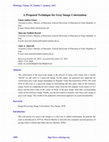Some results obtained in the “real-life photos” test scenario are presented in Fig. 1, where the proposed algorithm and the traditional grayscale conversion are presented side by side. 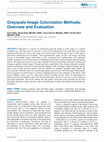Fig.2 Recoloring of artificial images: first row – original image, second row – grayscale image obtained through regular method, third row – grayscale image obtained through adaptive algorithm Fig.1 Recoloring of real-life photos: first row – original image, second row – grayscale image obtained through regular method, third row – grayscale image obtained through adaptive algorithm Although the results were satisfactory, the execution time was hardly so. Therefore, an attempt was made to reduce the execution time. Based on the experience from the development stages, it was decided that the quota q should not be a fixed one, instead it should be dynamically adjusted. The quota q starts at a maximum level q ; with each new 0 iteration, the value of q is decreased by a constant For the artificially created images on the other hand, the situation could not be more different. For specifically chosen images, the simple grayscale conversion algorithm creates images with a single tone of gray, whereas the adaptive algorithm conversion algorithm produces images with distinguishable elements. What is also interesting is that if new elements are added to a color image, and both the original and modified image are converted to grayscale, regions of the image that were unmodified in the color image can end up being different in the final grayscale image, as can be seen in the first and second row of images in Fig. 2. This is due to the fact that the new information propagates to all the regions of the image through the neighboring relations that are constantly evaluated. predefined reduction factor r . To prevent the quota from becoming too small, at each new iteration the number of resulting underflow and overflow values is counted and if it goes beyond a certain threshold T , q is reset to q 0 and the last iteration is repeated. Under normal circumstances there is no underflow or overflow. More significant though is the risk of having the changes become too “jumpy” and unpredictable, so a lower bound q1 , also has to be imposed on q . This lower bound allows for more free variation of the matrix values, but it is not so unpredictable to make recovery from an improbable path impossible. Following this change, visually, the resulting images were basically identical. From the mathematical point of view, there were slight differences between the images in the natural images, but within corresponding pixels, the difference was less than 1%. 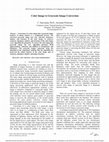As can be seen from Fig. 3, the average number of iterations drastically decreases by employing the dynamic quota. However, it did not go as low as it had originally been estimated. One reason is that in the later iterations the changes from one image to another are relatively slow, and hardly ever will influence the resulting integer based representation of the solution. This was especially true for the natural images, with high number of pixel values and high number of distinct neighboring pixel values. An attempt to set a threshold for the iterations that became increasingly less significant was made, but fixing a universally acceptable value did not produce improved results. Fig.3 Average number of iterations before obtaining the “ideal” image using the fixed and dynamic quotas 5 Conclusion and Future Work Future work will concentrate on finding a more efficient storage mechanism; perhaps instead of using a map entry for every single possible entry, a group of pixels could be considered similar enough and be evaluated together. Even so, the memory requirement for storing all possible values for a 24BPP image in a three dimensional matrix would require 16M structures, with an 4 octets for counter and 4 more for correction, this leads to a total of 256MB. Another aim would be to improve execution time by parallelizing the code; though for most of it this should be simple, the fact that the algorithm repeatedly updates the correction value can be a hurdle. On a completely different note, it would be interesting to modify the algorithm to take into account more than the difference between a pixel and its neighbors. Instead, the ideal reference matrix could be computed based on a smoothed matrix. A more radical approach would be to try a local based iterative solution. For that segmenting the image beforehand would be necessary, probably by intersecting sets of segmented areas for each of the channels. The regions that form the image would impose a correction on the neighboring regions which would result in corrections applied to the pixels that form the area. This could either be applied as a unique processing mechanism or in correlation with the global correction mechanism. References: [1] M. Ĉadík, Perceptual Evaluation of Colorto-Grayscale Image Conversions, Computer Graphics Forum, Vol. 27, 2007, pp. 17451754 [2] M. Grundland, N. A. Dodgson, Decolorize: Fast, contrast enhancing, color to grayscale conversion, Pattern Recognition, Vol. 40, No. 11, 2007, pp. 2891-2896 [3] A. Gooch, S. Olsen, J. Tumblin, B. Gooch, Color2Gray: salience-preserving color removal, Proceedings of SIGGRAPH '05, 2005, pp. 634-639 [4] M. Cui, J. Hu, A. Razdan, P. Wonka, Color to Gray Conversion Using ISOMAP, The Visual Computer, Vol. 26, No. 11, pp. 1349-1360 [5] L. Benedetti, M. Corsini, P. Cignoni, M. Callieri, R. Scopigno, “Color to gray conversions in the context of stereo matching algorithm: An analysis and comparison of current methods and an adhoc theoretically-motivates technique for image matching”, Machine Vision and Applications, Vol.23, No. 1, pp. 327-348 [6] Costin-Anton Boiangiu, Ion Bucur, Andrei Tigora “The Image Binarization Problem Revisited: Perspectives and Approaches”, The Proceedings of Journal ISOM Vol. 6 No. 2 / December 2012, pp. 419-427 [7] Costin-Anton Boiangiu, Andrei Iulian Dvornic. “Methods of Bitonal Image [8] Conversion for Modern and Classic Documents”. WSEAS Transactions on Computers, Issue 7, Volume 7, pp. 1081 – 1090, July 2008 Costin-Anton Boiangiu, Alexandra Olteanu, Alexandru Victor Stefanescu, Daniel Rosner, Alexandru Ionut Egner (2010). „Local Thresholding Image Binarization using Variable-Window Standard Deviation Response”, Annals of DAAAM for 2010, Proceedings of the 21st International [9] DAAAM Symposium, 20-23 October 2010, Zadar, Croatia, pp. 133-134, Vienna, Austria 2010 Costin-Anton Boiangiu, Dan-Cristian Cananau, Bogdan Raducanu, Ion Bucur, “A Hierarchical Clustering Method Aimed at Document Layout Understanding and Analysis”, International Journal of Mathematical Models and Methods in Applied Sciences, Issue 1, Volume 2, 2008, Pp. 413-422