An experimental and CFD study of liquid jet injection into a partially baffled mixing vessel: A contribution to process safety by improving the quenching of runaway reactions

Chemical Engineering Science 63 (2008) 924 – 942 www.elsevier.com/locate/ces An experimental and CFD study of liquid jet injection into a partially baffled mixing vessel: A contribution to process safety by improving the quenching of runaway reactions Jean-Philippe Torré a,b,c , David F. Fletcher b,∗ , Thierry Lasuye c , Catherine Xuereb a a Laboratoire de Génie Chimique, Université de Toulouse, CNRS/INP/UPS, Toulouse, France b School of Chemical and Biomolecular Engineering, The University of Sydney, NSW 2006, Australia c LVM Quality and Innovation Department, Usine de Mazingarbe, Chemin des Soldats, 62160 Bully Les Mines, France Received 9 August 2007; received in revised form 25 September 2007; accepted 22 October 2007 Available online 30 October 2007 Abstract Thermal runaway remains a problem in the process industries with poor or inadequate mixing contributing significantly to these incidents. An efficient way to quench such an uncontrolled chemical reaction is via the injection of a liquid jet containing a small quantity of a very active inhibiting agent (often called a stopper) that must be mixed into the bulk of the fluid to quench the reaction. The hazards associated with such runaway events mean that a validated computational fluid dynamics (CFD) model would be an extremely useful tool. In this paper, the injection of a jet at the flat free surface of a partially baffled agitated vessel has been studied both experimentally and numerically. The dependence of the jet trajectory on the injection parameters has been simulated using a single-phase flow CFD model together with Lagrangian particle tracking. The comparison of the numerical predictions with experimental data for the jet trajectories shows very good agreement. The analysis of the transport of a passive scalar carried by the fluid jet and thus into the bulk, together with the use of a new global mixing criterion adapted for safety issues, revealed the optimum injection conditions to maximise the mixing benefits of the bulk flow pattern. 䉷 2007 Elsevier Ltd. All rights reserved. Keywords: Mixing; Agitated vessel; Quenching; Thermal runaway; CFD; Jet injection 1. Introduction Many reactions within the process industry are exothermic. In batch or semi-batch reactors when the heat generated by chemical reaction exceeds that removed by cooling, an uncontrolled increase of temperature can occur. This loss of control is termed a thermal runaway. Balasubramanian and Louvar (2002) used several government and private sectorsafety-related databases, in addition to other published safety resources, to review major accidents and summarised some lessons learned. The authors revealed, by determining the number of runaways resulting in a major incident in the chemical industries, that 26.5% of the major accidents in the petrochemical industries for the 40-year period from 1960 to 2000 were ∗ Corresponding author. Tel.: +61 2 9351 4147; fax: +61 2 9351 2854. E-mail address: d.fletcher@usyd.edu.au (D.F. Fletcher). 0009-2509/$ - see front matter 䉷 2007 Elsevier Ltd. All rights reserved. doi:10.1016/j.ces.2007.10.031 the result of runaway reactions. Butcher and Eagles (2002) declared that on average around eight runaway incidents a year occurred in the UK, with poor mixing being a significant contributor to these incidents. More precisely, an analysis of Barton and Nolan (1989) of 189 incidents which occurred in industrial batch reactors in the UK chemical industry between 1962 and 1987 revealed that polymerization reactions account for almost 50% of the classified incidents for which there was a high potential for loss of control and runaway. In addition, the Health and Safety Executive reported that for Great Britain in the four year period from 1994 to 1998, 203 incidents involving exothermic runaway or thermal decompositions occurred, with the majority of these being due to the inadvertent mixing of chemicals (Fowler and Hazeldean, 1998; Fowler and Baxter, 2000). As analysed by Westerterp and Molga (2004), most of these runaway events caused at best loss and disruption of production and perhaps equipment damages, at worst they had J.-P. Torré et al. / Chemical Engineering Science 63 (2008) 924 – 942 the potential for a major accident and could affect not only the reactor itself but also represent a hazard for plant workers and the surrounding plant. Despite the fact that much progress has been made to understand and limit such runaway reactions, this problem still occurs. According to Westerterp and Molga (2006), three “lines of defence” have to be considered to prevent a reactor incident: (a) the choice of the right operating conditions, (b) an early warning detection system, and (c) a suitable system to handle runaway reactions. Although the prevention of such accidents requires detailed knowledge of the reaction process, the “two first lines of defence” (items (a) and (b)) have received considerable attention (Etchells, 1997; Gustin, 1991; McIntosh and Nolan, 2001; Westerterp and Molga, 2006; Zaldívar et al., 2003) over the last 30 years following the accident that occurred in Seveso (Italy) in 1976, and are not discussed further here. Concerning the quenching of an exothermic reaction once the runaway is in progress, an efficient process to avoid runaway is the injection and the mixing of a small quantity of an efficient inhibiting agent (also called a “stopper” or “killer” in the polymer industry) into the bulk. This inhibition process is often associated with important mixing problems (McIntosh and Nolan, 2001). Particularly, the problem is worse after a breakdown of the agitation system (Torré et al., 2007b; Platkowski and Reichert, 1999) due to the poor mixing which results from a decreasing agitation speed. The mixing of small quantities of very active substances in free-radical-initiated reaction systems, such as for polymerisations products, foaming mixtures or highly viscous fluids, requires an injection system with optimal design and efficiency. Experimental studies which couple the quenching efficiency of the “killer” and hydrodynamics of both the stirred vessel and the injection system are rare in the literature. Kammel et al. (1996) studied jet tracer injection into a non-agitated vessel with model fluids and found that the mixing time, tm95% , was dependent on the jet Reynolds number (Rej = vj dj j /j ) and the filling ratio of the vessel. Related to jet injection, extensive research has also been undertaken to understand the physical phenomena that control by-product formation via competitive or consecutive reactions, conducted in turbulent mixing conditions. Although experiments are carried out with very low feed velocities, leading to laminar flow in the feed pipes, the studies of Baldyga et al. (1993) or Bałdyga and Pohorecki (1995) discuss the processes of micro, meso and macromixing in the vessel where the flow is turbulent. Concerning high velocity feeds, Verschuren et al. (2001) provided a method for the calculation of the time-scale of turbulent dispersion of the feed stream introduced inside a stirred vessel. Recently, Bhattacharya and Kresta (2006) used a mixing-sensitive chemical reaction to analyse the effects of the feed time and the jet velocity on the performance of a reactor fed with a high velocity surface jet. They suggest that rapid convection of the reagents from the surface to the impeller swept region can potentially improve the performance but that experimental and theoretical analysis has revealed otherwise. Due to the hazards linked to thermal runaways, laboratory and pilot-plant scale experiments in runaway conditions are difficult to carry out, thus the use of computational fluid dynamics 925 (CFD) is extremely useful. Several authors have used CFD to study the mixing of an inhibiting agent in a stirred vessel. Balasubramanian et al. (2003), Dakshinamoorthy et al. (2004, 2006) and Dakshinamoorthy and Louvar (2006) showed CFD to be a powerful tool in the quest to understand the mixing of an inhibiting agent in an agitated vessel, as it can be used to study the effect of different injection positions and the quantities of inhibitor introduced. For a fully baffled stirred vessel, they extended the hydrodynamics study, using a multiple reference frame (MRF) approach, to simulate in transient conditions the instantaneous runaway and inhibition reactions by coupling the reaction kinetics equations (for propylene oxide polymerisation) with the flow and transport equations. In the CFD model developed, the entire volume of inhibiting agent was added instantaneously to a part of the tank, and then the transport equations were solved in a transient manner. As stated by the authors in Dakshinamoorthy et al. (2004), this assumes that the addition of stopper does not influence the fluid dynamics inside the stirred vessel. A complete description of the different inhibition systems and the possible alternatives is reviewed by McIntosh and Nolan (2001) and is not repeated here. Although a jet injected at the surface of a stirred vessel can be used to quench an uncontrolled reaction for many reaction mixtures, McIntosh and Nolan (2001) highlighted that one of the main reasons that this system is not popular for industrial applications, despite its efficacy, is the lack of published information concerning the injection system, together with uncertainties over the mixing efficiency and distribution of the inhibitor within the bulk. Bhattacharya and Kresta (2006) concluded that the behaviour of a feed stream with more momentum than the ambient fluid is largely unknown, compounding the problems of this approach. In contrast, the stability and fragmentation of liquid jets has been studied extensively over the past 170 years. Since the earliest investigations into jet flow phenomena, which appear to have been carried out by Bidone (1829) and Savart (1833), many studies have been performed on jet hydrodynamics, as reviewed by McCarthy and Molloy (1974). As a detailed analysis of jet theory is not the aim of this paper, the reader can consult Rajaratnam (1976) and more recently Pope (2000) and Sallam et al. (2002) for reviews of experimental results and theoretical developments concerning turbulent jets. Surprisingly, no studies were found in the literature concerning the trajectories of a fluid jet injected at the free surface of an agitated vessel for batch operation. The CFD study, complemented by experimental investigation, presented in this paper examines fluid injection via a jet on a flat free surface of a partially baffled stirred vessel designed for industrial polymer synthesis applications. CFD and experimental hydrodynamics studies, together with numerical predictions of the free surface shape, have been carried out without considering jet injection for the same vessel in our previous work (Torré et al., 2007a,b,c). A single-phase flow model, in which the inhibiting agent is represented as a fluid with the same density and viscosity as the fluid in the tank, that tracks the injected fluid via its concentration is developed. In addition, neutrally buoyant particles are released at the jet inlet to allow 926 J.-P. Torré et al. / Chemical Engineering Science 63 (2008) 924 – 942 visualisation of the jet trajectory in a Lagrangian manner. This modelling approach takes into account the modification of the hydrodynamics of the bulk during the inhibitor injection via the momentum of the injected jet. Simulations covering various jet cross-sections and jet velocities allow the quantification of the jet trajectory following injection. The predicted jet profiles are compared with experimental data for the penetration of the fluid into the bulk. Then, the concept of a global mixing criterion is defined to quantify the mixing quality and to assess the influence of the jet trajectory on the quenching efficiency. 2. Experimental apparatus The experiments carried out for this study have been conducted in a pilot reactor designed for polymer and fine chemicals industrial applications. To carry out hydrodynamics studies with the possibility of injecting additives, this reactor is composed of two different sections: the liquid injection system and the agitated vessel. The complete apparatus is shown in Fig. 1 and the main dimensions are presented in Table 1. The liquid injection system consists of a 3 l high pressure (max 125 bars) steel vessel manufactured by Hoke (commonly called a “sampling cylinder” because it is used to take a fluid sample from a chemical process unit and store it safely for future analysis). This vessel, of diameter and height equal to 102 and 559 mm, respectively, has two orifices of 15 mm diameter each located at the top and bottom. The top orifice is fitted with a four junction piping element which is used: (i) to mount a steel funnel (isolated from the vessel by a manual valve) to feed the liquid, (ii) to feed the air to pressurise the vessel, (iii) to mount a pressure sensor (Keller, model PR21/10b) and (iv) to mount a safety relief valve. A constant pressure reducing valve located on the air feed pipe is used to maintain a constant pressure in the vessel during draining. A high-speed automatic valve controlled via a pneumatic actuator (using air at 8 bars) is mounted directly at the bottom of the vessel. A 15 mm diameter passage with no obstruction exists when the valve is open. The liquid volume present initially in the vessel is introduced into the stirred vessel via different single tubes located at Xj = −94 mm and Zj = 129.4 mm from the reactor central axis, as shown in Fig. 1(b). The liquid jet impacts directly on the free surface of the stirred liquid and the pipe outlet is located at a distance, L′ , of 220 mm above the liquid free surface for all the experiments. Three different injection pipes (internal diameter, d, equal to 7.2, 10 and 15 mm) with the same total pipe length (L = 300 mm) are used for the experiments carried out in this study. The ratio L/d takes values up to 20, giving fully developed turbulent conditions at the pipe outlet. Fig. 1. Details of the mixing vessel and its injection system: (a) side view; (b) top view; (c) details of the impeller. J.-P. Torré et al. / Chemical Engineering Science 63 (2008) 924 – 942 Table 1 Geometrical dimensions of the vessel and the injection system Tank diameter Maximum tank height Bottom dish height Agitator diameter Number of agitator blades Agitator blade width Agitator blade thickness Agitator retreat angle Agitator clearance Baffles length Number of baffles Baffle width Baffle thickness Distance baffle–shell Initial liquid height Injected volume Injection pipe diameter Injection pipe length Distance pipe outlet–free surface Jet injection location on the X axis Jet injection location on the Z axis Symbol Value T Hmax Hd D nb wb tb 450 mm 1156 mm 122.9 mm 260 mm 3 58 mm 9 mm 15◦ 47.2 mm 900 mm 2 46 mm 27 mm 38.5 mm 700 mm 533 ml 7.2, 10, 15 mm 300 mm 220 mm −94 mm 129.4 mm  C Bl nB BW Bt B′ Hliq Vj d L L′ Xj Zj The agitated vessel is a partially baffled reactor equipped with a bottom entering agitator system inside a steel curved bottom dish. Two beaver-tail baffles are suspended from the top lid. The agitator is a three blade impeller, derived from the classical retreat blade impeller (RBI) developed by Pfaudler but this model has a larger blade width. The impeller rotates in the anti-clockwise sense and its geometry is presented in Fig. 1(c). The filling ratio of the vessel is maintained constant in all the experiments and the height of water at ambient temperature is fixed at 700 mm. For further details of this mixing equipment, the reader can consult Torré et al. (2007a). The tracking of the liquid jet during its penetration into the agitated liquid after impact with the free surface required the use of a high resolution CMOS camera, UV lighting and Fluorescein. The high-speed camera used is a HCC-1000 model from VDS Vossküler, monitored using the NV1000 software from New Vision Technologies. The camera is equipped with a tele-zoom lens (Rainbow S6X11) having an 11.5–69 mm focal length, and 1:1.4 maximum relative aperture. The frame rate, exposure time and picture resolution are 51.44 frames per seconds, 15.2 ms and 1024 × 1024 pixels2 , respectively, and these settings remained the same for all of the experiments. The UV light used to illuminate the jet trajectory is produced by two “blacklight” tubes (Philips TL-D, 120 mm length, 26 mm diameter, max =355 nm) of 36 W each. The UV tubes were mounted vertically in front of the vessel to cover the entire height of the transparent vessel shell, as shown in Fig. 1(b). The Fluorescein (formula: C20 H10 O5 Na2 , molecular weight: 376.28 g/mol) used for preparing the aqueous solutions of the injected liquid is a disodium anhydrous salt of general purpose grade provided by Fisher Scientific. This molecule is a commonly used fluorofore which has absorption and emission maxima at 494 and 521 nm (in water), respectively. 927 3. CFD model The numerical simulations were performed using ANSYSCFX 11.0, which is a commercial CFD package that solves the Navier–Stokes equations via a finite volume method and a coupled solver. The equations used in the modelling are given in Appendix A. An unstructured mesh composed of prismatic, tetrahedral and pyramidal elements was used and the boundary layer resolution was increased by using inflation meshing at all walls. A region of fine mesh below the jet injection point and descending to 500 mm below the inlet surface was used to ensure the accurate capture of the jet trajectory. The final grid used for this modelling, presented in Fig. 2, was composed of 293,000 nodes (1,313,000 elements). The refinements of the grid in the jet injection region were made to the grid used in our previous work, where the density of cells was optimised previously to resolve the flow in the vessel (Torré et al., 2007a,b,c). The mixing of the jet in the stirred vessel is investigated via transient simulations using Eulerian and Lagrangian approaches simultaneously. We use two different approaches because we want to avoid numerical diffusion errors in tracking the path of the jet, for which Lagrangian particle tracking is well-suited, and we inject a scalar concentration to look at the global mixing behaviour because it is impractical to inject enough particles to generate a smooth concentration field that can be used in a meaningful way to compare different injection conditions. The agitated fluid is water at 25 ◦ C ( = 997 kg m3 and  = 8.9 × 10−4 Pa s) and the inhibiting agent is represented as a fluid with the same density and viscosity as the fluid in the tank. The concentration of the injected fluid is tracked by solving an additional non-reacting scalar transport equation. The mass fraction of the passive scalar at injection was set to one. We have used a non-reacting scalar as the process of interest is mixing-limited rather than being controlled by the availability of the added fluid because the mass of “stopper” injected is more than sufficient to quench the reaction throughout the tank. We recognise that when simulations of an industrial system are made for a specific process a reactive scalar should be used. In parallel, neutrally buoyant particles were released at random locations from the inlet in order to visualise the jet trajectory during the injection time. These marker particles were given a small diameter (10 m) and the Schiller Naumann drag law was used so that they would follow the mean flow of the injected fluid. A turbulent dispersion force, derived from an eddy interaction model, was added to model the turbulent fluctuations which affect the tracer particle trajectory when the ratio of the eddy viscosity to the dynamic fluid viscosity is above five (ANSYS-CFX 11.0, 2007). As the particles do not affect the flow field, the fluid–particle interaction is treated via one-way coupling, so that the particle path was updated at the end of each time-step. Lagrangian particles were released from two different randomly located positions per timestep, and the timestep was set to 1 ms for all runs. The injection rate of particles was based on an assessment of the number needed to properly visualise the jet trajectory without adding so many that the computations became two slow and demanding in memory. 928 J.-P. Torré et al. / Chemical Engineering Science 63 (2008) 924 – 942 Fig. 2. The mesh used for the CFD simulations: (a) vertical plane passing through the centre of the injection surface; (b) details of the mesh on the agitator and (c) on a baffle. The timestep value was chosen such that convergence of the residuals was achieved in less than five coefficient loops. The agitator rotation speed was maintained at a constant value of 100 RPM in the base case simulations (giving a Reynolds number of 1.3 × 105 ) and was subsequently varied between 50 and 150 RPM. At these rotation speeds, the experiments and CFD modelling using an inhomogeneous multiphase model have shown that the free surface is quasi-flat with a small precessing vortex which rotates on the free surface around the vessel axis (Torré et al., 2007c). The injected volume (always equal to 533 ml) leads to an increase of the water level of less than 4 mm which is negligible compared with the 700 mm of the initial water height and therefore the increase of the free surface level following fluid injection was neglected. Therefore, the use of a multiphase model to predict the free surface deformation was not necessary at the agitator rotation speeds considered here and the inlet used for jet injection was located directly on the free surface. The authors previously used the sliding mesh (SM) model to study the same partially baffled vessel used here in order to determine the complex, time-dependent hydrodynamics and transient effects, which consisted of multiple recirculation loops and macro-instabilities (Torré et al., 2007c). The need to study numerous jet injection conditions and to run the simulations for 18 s of real time meant that the MRF model was preferred to the SM model, which was considered to be too computationally demanding for this work. The MRF model has been shown to perform well for this configuration (Torré et al., 2007a). Therefore, a rotating reference frame is applied to the bottom dish and a stationary frame is applied to the cylindrical part of the vessel which contains the baffles, with these frames joined via a frozen rotor condition. We note that this is a major simplification but it would be extremely computationally demanding and difficult to analyse the results if we included the transient rotation of the impeller. Our previous work has shown that at least 15 revolutions of the impeller must be made for a transient simulation that starts from a steady-state simulation to be meaningful. As we wanted to look at many jet locations and conditions we decided to pursue the strategy of interacting the jet with a mean flow-field obtained from a frozen rotor approach, in which a transient simulation was performed but the impeller blade was not rotated. In Torré et al. (2007c) we noted that the time-averaged transient results show a similar flow structure to the steady-state results. In addition, the transient model captures the free surface behaviour well, as the steady-state model does at higher rotation speeds. Based on these observations we felt justified in using the frozen rotor approach in this study. J.-P. Torré et al. / Chemical Engineering Science 63 (2008) 924 – 942 A no-slip boundary condition is imposed on the agitator, the baffles, the bottom dish and the vessel shell. An inlet boundary condition is specified for the jet injection surface with a specified mass flow of injected liquid. This allows a fixed volume (533 ml) of liquid, which enters the stirred vessel with a known momentum flux, to be applied only during the injection time. The jet momentum flux, denoted by M, is defined as the product of the liquid jet density, the jet cross-sectional area and the square of the jet velocity. The entire top surface of the vessel, excluding the injection area, is set as a free-slip surface with a mass sink applied at the surface to remove the same volume of fluid as injected at the inlet, thus maintaining the liquid level constant. The choice of the turbulence model was determined based on a previous paper (Torré et al., 2007c) through comparisons between experimental PIV data and numerical predictions. The SSG Reynolds stress model gave unphysical results for axial velocities in the areas close to the vessel axis, whilst the standard k. turbulence model showed good agreement with experimental PIV data and captured the shape of the free surface well. Thus, the standard k. turbulence model, together with the scalable wall function treatment available in ANSYS CFX (Grotjans and Menter, 1998), was used in this study. A second order bounded spatial differencing scheme was used to limit numerical diffusion as much as possible and second order time integration was performed. A maximum number of 10 coefficient loops per time step was sufficient to decrease the normalised RMS residuals below 10−4 for the mass, momentum, turbulence and the passive scalar transport equations, with this value being considered sufficient to have a converged simulation (ANSYS-CFX 11.0, 2007). 4. Experimental trajectories of the liquid jet 4.1. Jet velocity The jet velocity was measured experimentally on the pilot reactor for different operating conditions. With the injection system used in this study, the jet velocity is controlled by the air pressure in the steel vessel which contains the liquid to be injected. In all the experiments carried out the steel vessel was filled with 0.533 l of tap water, leaving an air space volume of about 2.5 l above the liquid surface under pressurised conditions. For the experiments conducted at atmospheric pressure (P = 0), the valve of the feeding funnel remained open allowing an outlet to the atmosphere. For the other pressures tested (P > 0), the pressure reducing valve located on the air feed pipe of the steel vessel allowed a constant pressure to be maintained inside the steel vessel. The experiments were carried out with three different injection pipe diameters, equal to 7.2, 10 and 15 mm. The pressure in the steel vessel was set from 0 to 2 bars to cover a large range of jet velocities. The shape of the free-falling liquid jet was captured using the high-speed camera with a frame rate of 463 fps and with an exposure time of 2.16 ms, and using a calibration (1 pixel on a picture corresponded to a distance of 0.1446 mm). The jet velocity was deduced from the 929 measurement of the displacement of the jet leading edge for the maximum number of frames, for which the jet leading edge was visible. Although the leading edge of the jet bulges as it descends, due to the drag effect of the air on the liquid, the jet remained coherent for all the jet diameters, velocities and liquid fall distances used in this study. Fig. 3(a) shows the evolution of a water jet released at atmospheric pressure into the air space above the free surface of the stirred liquid. The rounding of the leading edge of the jet is clearly visible and the precision of the determination of the jet position was assumed to be 5 pixels. From these pictures, the leading edge of the jet travelled a distance of 109.6 mm in 0.0518 s which corresponds to a jet velocity of 2.11 ± 0.03 m s−1 . For each set of parameters tested, the final jet velocity (used for further calculations) was calculated as the arithmetic average of five measurements obtained during different experiments. The results are presented in Fig. 3(b), where each velocity value has been plotted versus the absolute pressure inside the steel vessel for the three pipe diameters tested. The errors bars are equal to the standard deviation (±) of five experimental measurements. In the analysis that follows it is assumed that the initial jet velocity is representative of the average jet velocity during the entire injection time. Using the video recording method described earlier, it was not possible to track the front of the jet at the end of the injection time due to the gas/liquid mixture expelled by the gas. 4.2. Experimental jet trajectories The problem of a free-falling liquid jet which impacts a liquid surface has received considerable attention in the literature, with most studies focussed principally on the gas entrained into the quiescent liquid (Bin, 1993; El Hammoumi et al., 2002; McKeogh and Ervine, 1981). As concluded by Bin (1993) and reported by Chanson et al. (2004), the mechanism of air entrainment depends upon the jet impact velocity, the physical properties of the liquid, the nozzle design, the length of the freefalling jet and the jet turbulence level. In the experiments carried out in this study, the injection conditions were such that air was always introduced in the liquid present in the stirred vessel. Nevertheless, this study differs from classical free-falling jet studies as the main purpose is not to study the gas introduction but to quantify experimentally the liquid jet trajectory during its penetration into the bulk. Fig. 4 shows a typical jet, captured using the black and white camera with classical daylight conditions. For this experiment a volume of 533 ml of water, added to 10 ml of iodine aqueous solution at 1 mol/L used as a dye, was injected into the partially baffled vessel during agitation. It is obvious that the dark jet plume visible in Fig. 4(a) during injection is a gas–liquid mixture. Air is entrained due to interfacial shear at the liquid jet interface, which drags down an air boundary layer, and due to the air entrapment process at the point of impact (Davoust et al., 2002). Thus, air bubbles are entrained by the jet, then detach and finally reach the free surface due to buoyancy, as is clearly visible in Fig. 4(b). The air bubbles entrained with the injected liquid create a dark 930 J.-P. Torré et al. / Chemical Engineering Science 63 (2008) 924 – 942 Fig. 3. (a) Snapshots of a water jet released in air obtained with d = 10 mm and V = 2.1 m s−1 ± 0.1 (P = 0 bar); (b) jet velocities versus the pressure measured in the sampling cylinder for three injection pipe diameters (7.2, 10 and 15 mm), symbols: arithmetic average of 5 experiments, error bars: ±. Fig. 4. Visualisation of a water jet coloured with iodine, injected at the free surface with classical daylight conditions (d = 10 mm, V = 6.0 ± 0.5 m s−1 , N = 100 RPM): (a) during injection; (b) after injection. air–water interface, which prevents accurate visualisation of the liquid jet trajectory inside the stirred vessel. Thus, this method is well adapted to visualise the gas bubbles and the gas/liquid two-phase region but is not appropriate for tracking the injected liquid with any degree of accuracy. A possible means to track the liquid jet is a method that highlights the injected liquid without showing the air bubbles. To make this possible an aqueous solution of Fluorescein with a concentration of 0.2 g/l has been used for the injected liquid. The vessel was lit by UV light and the jet injection was recorded with the same black and white camera without any other light in the room. This approach has two main advantages for the present study: (a) injection of an aqueous solution of Fluorescein is very easy to track because this appears as a bright yellow liquid under UV light, (b) the air bubbles are invisible under UV. Point (b) was demonstrated experimentally by injecting air at various flow rates below the agitator in the stirred vessel filled with tap water. Three experiments have been carried out for each set of parameters tested. Recording each experiment with a high-speed camera allowed tracking of the jet penetration trajectories from the beginning to the end of jet injection. The time at the end of injection is denoted Tinj , and the times equal to 0.2Tinj , 0.4Tinj , 0.6Tinj , 0.8Tinj and Tinj have been considered for the jet trajectories, and for subsequent comparisons with the numerical data. Example experimental jet snapshots at time Tinj are presented in Figs. 5. The three raw pictures have been transformed so that each has one of the three primary colours (red, green and blue) of equal intensity, as shown in Figs. 5(a), (b) and (c). Then, for ease of comparison with the numerical jet trajectory predicted by CFD and to quantify the reproducibility of the experiments, an RGB imaging process (additive synthesis of colours) was used to compile them into a single final picture using the software IRIS. The common area of the three different pictures is white on the final frame, as presented in Fig. 5(d). The hydrodynamics in this partially baffled vessel are very complex (Torré et al., 2007c). In short, the liquid circulation consists of a downward stream in the centre of the vessel and an upward stream at the periphery, with a rotational flow superposed on these streams. This partially baffled vessel is fitted with only two beaver-tail baffles so that the baffling effect is not sufficient to break the strong tangential motion imparted by the agitator (rotating counter-clockwise). At the same time as the jet expands its diameter radially, its velocity decreases and the jet fluid is entrained by the stirred fluid leading to the bending of the jet plume, as shown in Fig. 5. The jet is then J.-P. Torré et al. / Chemical Engineering Science 63 (2008) 924 – 942 931 Fig. 5. Snapshots at the end of the injection time obtained using a Fluorescein aqueous solution lit with UV and their superimposition via the RGB imaging process: (a) first experiment, red component of the RGB picture; (b) second experiment, green component of the RGB picture; (c) third experiment, blue component of the RGB picture; (d) RGB final picture. The conditions were d = 10 mm, V = 6 m s−1 , N = 100 RPM. dispersed in the vessel due to two turbulent mechanisms: the dispersion of the plume by small eddies with a size equivalent to the size of the plume and the fluctuation of the entire plume around its mean position due to large-scale turbulent motions (Verschuren et al., 2002). A very important point that must be noted about this study concerns the introduction of air bubbles in the vessel during the injection, as shown in Fig. 4. These bubbles enhance mixing in the vicinity of the jet, deform the jet plume and create turbulence because of the rise of the bubbles due to buoyancy. As shown in Figs. 5(a)–(c), some fluorescent tracer is entrained by the air bubbles from the jet plume to the surface. This increases the liquid jet dispersion and makes the jet plume appear larger compared with the same experiment carried out with a plunging pipe. The dynamics of disengagement of the entrained air bubbles differs from one experiment to another, depending on the flow structure which exists in the vessel during the jet injection. This chaotic phenomenon, added to the high unsteadiness of the flow (e.g. precessing vortex, macro-instabilities) which develops in the stirred vessel (Torré et al., 2007c), makes the jet trajectory non-reproducible from one experiment to the next. The non-reproducibility is shown by the coloured areas of Fig. 5(d), where the contribution of the air bubbles rising is clear at the edge of the visible plume. In contrast, few coloured areas are noticeable in Fig. 5(d) near the lower limit of the jet plume, which demonstrates that the lower penetra- tion limit is almost identical in the three experiments carried out. Tracking the jet trajectory experimentally in an agitated vessel is very complex due to the 3D nature of the flow. Another difficulty is the unsteadiness of the injection which adds to the transient effects of the flow in the stirred vessel. Concerning this latter point, the problem must be considered in a different way to that of feeding studies carried out in continuous stirred tanks reactors (CSTR), such as those presented in Aubin et al. (2006), in which the determination of the jet trajectory is easier. The visualisation of the jet mixing with only one camera located in front of the vessel does not record the real 3D movement of the injected liquid but allows analysis of the projection of this trajectory onto a plane. Therefore, CFD simulations were developed to analyse qualitatively the jet trajectory for several jet conditions (diameter and velocity) and to quantify the mixing process in the entire agitated vessel. 5. CFD predictions of the jet trajectories The modelling of the trajectory of the liquid jet has been carried out for various injection conditions at a constant agitator speed (N = 100 RPM). Nine simulations were analysed, involving three jet diameters (7.2, 10 and 15 mm) and three jet velocities (2, 6 and 10 m s−1 ), to quantify the effect of the injection parameters on the liquid jet trajectory and its penetration into the stirred vessel for N =100 RPM. Using the physical 932 J.-P. Torré et al. / Chemical Engineering Science 63 (2008) 924 – 942 Fig. 6. Lagrangian jet trajectories coloured by the Lagrangian particle travel time normalised by Tinj , for d = 7.2 mm, V = 2 m s−1 and N = 100 RPM, plotted at 0.2Tinj , 0.4Tinj , 0.6Tinj , 0.8Tinj and Tinj : (a) 3D view; (b) XY lateral view; (c) Y Z lateral view; (d) top view. J.-P. Torré et al. / Chemical Engineering Science 63 (2008) 924 – 942 933 Fig. 7. Lagrangian jet trajectories coloured by the Lagrangian particle travel time normalized by Tinj , for d = 10 mm, V = 10 m s−1 and N = 100 RPM, obtained at 0.2Tinj , 0.4Tinj , 0.6Tinj , 0.8Tinj and Tinj : (a) 3D view; (b) XY lateral view; (c) Y Z lateral view; (d) top view. 934 J.-P. Torré et al. / Chemical Engineering Science 63 (2008) 924 – 942 Fig. 8. Lagrangian particle tracking (300 particles) showing the jet penetration profile (d = 10 mm, V = 6 m s−1 ) at the end of the injection time for different agitator rotation speeds, coloured with the normalised vessel height H ∗ (=Y /Hliq ): (a) N = 50 RPM; (b) N = 75 RPM; (c) N = 100 RPM; (d) N = 125 RPM; (e) N = 150 RPM. properties of water at 25 ◦ C, these parameters gave jet Reynolds numbers which varied from 1.61 × 104 (d = 7.2 mm and V = 2 m s−1 ) to 1.68 × 105 (d = 15 mm and V = 10 m s−1 ) all giving fully turbulent jet conditions. All of the jet trajectories are not presented here and only two relevant examples of different jet profiles are detailed. With four different geometrical views (3D, two laterals and top), Figs. 6 and 7 provide a good qualitative description of the jet behaviour in the stirred vessel. The trajectory is shown using the tracks of the Lagrangian particles at different times during the injection, with the number of particles being proportional to the injected volume. Therefore, 60, 120, 180, 240 and 300 Lagrangian particles have been used to visualise the jet trajectory at the times 0.2Tinj , 0.4Tinj , 0.6Tinj , 0.8Tinj and Tinj , respectively. Fig. 6 shows the behaviour of a 7.2 mm liquid jet diameter, injected with a velocity of 2 m s−1 into the stirred vessel. As shown in Figs. 6(b) and (c), these conditions lead to very little downward jet penetration, and the deflection of the jet plume occurs close to the free surface. The circumferential movement of the stirred fluid is sufficient to entrain the injected fluid rapidly into the central vessel region. The region near the vessel axis is characterised by a highly swirling movement with significant streamline curvature (Torré et al., 2007a,c), so that the injected liquid is pulled downwards. It is then pumped axially and expelled radially by the agitator, with the injected fluid then being deflected by the bottom curved dish and subsequently it flows upwards close to the vessel wall. In contrast with the case presented above, Fig. 7 shows a very different injection behaviour characterised by a higher jet velocity and a larger jet diameter. As shown in Figs. 7(b) and (c), these injection parameters are such that the injected fluid penetrates vertically much deeper into the bulk before the jet plume becomes entrained by the tangential movement of the stirred liquid. The analysis of the nine simulations revealed that the vertical penetration of the jet increases with both the jet diameter and the jet velocity. No correlations were found in the literature relating to the behaviour of jet trajectories penetrating into a stirred vessel, probably due to the difficulty of describing the jet movement in a 3D, rotating flow which have a variable axial component along the jet axis. The theoretical analysis which appeared to be the closest to the case studied here is that for liquid jets injected into a cross-flow. As mentioned in Muppidi and Mahesh (2005), the dependency of the mean jet trajectory on the jet diameter is well-known and the flow field of a jet in a cross-flow is believed to be influenced primarily by the effective velocity ratio R (which in this case simplifies to R = uj /ucf , where uj is the jet velocity and ucf is the cross-flow velocity). Therefore, although the jet trajectory is not explained here in detail, the results obtained are in agreement with those found for a jet in a cross-flow. Four additional simulations have been carried out to determine how the jet trajectories behave at different agitator rotation speeds from 50 to 150 RPM. Fig. 8 shows the jet penetration for five agitator rotation speeds (50, 75, 100, 125 and 150 RPM) at the end of the injection time, obtained with a 10 mm jet diameter and a jet velocity of 6 m s−1 . This range of agitator rotation speeds has been chosen such that the assumption of a quasi-flat free surface remained valid. The tracks of 300 Lagrangian particles coloured with the normalised height H ∗ (H ∗ = Y/Hliq ) on the XY lateral view of the vessel allowed the influence of the agitator speed on the jet penetration to be visualised. For an identical jet diameter and velocity, the CFD model gave a reduced downward jet penetration when the agitator speed was increased. Depending on the flow patterns which develop in the particular stirred vessel studied, the effect of the hydrodynamics on the jet trajectory may differ greatly from one system to another. In the partially baffled stirred vessel studied here, the hydrodynamics in the upper part of the vessel is characterised by a high circumferential velocity component. Thus increasing the agitator rotation speed has a direct effect on the jet plume deflection and the fluid jet penetrates downwards much less as the effect of the tangential flow becomes more important. This behaviour was also observed experimentally in the pilot reactor. 6. Comparison of the model results with experimental data Experimental data for the liquid jet trajectories have been compared with the CFD predictions in Fig. 9 for the 10 mm J.-P. Torré et al. / Chemical Engineering Science 63 (2008) 924 – 942 935 Fig. 9. Comparison between the jet penetration trajectories (jet diameter of 10 mm and N = 100 RPM) obtained experimentally with trichromic pictures, and numerically by Lagrangian particle tracking, at times equal to 0.2Tinj , 0.4Tinj , 0.6Tinj , 0.8Tinj and Tinj : (a) expt.: V = 2.1 ± 0.1 m s−1 , num.: V = 2 m s−1 ; (b) expt.: V = 6.0 ± 0.5 m s−1 , num.: V = 6 m s−1 ; (b) expt.: V = 9.9 ± 0.6 m s−1 , num.: V = 10 m s−1 . pipe diameter. As presented earlier, the use of the trichromic process requires three experiments for each jet velocity. The high frame rate of the camera used to monitor the jet injection allowed the jet trajectories to be determined for times equal to 0.2Tinj , 0.4Tinj , 0.6Tinj , 0.8Tinj and Tinj . In the experiments carried out, the jet velocities were 2.1 ± 0.1, 6.0 ± 0.5 and 9.9 ± 0.6 m s−1 and the experimental jet trajectories have been compared with numerical predictions obtained with jet velocities of 2, 6 and 10 m s−1 , respectively. Five points of comparison have been taken, corresponding to the times listed above at which photographic data were available, allowing compari- son with the CFD results from the beginning to the end of the injection period. The effect of the jet velocity on penetration is shown clearly in Fig. 9. Firstly, the jet penetration increases with the jet velocity, as discussed earlier. As shown by the significant size of the coloured areas of Fig. 9(a), the non-reproducibility was higher for the lowest velocity due to the dispersion of the jet plume into the bulk being more significant for a longer injection time. Nevertheless, for the lowest jet velocity, the experimental profiles do not reveal the injected liquid being entrained into the central vortex located near the vessel axis. The emission intensity 936 J.-P. Torré et al. / Chemical Engineering Science 63 (2008) 924 – 942 of the fluorescent tracer is linked to both the UV irradiation level and the tracer concentration. With the disposition of the two UV lights shown in Fig. 1(b), the liquid present in the front half of the vessel, close to the light source, is irradiated more than the liquid in the back half of the vessel. In addition, after the jet plume becomes trapped by the central vortex and the tracer has been spread throughout the vessel, the Fluorescein concentration at the centre of the vessel is not sufficient to give a fluorescence emission which could be detected by the camera. It must be pointed out that all of the effects arising from air introduction into the liquid bulk and the air bubble disengagement were not modelled in the CFD simulations. Firstly, the impact of the liquid jet falling through air on the liquid free surface causes a toroidal gas cloud below the impingement point. This leads to a characteristic “mushroom” shape which appears just below the free surface, as described in Storr and Behnia (1999) and Kersten et al. (2003), and observed here for the experiments carried out in daylight conditions. The use of UV, which avoids visualisation of the air bubbles, means that this gas is not visible in the experimental pictures of Fig. 9. In addition, the jet impingement produces an air/water two-phase region, described extensively in many free-falling jets studies. The air bubbles introduced in the vessel, not visible under UV light, disengaged due to buoyancy and substantially enlarged the apparent shape of the jet plume. Secondly, the decrease of the velocity due to the jet impact on the water surface was not considered in the model. The kinetic energy loss caused by the liquid impact was assumed to be negligible compared with the kinetic energy of the jet. The authors are aware that the CFD model presented in this study represents a significant simplification of the complete physics of the problem. Nevertheless, even without considering the liquid impact and the effect of the air bubbles, the numerical predictions of the jet trajectories and plume shapes show fairly good agreement with the experimental data for the three velocities tested and the different times considered from the beginning to the end of the jet injection. problems account for a large fraction of incidents in the chemical process industry. The mixing problem studied for safety issues is different to the classical mixing time and homogenisation studies as the injected stopper must not only mix well but has to quench a chemical reaction. This means that the stopper concentration does not need to be homogeneous, but must locally reach a value high enough to quench the reaction. As the existing methods and the various indices found in the literature appeared not to be pertinent for this case, a new simple global mixing criterion adapted for safety issues was defined. The simulations for the different jet injections carried out at N = 100 RPM were analysed using this new index to investigate the possible optimisation of mixing of the stopper in these under-baffled mixing vessels. 7.1. Quenching curves To quench the chemical reaction completely, the stopper has to be mixed sufficiently to produce a minimum concentration throughout the entire vessel. This concentration limit depends 7. Mixing criteria for runaway reaction quenching The mixing of two miscible liquids in turbulent conditions has been extensively studied both experimentally and numerically. The reader can find further details in Nere et al. (2003), where the published literature on liquid phase mixing in turbulent conditions was critically reviewed and analysed, and is therefore not repeated here. In contrast, the “mixing quality” is probably one of the most difficult concepts to define. Since the paper by Danckwerts (1952) which was the first to establish the basic concepts and the definitions of the mixing characteristics of miscible fluids, many authors have introduced various ways to define the degree of mixing in liquid mixtures. Hiby (1981) who reviewed many of these declared that the reason for the considerable scatter in mixing time data was that neither the degree of mixing which is achieved nor the measurement conditions are sufficiently well-defined, and this conclusion is still valid more than 25 years later. 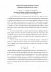As was pointed out in the introduction of this paper, thermal runaways linked to mixing Fig. 10. (a) Histogram of percentage (light grey filled), cumulative percentage of the vessel volume (dashed line) and cumulative percentage of the quenched volume (full line) versus normalised scalar concentration, at t = 7 s. (b) Time evolution of the cumulative curves for the quenched volume percentage versus the normalised scalar concentration; dashed line: minimum scalar concentration equal to 4.38 × 10−2 ; black dot: location used for an example detailed in the text. The conditions were d = 7.2 mm, V = 6 m s−1 , N = 100 RPM. J.-P. Torré et al. / Chemical Engineering Science 63 (2008) 924 – 942 937 Fig. 11. Cumulative curves of the percentage of quenched volume versus time for various jet inlet conditions. The description of each case is given in Table 2. Table 2 Jet injection parameters: jet diameter, jet velocity, jet momentum flux, jet flow rate and the corresponding curve numbers of Fig. 11 d (mm) V (m s−1 ) M (kg m s−2 ) Q (l min−1 ) Curve # (Fig. 11) 7.2 10 15 7.2 10 10 7.2 15 10 15 2 2 2 6 4.5 6 10 6 10 10 0.162 0.313 0.705 1.461 1.586 2.819 4.059 6.343 7.830 17.618 4.89 9.42 21.21 14.66 21.21 28.27 24.43 63.62 47.12 106.03 1 2 3 4 5 6 7 8 9 10 both on the application studied and on the safety level considered for the reactor quenching, and has been calculated on the basis of real industrial data. When the liquid in the jet, which is subsequently identified via the concentration of a transported scalar variable (defined to take a value of unity in the jet), is mixed in the vessel, its concentration, C, in each numerical cell is tracked with time. The concentration values are everywhere zero before injection starts, and reach the equilibrium concentration, denoted Cinf , everywhere at infinite time. However, there is a large excess of stopper so we introduce Cmin which is the minimum quantity of stopper that must be injected to quench the reaction if it is mixed uniformly throughout the vessel. The normalised stopper concentration, C ∗ , is defined as ∗ is defined as the ratio of C C/Cinf . Finally, Cmin min to Cinf and represents the normalised minimum concentration necessary to ∗ quench the reaction throughout the vessel. The value of Cmin used here is based on a real industrial system used in polymerisation reactors and equals 4.38 × 10−2 . The concentration was tracked with time in the whole vessel volume and analysis of this concentration data forms the basis of the definition of the mixing criteria presented below. The percentage of the vessel volume which falls within a given concentration range was tracked with time. An example is presented in Fig. 10(a) for a case with a jet diameter of 7.2 mm and a jet velocity equal to 6 m s−1 , at a time of 7 s after the beginning of injection. As the time increases, the spread of the histogram decreases and the data are centred on the equilibrium concentration. The exact experimental value of this final concentration Cinf was equal to 4.87 × 10−3 , calculated as the ratio of the injected volume (0.533 l) to the vessel volume (109.533 l). The value determined numerically, which is used in the subsequent calculations, was 4.94 × 10−3 , with the small difference being due to the removal of a small quantity of liquid at the free surface to keep the liquid level constant in the simulations (see Section 3). A pertinent analysis of these data was the use of the cumulative curves shown in Fig. 10(a). The curve represented with a dashed line is the classical cumulative curve obtained directly from the histogram data, and each point gives the percentage of the vessel volume with a concentration below the value given by the abscissa. The full line shows the complement of this value and represents the cumulative percentage of the quenched volume of the vessel versus the scalar concentration. Fig. 10(b) shows the evolution over time of this curve with a 0.2 s interval. For example, the black dot in Fig. 10(b), which corresponds to a time of 1.6 s after injection started, indicates that 42% of the vessel volume has a concentration above the minimum concentration required to quench the reaction, therefore, in 42% of the vessel volume the runaway reaction would be quenched. It should be noted that we assume that there are no micro-mixing limitations and that therefore once a critical concentration is reached in a computational volume the reaction is assumed to be quenched. ∗ If the percentage of quenched volume relative to Cmin is plotted versus time (the value at the intersection of the cumulative curve and the vertical dashed line of Fig. 10(b)), the new curve, which gives the percentage of the vessel volume 938 J.-P. Torré et al. / Chemical Engineering Science 63 (2008) 924 – 942 Fig. 12. Evolutions of the various mixing criteria versus jet momentum flux and jet momentum flux to the power −0.5, at N = 100 RPM; (a) t50 versus M; (b) t50 versus M −0.5 and its correlation; (a) t90 versus M; (b) t90 versus M −0.5 . quenched versus time, is named the quenching curve. This is a useful way to compare the effect of different injection conditions on the quenching efficiency. Fig. 11 shows the quenching curves for all of the injection conditions investigated numerically at N = 100 RPM, and the jet injection conditions are summarised in Table 2. It is clear that, for a constant agitator speed, the quenching efficiency is affected significantly by the jet injection conditions. The different curves of Fig. 11 correspond to the different injection conditions and each is referenced using the short-hand notation (d [mm], V [m s−1 ]). Although the cases (15 mm, 2 m s−1 ) and (10 mm, 4.5 m s−1 ) have the same jet flow rate, their quenching curves are not coincident. In addition, when the quenched volume is below 60%, it is noted that the time to quench the same volume is shorter for the (7.2 mm, 6 m s−1 ) case than the (15 mm, 2 m s−1 ) case which have flow rates equal to 14.86 and 21.21 l min−1 , respectively. Thus, the evolution of the curves cannot be explained by considering the jet flow rate alone. In contrast when the quenched volume is below 60% all of the curves in Fig. 11 shift from the right to the left as the jet momentum flux increases. Therefore, although the effect of the liquid jet density was not investigated in this study, the quenching efficiency was founded to depend on the jet momentum flux if the quenched volume is below 60% but not directly on the jet flow rate. For a quenched volume between 60% and 100%, the conclusions and the dependence on the momentum flux are not so clear. Nevertheless, the results showed an optimum jet momentum flux, based on quenching a high percentage of the vessel volume, as the cases (7.2 mm, 6 m s−1 ) and (10 mm, 4.5 m s−1 ) led to the shortest quenching time for 90% of the vessel compared with higher momentum flux cases. 7.2. Mixing criteria: t50 and t90 The times t50 and t90 , which represent the time required to quench 50% and 90% of the vessel volume, respectively, have also been determined and are used to quantify the optimum injection conditions at N = 100 RPM. The value of t50 decreases as the jet momentum flux increases, as shown in Fig. 12(a), and was found to depend linearly on the inverse of the momentum flux to the power 0.5, as shown in Fig. 12(b). A power law between t90 and M was not observed as a minimum was obtained for the cases (7.2 mm, 6 m s−1 ) and (10 mm, 4.5 m s−1 ) as shown in Fig. 12(c), whilst the optimum jet momentum flux was clearly observed as being Mopt ≈ 1.5 kg m s−2 . A higher jet momentum flux gave a constant value of t90 , as shown in Fig. 12(d), which means that, at this rotation speed, it is not necessary to increase M to Mopt to have a better quenching of 90% of the vessel volume. 8. Improving reactor quenching This section is devoted to the study of the influence of the jet trajectory on reactor quenching. As it has already been demonstrated that the injection parameters influence the jet trajectory significantly, Fig. 13 is used to show the evolution of the quenched volume with time for four different jet injection J.-P. Torré et al. / Chemical Engineering Science 63 (2008) 924 – 942 939 ∗ versus time (yellow: quenched; red: not quenched), and jet profiles at T (300 Lagrangian particles Fig. 13. Isovolumes of scalar concentration greater than Cmin inj coloured by the Lagrangian particle travel time normalised by Tinj ): (a) (7.2 mm, 2 m s−1 ), M = 0.162 kg m s−2 ; (b) (7.2 mm, 6 m s−1 ), M = 1.461 kg m s−2 ; (c) (10 mm, 4.5 m s−1 ), M = 1.586 kg m s−2 ; (d) (15 mm, 10 m s−1 ), M = 17.618 kg m s−2 . N = 100 RPM. 940 J.-P. Torré et al. / Chemical Engineering Science 63 (2008) 924 – 942 conditions. The quenched volume is represented by the iso∗ , as this represents the region where volume where C ∗ > Cmin the reaction is quenched. The conclusions obtained from this analysis of the evolution of the quenched volume versus time are affected by the fact that a full transient simulation was not made in which a SM modelled the rotation of the impeller blades, and therefore the transport by blade motion of the fluid already quenched to regions where the fluid is not quenched is not included. This is clearly a significant assumption, imposed by computational constraints but the case analysed here corresponds to the worse case scenario. As shown previously, the minimum value of t90 was characterised by an optimum jet momentum flux close to 1.5 kg m s−2 . This optimal jet momentum condition is presented in Figs. 13(b) and (c), while Figs. 13(a) and (d) show the cases where M < Mopt and M > Mopt , respectively. As shown in Fig. 13(a), the fluid injected with the weakest momentum flux leads to a jet trajectory that causes quenching of the top part of the vessel first, then the region close to the vessel axis, and finally the vessel periphery. In contrast, the highest jet momentum flux leads to the quasi-instantaneous transport of the fluid to the bottom of the tank, as shown in Fig. 13(d). Although this condition leads to the lowest value of t50 , it was not the optimal condition to quench 90% of vessel volume. The fluid, once it arrives in the bottom part of the vessel, has difficulty reaching the top part of the vessel because the mixing process is limited by the macro-mixing. In spite of the turbulence created by the high velocity jets which should enhance mixing, these conditions were not optimal for an agitator rotation speed of 100 RPM. In spite of the differences in the jet diameters and jet velocities, the cases presented in Figs. 13(b) and (c) gave rise to the lowest values of t90 and good quenching conditions were obtained for very similar jet trajectories. Figs. 13(b) and (c) show an efficient way to mix the fluid jet. The jet trajectories are such that the injected fluid is able to flow in several directions: one towards the top which transported the jet fluid into the upper part of the vessel, one laterally toward the middle of the tank allowing quenching of the central portion of the vessel and with this fluid getting mixed into the bottom of the vessel due to the agitator pumping effect, and one part towards the vessel periphery. The consequence is that the jet fluid is transported via the bulk flow to different locations and this has a really positive effect if 90% of the volume is to be quenched. This produces the same effect as having multiple feed locations, a situation which is well-known to reduce the mixing time of an additive in batch or semi-batch reactors. Therefore, it is clear that the quenching efficiency depends on the jet trajectory. As the jet trajectory has been found to depend directly on the jet momentum flux, the jet trajectory may be controlled via its momentum flux and it is not the jet with the greatest penetration (as usually suggested) but one that produced the correct penetration to maximise the benefits of the bulk flow pattern that is optimal. 9. Conclusions The fluid injection via a jet at the flat free surface of a partially baffled agitated vessel has been studied both experimentally and numerically to improve the understanding of the fluid mechanics of a model system related to the quenching of runaway reactions in batch industrial polymerisation reactors. The experiments and the simulations have been carried out using water for both the stirred and injected fluids, using various jet cross-sections, injection velocities and agitator rotation speeds. Experimentally, the jet trajectories have been visualised using UV fluorescence to limit the uncertainties associated with the entrainment of air bubbles by the free-falling jet, as the focus this study is the liquid injection. This method was shown to perform well, and allowed the liquid jet penetration behaviour into the bulk during the injection period to be visualised. It was shown that the jet trajectory depends on the jet momentum flux and its relative magnitude compared with tangential velocity of the bulk flow in the vessel which develops in the top part of this under-baffled stirred vessel. Numerically, an Eulerian–Lagrangian approach which used a single-phase flow model in which the modification of the bulk hydrodynamics by the jet momentum was taken in account has been developed to investigate the effect of the jet injection parameters on the jet trajectory. The analysis of Lagrangian particles trajectories showed very clearly in three dimensions how the jet penetrates and then mixes into the bulk. Comparison of the experimental data obtained for a single jet diameter with these CFD predictions showed very good agreement. At the same time, the transport of a passive scalar was used in order to correlate the influence of the jet trajectory with the quenching efficiency, by analysing the scalar concentration distribution versus time. By considering that in each vessel elementary volume the reaction was quenched when the scalar concentration exceeded a minimum required value, the definition of the global mixing criteria t50 and t90 (corresponding to 50 and 90% of the vessel volume quenched, respectively) was found to be useful to quantify the effect of the injection parameters on the quenching rate. At the rotation speed of 100 RPM, the jet momentum flux was found to be correlated with the jet trajectory and the analysis of the passive scalar concentration in the vessel revealed that the quenching efficiency depended on this jet trajectory. The main conclusions can be summarised as follows: (i) a low jet momentum flux lead to weak downward jet penetration. This was caused by a deflection of the jet plume very close to the free surface due to the high tangential bulk fluid movement which exists in the upper part of this under-baffled stirred vessel. The injected fluid is trapped by the central vortices and therefore does not mix efficiently in the whole vessel; (ii) a jet momentum flux of around 1.5 kg m s−2 lead to the lowest time to quench 90% of the vessel volume and this value was deemed to be the optimal jet momentum flux at N = 100 RPM. The analysis of the jet trajectories obtained in this case revealed that the injected fluid was transported optimally in the vessel by maximising the benefits of the bulk flow pattern; (iii) a high jet momentum flux lead the injected fluid to reach the bottom of the vessel very quickly, and to be poorly J.-P. Torré et al. / Chemical Engineering Science 63 (2008) 924 – 942 dispersed. As the transport of this fluid is linked to macromixing limitations, this condition was not optimal in the vessel studied, where the flow is mainly tangential in the upper vessel. These limitations would have a stronger effect if the agitator velocity is decreased. Therefore, it was demonstrated that this simplified CFD modelling provides a valuable qualitative description of the trajectory of a liquid jet, having the same physical properties as the stirred liquid, injected at the flat free surface of a partially baffled agitated vessel. The numerical method used with the global mixing criteria t50 and t90 is useful for process safety purposes in order to quantify the influence of the injection parameters on the quenching efficiency. Future work will investigate the challenging problem of the study of jet injection at higher agitator rotation speed where the effect of the free surface shape deformation cannot be neglected. The authors would like to thank the technical staff of the LGC of Toulouse and A. Muller is particularly acknowledged for his excellent technical assistance. A large part of the computer resources needed were provided by the Scientific Grouping CALMIP, and our thanks are expressed to N. Renon for enabling this to happen. We also owe great thanks to I. Touche for the considerable assistance she gave with use of the supercomputer. Tessenderlo Group and ANRT are acknowledged for financial support. Appendix A. Governing equations The continuity equation is expressed as ∇ · u = 0. (1) As the standard k. model employs the eddy-viscosity hypothesis, the momentum equation may be expressed as j(u) + ∇ · (u ⊗ u) = −∇p ′ + ∇ · [eff (∇u + (∇u)T )], (2) jt where eff is the effective viscosity defined by with turb = C k2 and C = 0.09. (3)  p′ is a modified pressure (note that gravity is not included as it is absorbed into the pressure in this single-phase flow) expressed in Eq. (4) as p ′ = p + 23 k. j() + ∇ · (u) = ∇ · jt (4) The values of k and  come directly from the transport equations for the turbulent kinetic energy and the turbulence dissipation rate, which are expressed in Eqs. 5 and 6, respectively    turb j(k) ∇k + P̃ − , + ∇ · (uk) = ∇ · lam + jt k (5) (6) with C1 , C2 , k and  being model constants that are set to the usual values of 1.44, 1.92, 1.0 and 1.3, respectively. The turbulence production due to shear is given as P̃ = turb ∇u · (∇u + (∇u)T ). (7) The transport equation for the scalar  is given as j() turb + ∇ · (u) = ∇ · [(Dlam )∇],  +D jt (8) turb where Dlam  is the kinematic diffusivity of the scalar and D is the turbulent diffusivity expressed Dturb = Acknowledgements eff = lam + turb    turb lam ∇  +   + (C1 P̃ − C2 ) k 941 turb Scturb (9) with the turbulent Schmidt number, Scturb , set to 0.9. References ANSYS-CFX 11.0, 2007. User’s guide http://www.ansys.com . Aubin, J., Kresta, S.M., Bertrand, J., Xuereb, C., Fletcher, D.F., 2006. Alternate operating methods for improving the performance of continuous stirred tank reactors. Chemical Engineering Research and Design 84 (A7), 569– 582. Balasubramanian, S.G., Louvar, J.F., 2002. Study of major accidents and lessons learned. Process Safety Progress 21 (3), 237–244. Balasubramanian, S.G., Dakshinamoorthy, D., Louvar, J.F., 2003. Shortstopping runaway reactions. Process Safety Progress 22 (4), 245–251. Bałdyga, J., Pohorecki, R., 1995. Turbulent micromixing in chemical reactors—a review. The Chemical Engineering Journal and the Biochemical Engineering Journal 58 (2), 183–195. Baldyga, J., Bourne, J.R., Yang, Y., 1993. Influence of feed pipe diameter on mesomixing in stirred tank reactors. Chemical Engineering Science 48 (19), 3383–3390. Barton, J.A., Nolan, P.F., 1989. Incidents in the chemical industry due to thermal runaway chemical reactions. In: Hazards X: Process Safety in Fine and Specialty Chemical Plants, Symposium Series, vol. 115, pp. 3–18. Bhattacharya, S., Kresta, S.M., 2006. Reactor performance with high velocity surface feed. Chemical Engineering Science 61 (9), 3033–3043. Bidone, G., 1829. Expériences sur la forme et sur la direction des veines et des courants d’eau lances par diverses ouvertures. Imprimerie Royale, Turin, 1–136. Bin, A.K., 1993. Gas entrainment by plunging liquid jets. Chemical Engineering Science 48 (21), 3585–3630. Butcher, M., Eagles, W., 2002. Fluid mixing re-engineered. Chemical Engineering 733, 28–29. Chanson, H., Aoki, S., Hoque, A., 2004. Physical modelling and similitude of air bubble entrainment at vertical circular plunging jets. Chemical Engineering Science 59 (4), 747–758. Dakshinamoorthy, D., Louvar, J.F., 2006. Hotspot distribution while shortstopping runaway reactions demonstrate the need for CFD models. Chemical Engineering Communications 193, 537–547. Dakshinamoorthy, D., Khopkar, A.R., Louvar, J.F., Ranade, V.V., 2004. CFD simulations to study shortstopping runaway reactions in a stirred vessel. Journal of Loss Prevention in the Process Industries 17, 355–364. Dakshinamoorthy, D., Khopkar, A.R., Louvar, J.F., Ranade, V.V., 2006. CFD simulation of shortstopping runaway reactions in vessels agitated with impellers and jets. Journal of Loss Prevention in the Process Industries 6, 570–581. 942 J.-P. Torré et al. / Chemical Engineering Science 63 (2008) 924 – 942 Danckwerts, P.V., 1952. The definition and measurement of some characteristics of mixtures. Applied Scientific Research A (3), 279–296. Davoust, L., Achard, J.L., El Hammoumi, M., 2002. Air entrainment by a plunging jet: the dynamical roughness concept and its estimation by a light absorption technique. International Journal of Multiphase Flow 28 (9), 1541–1564. El Hammoumi, M., Achard, J.L., Davoust, L., 2002. Measurements of air entrainment by vertical plunging liquid jets. Experiments in Fluids 31, 624–638. Etchells, J.C., 1997. Why reactions run away. Organic Process Research and Development 1, 435–437. Fowler, A.H.K., Baxter, A., 2000. Fires, explosions and related incidents at work in Great Britain in 1996/97 and 1997/98. Journal of Loss Prevention in the Process Industries 13 (6), 547–554. Fowler, A.H.K., Hazeldean, J.A., 1998. Fires, explosions and related incidents at work in Great Britain in 1994/95 and 1995/96. Journal of Loss Prevention in the Process Industries 11 (5), 347–352. Grotjans, H., Menter, F.R., 1998. Wall functions for general application CFD codes. In: ECCOMAS 98, Proceedings of the Fourth European Computational Fluid Dynamics Conference, Wiley, New York, pp. 1112–1117. Gustin, J.L., 1991. Runaway reactions, their courses and the method to establish safe process conditions. Journal de Physique III France 1, 1401–1419. Hiby, J.W., 1981. Definition and measurement of the degree of mixing in liquid mixtures. International Chemical Engineering 21 (2), 197–204. Kammel, U., Schlüter, S., Steiff, A., Weinspach, P.M., 1996. Control of runaway polymerization reactions by injection of inhibiting agents—a contribution to the safety of chemical reactors. Chemical Engineering Science 51 (10), 2253–2259. Kersten, B., Ohl, C.D., Prosperetti, A., 2003. Transient impact of a liquid column on a miscible liquid surface. Physics of Fluids 15 (3), 821–824. McCarthy, M.J., Molloy, N.A., 1974. Review of stability of liquid jets and the influence of nozzle design. Chemical Engineering Journal 7, 1–20. McIntosh, R.D., Nolan, P.F., 2001. Review of the selection and design of mitigation systems for runaway chemical reactions. Journal of Loss Prevention in the Process Industries 14 (1), 27–42. McKeogh, E.J., Ervine, D.A., 1981. Air entrainment rate and diffusion pattern of plunging liquid jets. Chemical Engineering Science 36, 1161–1172. Muppidi, S., Mahesh, K., 2005. Study of trajectories of jets in crossflow using direct numerical simulations. Journal of Fluid Mechanics 530, 81–100. Nere, N.K., Patwardhan, A.W., Joshi, J.B., 2003. Liquid-phase mixing in stirred vessels: turbulent flow regime. Industrial and Engineering Chemistry Research 42, 2661–2698. Platkowski, K., Reichert, K.H., 1999. Short stopping of runaway methyl methacrylate polymerizations. Chemical Engineering Technology 22 (12), 1035–1038. Pope, S.B., 2000. Turbulent Flows. Cambridge University Press, Cambridge, UK. Rajaratnam, N., 1976. Developments in Water Science: Turbulent Jets. Elsevier Scientific Publishing Co, New York, USA. Sallam, K.A., Dai, Z., Faeth, G.M., 2002. Liquid breakup at the surface of turbulent round liquid jets in still gases. International Journal of Multiphase Flow 28, 427–449. Savart, F., 1833. Mémoire sur la constitution des veines liquides lancées par des orifices circulaires en mince paroi. Annales de Chimie et de Physique 53, 337–386. Storr, G.J., Behnia, M., 1999. Experiments with large diameter gravity driven impacting liquid jets. Experiments in Fluids 27, 60–69. Torré, J.P., Fletcher, D.F., Lasuye, T., Xuereb, C., 2007a. An experimental and computational study of the vortex shape in a partially baffled agitated vessel. Chemical Engineering Science 62 (7), 1915–1926. Torré, J.P., Fletcher, D.F., Lasuye, T., Xuereb, C., 2007b. Transient hydrodynamics and free surface capture of an under-baffled stirred tank during stopping. Chemical Engineering Research Design 85 (A5), 626–636. Torré, J.P., Fletcher, D.F., Lasuye, T., Xuereb, C., 2007c. Single and multiphase CFD approaches for modelling partially baffled vessels: comparison of experimental data with numerical predictions. Chemical Engineering Science 62 (22), 6246–6262. Verschuren, I.L.M., Wijers, J.G., Schoenmakers, G.J.H.A., Jeurissen, F.G.H., Keurentjes, J.T.F., 2001. Determination of the mixing rate of a high velocity feed stream in agitated vessels. Chemical Engineering Communications 188, 59–79. Verschuren, I.L.M., Wijers, J.G., Keurentjes, J.T.F., 2002. Large-scale oscillations of a feedstream inside a stirred tank reactor. A.I.Ch.E. Journal 48 (9), 1888–1995. Westerterp, K.R., Molga, E., 2004. No more runaways in chemical reactors. Industrial and Engineering Chemistry Research 43, 4585–4594. Westerterp, K.R., Molga, E., 2006. Safety and runaway prevention in batch and semibatch reactors—a review. Chemical Engineering Research and Design 84 (A7), 543–552. Zaldívar, J.M., Cano, J., Alós, M.A., Sempere, J., Nomen, R., Lister, D., et al., 2003. A general criterion to define runaway limits in chemical reactors. Journal of Loss Prevention in the Process Industries 16 (3), 187–200.