Effects of Linking a Soil-Water-Balance Model with a Groundwater-Flow Model

Effects of Linking a Soil-Water-Balance Model with a Groundwater-Flow Model by Jennifer S. Stanton1 , Derek W. Ryter2 , and Steven M. Peterson2 Abstract A previously published regional groundwater-flow model in north-central Nebraska was sequentially linked with the recently developed soil-water-balance (SWB) model to analyze effects to groundwater-flow model parameters and calibration results. The linked models provided a more detailed spatial and temporal distribution of simulated recharge based on hydrologic processes, improvement of simulated groundwater-level changes and base flows at specific sites in agricultural areas, and a physically based assessment of the relative magnitude of recharge for grassland, nonirrigated cropland, and irrigated cropland areas. Root-mean-squared (RMS) differences between the simulated and estimated or measured target values for the previously published model and linked models were relatively similar and did not improve for all types of calibration targets. However, without any adjustment to the SWB-generated recharge, the RMS difference between simulated and estimated base-flow target values for the groundwater-flow model was slightly smaller than for the previously published model, possibly indicating that the volume of recharge simulated by the SWB code was closer to actual hydrogeologic conditions than the previously published model provided. Groundwater-level and base-flow hydrographs showed that temporal patterns of simulated groundwater levels and base flows were more accurate for the linked models than for the previously published model at several sites, particularly in agricultural areas. Introduction Information about recharge is critical for understanding the long-term sustainability of an aquifer. However, estimating recharge for large areas is challenging because of the many uncertainties associated with generalizing factors such as climate, soil and unsaturated-zone properties, land cover, land slope, and depth to water table that affect recharge over regional scales (Sophocleous 2004). Localscale methods such as the use of chemical tracers and matric potentials in the unsaturated zone provide more accurate information at point locations (Healy 2010) but 1 Corresponding author: U.S. Geological Survey, 5231 South 19th St., Lincoln, NE 68512, (402) 261-0458; fax: (402) 328-4101; jstanton@usgs.gov 2 U.S. Geological Survey, 5231 South 19th St., Lincoln, NE 68512. Received February 2012, accepted August 2012. Published 2012. This article is a U.S. Government work and is in the public domain in the USA. doi: 10.1111/j.1745-6584.2012.01000.x NGWA.org rarely are there more than a few local estimates available for any single region of interest. Partly, as a result of the uncertainties associated with regional recharge estimates, recharge frequently is used as a calibration parameter for groundwater-flow models (Luckey et al. 1986; Peterson 2007; Stanton et al. 2010). Fully integrated hydrologic models (Markstrom et al. 2008; Schmid and Hanson 2009; Hanson et al. 2010) have been developed to estimate recharge through coupling of groundwater and landscape processes but can be difficult to implement at regional scales. Soil-water-balance (SWB) models represent a simpler approach than fully integrated hydrologic models for estimating recharge and crop-irrigation requirements (Schroeder et al. 1994; Kendy et al. 2003; Vaccaro 2007; Kahle et al. 2011). The SWB model code has recently been developed by the U.S. Geological Survey (USGS) (Westenbroek et al. 2010) to estimate recharge using readily available public data for air temperature, precipitation, soil properties, land-surface elevation, and land use/land cover. Vol. 51, No. 4–Groundwater–July-August 2013 (pages 613–622) 613 The USGS, in collaboration with State and local natural resource-management agencies, developed a regional groundwater-flow model called the Phase-Two ElkhornLoup Model (ELM2) to characterize the groundwater system and assess the effect that historical and future groundwater pumpage (for irrigation) has on surface water in north-central Nebraska (Stanton et al. 2010). Calibration results for that model indicated that, although the model reasonably replicated hydrogeologic conditions for most of the study area, simulated groundwater levels and base flows in some agricultural areas were too low. Possible explanations for this included: (1) too much simulated irrigation pumpage; (2) too little simulated recharge or irrigation return flow; and (3) recharge zones that were too large areally. The SWB model code was linked with the ELM2 to: (1) generate a more detailed spatial and temporal representation of recharge than was used for the published ELM2; (2) provide a better understanding of recharge in the study area; and (3) improve calibration in areas where the groundwater levels and base flows were too low. A similar type of linkage has been performed using the HELP model and global climate models (Toews and Allen 2009). The purpose of this study is to analyze the effects of linking an SWB model with the ELM2 on groundwater-flow model parameters and calibration results, determine whether the linked models can improve the understanding of hydrologic processes, and assess the advantages and limitations of linking SWB and MODFLOW models. The study area covers approximately 30,000 mi2 (77,700 km2 ) in north-central Nebraska (Figure 1) (Stanton et al. 2010). The area consists of loess hills, dissected loess plains, river valleys, plains, sandy plains, broken lands verging on river valleys, wet meadows and marsh plains, and the Sand Hills (U.S. Environmental Protection Agency 2003). Row-crop agriculture typically occurs in the flat or gently sloping areas classified as river valleys or plains. In 2005, about 13% of the study area was used for irrigated agriculture, and 5% of the study area was used for nonirrigated agriculture (Center for Advanced Land Management Information Technologies 2007). The rest of the study area is primarily grassland used for grazing livestock and is not irrigated. Methods The ELM2 groundwater-flow model and SWB model were constructed independently and then sequentially linked through Parameter Estimation (PEST) software (Doherty 2008a, 2008b) to allow simultaneous adjustment of surface and subsurface properties during calibration. The two models were linked using two approaches: (1) a semicalibrated linked model (SCLM) and (2) a fully calibrated linked model (FCLM). Recharge for 1940 through 2005 and horizontal hydraulic conductivity (Kh ) results from the ELM2, SCLM, and FCLM were compared to determine the effect of linking the SWB and groundwater-flow models on those parameter values. In addition, calibration statistics from the SCLM and 614 J.S. Stanton et al. Groundwater 51, no. 4: 613–622 Figure 1. Location of the Elkhorn-Loup Model study area, Elkhorn and Loup River Basins, Nebraska. FCLM were compared with the ELM2 to evaluate whether the linked models improved the calibration of the simulation. Groundwater-Flow Model Construction The previously published ELM2 (Stanton et al. 2010) was constructed using MODFLOW-2005 (Harbaugh 2005). The ELM2 used a uniformly spaced horizontal grid of 1-mile-by-1-mile (1.6-km-by-1.6-km) cells covering an active model area of 29,707 mi2 (76,941 km2 ) and a single vertical layer with annual stress periods. The model simulated conditions from predevelopment through 2005 and was calibrated using an automated parameterestimation method to optimize the fit to pre-1940 groundwater levels and base flows, 1945 through 2005 decadal groundwater-level changes, and 1940 through 2005 annual base flows. Simulated recharge in the ELM2 model was composed of water from several sources: precipitation, additional recharge ascribed to irrigated and nonirrigated agricultural lands, and canal seepage. Spatial variation of recharge from precipitation was enabled by dividing the study area into 20 recharge zones. For the pre-1940 period, recharge from precipitation was a static value representing long-term average conditions. Temporal variation of recharge from precipitation for 1940 through 2005 was simulated by dividing each of the 20 recharge zones into 4 to 9 time periods. This created 135 recharge parameters that were independently adjusted through the calibration process. In addition, 0.5 in./year (1.3 cm/year) of recharge was added to nonirrigated cropland areas, and 1.0 in./year (2.5 cm/year) of recharge was added to irrigated cropland areas. The concept that recharge rates are smallest in natural rangeland areas, moderate in nonirrigated cropland areas, and largest in irrigated agricultural areas is similar to that reported by Sophocleous (2004) and Scanlon et al. (2005) and used in previous groundwater-flow models in Nebraska (Luckey and Cannia 2006; Peterson 2007; Carney 2008; Peterson et al. 2008). Nonirrigated cropland is associated with larger recharge than rangeland because NGWA.org of changes to soil structure, seasonal vegetation coverage, wilting point, and rooting depth (Sophocleous 2004). Irrigation further increases recharge through the addition of water to the soil profile (McMahon et al. 2006). For the ELM2, excess water due to irrigation inefficiency was not included as a separate source of recharge. Instead, pumpage for irrigation was estimated as a crop-irrigation requirement instead of total pumpage. These values represented a net irrigation pumpage that did not include excess water needed to satisfy irrigation inefficiencies. This was deemed appropriate because the aquifer was a single-unconfined system and return flow was expected to affect recharge within the same stress period. Canal seepage recharge was simulated for any grid cell coinciding with a canal, canal lateral, or land that received canal water for irrigation. The amount of canal seepage was obtained from annual canal and lateral losses calculated using measured amounts of water entering the canal, delivered to fields, and returning to streams. SWB Model Construction The SWB model calculates the portions of precipitation, snowmelt, and applied irrigation water that become surface runoff, evapotranspiration (ET), and recharge using a modified Thornthwaite-Mather soil-water accounting method to track the soil water in each grid cell with time (Thornthwaite and Mather 1957; Westenbroek et al. 2010). Recharge, represented in the SWB model by deep percolation, that is, potential recharge, is the surplus water in the root zone of the soil column. Surplus water is calculated by subtracting the sum of the outputs (ET, surface runoff, plant interception) from the inputs (precipitation, snowmelt, irrigation water, surface runoff from adjacent cells). Parameters that control flow and loss of water on the ground surface and within the soil include the soil available water capacity (AWC), hydrologic soil group (Musgrave 1955), land use/land cover, and direction of surface-water runoff. Surface-water runoff is calculated using the Natural Resources Conservation Service (NRCS) curve-number method of Cronshey et al. (1986) and is affected by soil properties and moisture content. Precipitation that falls as snow is stored on the surface until temperature causes it to melt (Westenbroek et al. 2010). The direction of surface flow is determined from land-surface elevations and is used to route surface runoff to adjacent cells. Runoff that is transferred between cells is tracked as inflow and outflow. If runoff water is routed to a closed surface depression, available water can exceed ET and soil-moisture demands. In these cases, the SWB code does not carry extra water that is not allowed to infiltrate over to the following day. This is tracked as rejected recharge. Infiltration and runoff also are affected by frozen ground, which is tracked using a continuous frozen-ground index (Molnau and Bissell 1983). There are several methods available in the SWB code to estimate ET, but for this study the Hargreaves and Samani’s (1985) method was used, which uses the daily high and low air temperatures to calculate potential ET. NGWA.org The original SWB code was modified to include effects of crop water use on ET and the addition of irrigation water to satisfy crop water-use requirements in irrigated areas (Stanton et al. 2011). The volume of water necessary to maintain soil moisture in irrigated areas is assumed to be the volume of water entering the soil profile from irrigation and is calculated as the crop demand beyond available infiltrated precipitation. Irrigation efficiency, the source of irrigation water, and the availability of shallow groundwater to satisfy crop water demands are not defined in the model formulation. The MODFLOW Farm Process extension (MF-FMP; Schmid and Hanson 2009) offers a more comprehensive approach for estimating effects of irrigation on the groundwater-flow system. However, for this study, irrigation demand simulated by SWB was not used to represent irrigation pumpage in the groundwater-flow model, and recharge associated with irrigation inefficiency was already included in the net irrigation pumpage values; therefore, these were not important limitations. The SWB model was constructed on a horizontal grid identical to that used by the groundwater-flow model to simulate daily recharge from 1939 through 2005. Each model cell was attributed with land cover, soil properties, direction of surface flow, and daily climate data. The land-cover category was defined for each 1mile (1.6-km) model grid cell as the dominant land use within that cell, as mapped in the 30-m resolution 2001 National Land Cover Database (Multi-Resolution Land Characteristics Consortium 2001). Soil properties were derived from the U.S. General Soil Map (STATSGO2) (U.S. Department of Agriculture 2006). 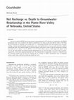Root-zone depths were assigned based on hydrologic soil group (Figure 2) and land-cover classification because the same vegetation will send roots to different depths for different soil types (Thornthwaite and Mather 1957; Westenbroek et al. 2010). Surface-water flow directions were derived from digital elevation models (U.S. Geological Survey and Nebraska Department of Natural Resources 1998). To represent climatic conditions, daily precipitation and temperature data for 1939 through 2005 were interpolated from weather data compiled from the National Climatic Data Center (2010). Precipitation values were interpolated using an inverse-distance weighted method (power = 2, variable search radius of 12 points; Johnston et al. 2001), and temperature values were interpolated using a Kriging method (spherical semivariogram model, variable search radius of 12 points; Johnston et al. 2001). Excessive recharge was limited by assigning a maximum recharge rate of 2, 0.6, 0.24, and 0.12 in/d (5, 1.5, 0.61, and 0.30 cm/d) for hydrologic soil group A, B, C, and D, respectively. Soil moisture in irrigated agricultural areas was maintained above 50% of the soil AWC during the growing season. Construction of Sequentially Linked Models The SCLM was used to determine whether SWBgenerated recharge for 1940 through 2005 was comparable to ELM2-calibrated recharge and whether model J.S. Stanton et al. Groundwater 51, no. 4: 613–622 615 Figure 2. Hydrologic soil groups, Elkhorn and Loup River Basins, Nebraska (Source: U.S. Department of Agriculture 2004). performance improved by using unadjusted SWB model inputs. For the SCLM, the SWB model was processed using best estimates of initial SWB model inputs to obtain daily recharge upscaled to annual stress periods by totaling daily recharge on an annual basis and then converting to an average rate for each model cell. Canal seepage, as estimated for the ELM2, was then added to the SWB-generated recharge, and the ELM2 simulation was reprocessed using the updated combined recharge. Thus, uncalibrated recharge from the SWB model was used to replace the previously calibrated recharge values from the ELM2. The SCLM did not include additional recharge on nonirrigated and irrigated cropland. All other model inputs from the ELM2, including long-term average recharge for the pre-1940 period, remained the same (Stanton et al. 2010). The FCLM was processed through the PEST software (Doherty 2008a, 2008b) to allow surface and subsurface properties to adjust simultaneously during calibration. The calibration approach included the following processing sequence: (1) SWB simulation to obtain daily recharge (upscaled to annual values) for each model cell; (2) add canal seepage to the SWB-generated recharge; (3) reformat the combined SWB and canal seepage recharge values as a MODFLOW recharge package file; (4) MODFLOW simulation; (5) compare simulation results with calibration targets; and (6) adjust calibration parameters. Calibration parameters included rootzone depth and NRCS runoff curve numbers in the SWB model, and horizontal hydraulic conductivity (Kh ) in MODFLOW. This sequence was repeated until the difference between simulated results and calibration target values as determined in step 5 ceased to diminish between PEST runs. Initial parameter values for the FCLM were the same as for the SCLM. Upper and lower limits were assigned to calibrated parameters to prevent extreme parameter 616 J.S. Stanton et al. Groundwater 51, no. 4: 613–622 values during calibration. Ranges of allowable NRCS runoff curve-number values were based on Cronshey et al. (1986) (Table S1). The range of allowable values for rootzone depths during calibration were calculated as ±50% of the initial values. Minimum and maximum Kh values allowed for each Kh zone during calibration were set to the same values used for the ELM2 (a lower limit of 5 feet [1.5 m] per day and an upper limit of 1000 feet [305 m] per day). A Tikhonov-regularization process (Hunt et al. 2007; Fienen et al. 2009) was used during calibration to minimize large deviations from initial Kh parameter values. The calibration targets used to determine the performance of the FCLM and adjust SWB and MODFLOW input parameters were the same as for the ELM2 (Stanton et al. 2010). That is, 506 groundwater levels (measured at 506 wells) and 20 base-flow targets (estimated at 20 streamflow-gaging stations) were used for the pre-1940 calibration period, and 3259 decadal groundwater-level changes (measured at 1454 wells) and 1435 annual baseflow targets (estimated from 38 streamflow-gaging stations and 165 low-flow measurements) were used for the 1940 through 2005 calibration period. Results and Discussion Phase-Two Elkhorn-Loup Model The spatial variation of average annual recharge rates (sum of all sources of recharge) for 1940 through 2005 as calibrated for the ELM2 (Figure 3A) (Stanton et al. 2010) was consistent with regional soil textures in the study area; rates were larger in the Sand Hills (mostly hydrologic soil group A) and smaller in the dissected Loess Plains (mostly hydrologic soil group B) but local variations due to precipitation gradients, soil characteristics, and land use/land cover were not included. The average calibrated Kh values ranged from 5.5 to 107 ft/d (1.7 to 32.6 m/d) (Figure 4A) and generally were similar to values indirectly derived using sediment grain-size analysis of samples from test holes in the study area (Conservation and Survey Division 2005; Vollertsen 2005). Overall, the ELM2 calibration process yielded simulated results that reasonably replicated calibration target values; the root-mean-squared (RMS) difference was 35.1 feet (10.7 m) for pre-1940 groundwater-level targets, 5.1 feet (1.6 m) for decadal groundwater-level changes during 1945 to 2005, and 106 cubic feet (3.00 cubic meters) per second for 1940 to 2005 annual base flows (Table 1). The RMS difference for pre-1940 groundwaterlevel target values was a small percentage (1.4%) of the total variation in simulated groundwater levels within the study area. The mean absolute difference between simulated and measured decadal groundwater-level changes (3.6 feet, or 1.1 m) was generally within the expected uncertainty of the groundwater-level-change target values (about 5 feet, or 1.5 m) (Stanton et al. 2010). The RMS difference of all simulated annual base flows was less than the averaged ranges of annual base flow at each NGWA.org A Table 1 Statistical Summary of Calibration Results Statistic B C Figure 3. Recharge assigned to (A) the calibrated PhaseTwo Elkhorn-Loup Model (Stanton et al. 2010), (B) the semicalibrated linked model (SCLM), and (C) the fully calibrated linked model (FCLM), north-central Nebraska, 1940 to 2005. of the 38 streamflow-gaging station’s respective period of record (about 160 cubic feet per second, or 4.53 cubic meters per second) (Stanton et al. 2010). However, the ELM2 was biased in some areas during the 1940 through 2005 calibration period (Figures S1 to S3). One area where simulated groundwater-level declines were greater than measured declines was north of the Elkhorn River (site W1). There, simulated declines NGWA.org Calibrated ELM2 SCLM FCLM Pre-1940 groundwater levels (506 target values), feet Mean difference 3.7 3.7 1.1 Mean-absolute 19.9 19.9 22.7ab difference Root-mean-squared 35.1 35.1 38.6 difference 1945 to 2005 decadal groundwater-level changes (weightedaverage of six 10-year time periods) (3259 target values), feet −2.0a −1.2b Mean difference −1.2b Mean-absolute 3.6 3.6 3.2ab difference Root-mean-squared 5.1 5.2 4.7 difference 1940 to 2005 base flows (1600 target values), cfs Mean difference −11b 18a −5ab Mean-absolute 53b 61a 58b difference Root-mean-squared 106 101 110 difference Notes: cfs, cubic feet per second. a Differences are significantly different than the ELM2 (Wilcoxon signed-rank test; 95% significance level) (Wilcoxon 1945). b Differences are significantly different than the SCLM (Wilcoxon signed-rank test; 95% significance level). were particularly large from 1960 to 1980. Simulated groundwater-level declines were also larger than measured declines in some areas south of the Loup River (site W10). Simulated base flow in Beaver Creek (site G6) began to decline in the 1970s whereas estimated base flow increased until about 1995. Estimated and simulated base flows declined at about the same rate from 1995 to 2005. As a result, simulated base flow of Beaver Creek was too low at the end of the calibration period. Similar patterns were observed for Cedar River (site G8) and Elkhorn River (site G2). These areas have more irrigated cropland than other parts of the study area. In addition, the temporal variability of base-flow estimates was not replicated by the simulation. Semicalibrated Linked Model For the SCLM, 1940 through 2005 recharge from the calibrated ELM2 was replaced with recharge simulated by the SWB model plus canal seepage. By using cellby-cell climate conditions, soil properties, and land use/land cover, the SCLM had a more detailed spatial distribution of recharge than the ELM2 (Figure 3B). For 2005, average recharge rates from the SCLM were 2.4 inch (6.1 cm) for grasslands, 4.4 inch (11.2 cm) for nonirrigated cropland, and 6.6 inch (16.8 cm) for irrigated cropland. These values are consistent with the conceptual model that recharge is smallest on grasslands, larger for nonirrigated cropland, and largest for irrigated cropland. J.S. Stanton et al. Groundwater 51, no. 4: 613–622 617 A B Figure 4. Horizontal hydraulic conductivity values assigned to (A) the calibrated Phase-Two Elkhorn-Loup Model (Stanton et al. 2010) and the semicalibrated linked model (SCLM), and (B) the fully calibrated linked model (FCLM), north-central Nebraska. Spatial patterns of simulated recharge not only remained larger in the Sand Hills and smaller in the dissected Loess Plains but also appear to reflect annual variation of precipitation and precipitation gradients (particularly across the Sand Hills) and more localized land use/land cover and soil characteristics. The average annual volume of simulated recharge for 1940 through 2005 was about 14% less than for the ELM2. The combination of large recharge zones and the predominant occurrence of groundwater-level measurements as targets in irrigated areas may have caused overestimation of recharge in the ELM2 because recharge is expected to be larger in irrigated areas, and to fit simulated groundwater levels to groundwater-level measurements in irrigated areas, recharge had to be increased over the entire zone. This could have caused artificially larger recharge rates. With no further adjustment to model inputs, the SCLM RMS difference was the same for pre-1940 groundwater levels, 2% larger for 1945 through 2005 decadal groundwaterlevel changes, and 5% smaller for 1940 through 2005 base flows (Table 1). Absolute differences between measured and simulated base flows were significantly larger than the ELM2 at the 95% significance level (Table 1). The selected groundwater-level hydrographs across the study area provided evidence that the SCLM yielded better replication of the temporal patterns of groundwater levels at a majority of the sites (Figures S1 and S2). The largest improvements were observed at sites in agricultural areas (W1, W6, W8, and W10). The mean absolute difference between measured and simulated groundwaterlevel changes at sites W1 and W10 (sites where simulated water levels were too low in the ELM2) was reduced by 22%. However, replication of the temporal pattern was inferior to the ELM2 at several sites (notably sites 618 J.S. Stanton et al. Groundwater 51, no. 4: 613–622 W4 and W7), and the relative magnitude of simulated groundwater-level elevations at several sites (sites W5, W7, W8, and W9) also did not improve. Comparison of SCLM with ELM2 base-flow hydrographs showed that the SCLM provided better temporal variation of simulated base flow for 8 of the 10 sites shown in Figure S3 (sites G3 and G4 did not improve), reflecting the effect of annual precipitation variation. Important improvements also were noted at several sites located downstream of irrigated areas (sites G2, G6, and G8) from about 1975 to 1995, a time when the ELM2-simulated base flows steadily declined but estimated base flows generally increased. However, the mean absolute difference between estimated and simulated base flows at site G6 (a site where simulated base flow was too low) increased by 34%. Fully Calibrated Linked Model NRCS curve number, root-zone depth, and Kh were adjusted during the calibration process of the FCLM. Optimized curve numbers and root-zone depths are listed in Table S1. Many of the calibrated curve-number values were set at the minimum value allowed during calibration, causing less simulated runoff and greater simulated recharge. In irrigated areas, smaller calibrated curve numbers could be caused by estimated net irrigation pumpage rates (a noncalibrated model parameter) that were too large. For other areas, relative sensitivity values from PEST were generally less than 5% of the largest relative sensitivity values, indicating that the model was insensitive to changes in those curve-number values and, therefore, had little effect on calibration results. In addition, Stanton et al. (2011) reported that changes to curve-number values of up to 20% yielded almost no change to simulated recharge in the High Plains. These NGWA.org results are likely related to the simple treatment of runoff by the SWB code. The SWB code handles runoff by routing it to the next down-gradient model grid cell, as determined from land-surface elevations, giving the routed water the opportunity to infiltrate in adjacent model grid cells. Therefore, changes to curve-number values only shift recharge to adjacent cells and have little effect on regional model results. The average annual simulated recharge for 1940 through 2005 from the FCLM was larger than from the SCLM and about 2% less than the ELM2-simulated average. The spatial distribution of recharge was similar to the SCLM but larger values are evident in many areas (Figure 3C). For 2005, average recharge rates from the FCLM were 2.9 inch (7.4 cm) for grasslands, 2.9 inch (7.4 cm) for nonirrigated cropland, and 6.7 inch (17.0 cm) for irrigated cropland. Recharge for grasslands and irrigated cropland were about the same as for the SCLM, whereas recharge for nonirrigated cropland was reduced by 34% and equal to recharge for grasslands. This finding provides evidence that the conceptual model (recharge for nonirrigated cropland is larger than for grassland) may need to be revised for the previously published model. The median absolute difference between the Kh values from the ELM2 and the FCLM simulations was 2.6 ft/d (0.79 m/d). The spatial distribution of Kh (Figure 4B) was mostly similar to the ELM2 and SCLM but generally larger in the southern and eastern parts of the study area, possibly reflecting the mostly coarser sediments identified from test holes in those areas. The FCLM had an RMS difference from calibration target values that was 10% larger than corresponding ELM2 results for predevelopment groundwater levels, 8% smaller for 1945 through 2005 decadal groundwater-level changes, and 4% larger for 1940 through 2005 base flows (Table 1). Differences between measured and simulated drawdowns were significantly different than the SCLM but not the ELM2 at the 95% significance level. Differences between measured and simulated base flows were significantly different than the SCLM and the ELM2 at the 95% significance level (Table 1). FCLM-simulated hydrographs of groundwater levels and base flows were closer to measured hydrographs than those from the SCLM. Although the temporal patterns at the selected well sites were simulated by the FCLM similarly as those from the SCLM, the relative magnitudes of the FCLM-simulated groundwaterlevel elevations were more similar to measured values (Figures S1 and S2). Similarly, the relative magnitudes of FCLM-simulated base flows at the selected streamflowgaging stations better matched the time series of estimated base flows than did those from the SCLM (Figures S1 and S3). The mean absolute difference between measured and simulated groundwater-level changes at sites W1 and W10 (sites where simulated water levels were too low in the ELM2) was reduced by 33% from ELM2 values. The mean absolute difference between estimated and simulated base flows at site G6 (a site where simulated base flow was too low) was reduced by 44% from ELM2 values. NGWA.org Advantages and Limitations of the Approach Linking the SWB recharge model with a numeric MODFLOW groundwater-flow model increases the quality of the model by incorporating landscape processes and characteristics to estimate and constrain the rates and spatial distribution of recharge. The landscape processes simulated by SWB include high-frequency climatic signals such as daily precipitation and soil moisture, which are a higher temporal resolution than the groundwaterflow model. These signals are not typically resolved by other processes such as MF-FMP (Schmid and Hanson 2009). By including climate signals and land use in the recharge estimation, future scenarios can be predicted in which these parameters change. Additional observations such as measured recharge and pumpage can also be used as part of the automated calibration, but reliable measurements of those types of observations were not available for this study. For this study, the SWB model provided physically based estimates of amounts of recharge for different land categories such as nonirrigated cropland and irrigated cropland, removing the need to add arbitrary amounts of recharge for those areas. As with all hydrologic models, the SWB model is a simplification of the hydrologic system and, therefore, has limitations: Daily precipitation and temperature data were distributed between weather stations using a simple interpolation method. Simulated recharge from the SWB model is highly sensitive to changes in precipitation (Stanton et al. 2011). Therefore, better methods for defining daily climate data or adjustment of interpolated precipitation values within the expected range of uncertainty between weather stations through the calibration process could improve calibration results. • The SWB model code is currently formulated such that each model cell is assigned the dominant land use/land cover within that model cell; therefore, certain landuse classifications could be either overrepresented or underrepresented in the model. • The NRCS curve-number method used by the SWB model was designed to evaluate runoff during flood events and may not accurately estimate runoff for average rainfall events (Garen and Moore 2005). In addition, runoff from a cell is assumed to infiltrate in nearby cells, shifting recharge rather than simulating overland flow to surface water storage. This is likely to cause overestimation of recharge. • For purposes of simulating irrigation water as a source of water to the soil, the current version of the SWB code tracks the mean depletion of soil moisture for each combination of land cover and hydrologic soil group. If the mean depletion percentage of soil moisture for all cells of a land-use/soil-group category is greater than the maximum allowable depletion defined by the modeler, a uniform amount of water is added to all grid cells sharing that same land-use/soil group combination. Because of variability in soil profiles and characteristic parameters within hydrologic soil groups, • J.S. Stanton et al. Groundwater 51, no. 4: 613–622 619 some cells will thus receive water in excess of field capacity, whereas others do not receive enough water to completely erase the soil-moisture deficit. • SWB as formulated for this study assigned all irrigated crops the same growing-season profile of crop wateruse coefficients, regardless of crop type or location. The SWB model could better represent the timing and amount of irrigation applications if irrigated crops were assigned crop-coefficient values specific to crop type. • Neither the SWB nor the MODFLOW models represent unsaturated zone properties or processes beneath the root zone, and potential recharge simulated by the SWB model is assumed to immediately reach the water table as recharge in the MODFLOW simulation component of the linked models used for this study. • Unlike codes such as MF-FMP (Schmid and Hanson 2009) that fully integrate the hydrologic system, SWB does not fully couple landscape, surface water, and groundwater to allow feedback between components of the hydrologic system during the simulation. General Conclusions The linked models provided a more detailed spatial and temporal distribution of simulated recharge (1940 to 2005) and better reflected precipitation gradients, land use/land cover, and localized soil properties than the ELM2. Although the ELM2 provided reasonable calibration results, the large recharge zones in that model were not based on hydrologic processes that affect recharge, but were based solely on model calibration results. By contrast, the SWB model used physically constrained parameters to calculate recharge for the linked models and a more robust assessment of the relative magnitudes of recharge for grasslands, nonirrigated croplands, and irrigated croplands in the study area. Although there were some differences between Kh values as simulated by the FCLM and ELM2, those differences were generally small and values from both models were within acceptable ranges as determined from sediment grain-size analysis of samples from test holes in the study area (Conservation and Survey Division 2005; Vollertsen 2005). Because RMS differences of simulation results from calibration target values were relatively similar and did not improve consistently for all types of calibration targets, there was not conclusive evidence from comparing RMS differences that the SCLM was a more accurate simulation than the ELM2 or that the FCLM was a more accurate simulation than the SCLM. This may be caused in part by only adjusting root-zone depth and NRCS runoff curve numbers during calibration. Previous work by Stanton et al. (2011) in the High Plains showed that recharge simulated by the SWB model was more than twice more sensitive to changes in precipitation values than to changes in root-zone depth or NRCS runoff curve number. That study also showed that differences in interpolated precipitation values from different sources yielded large enough variation to affect average simulated recharge amounts by almost 20%. Given the relatively high 620 J.S. Stanton et al. Groundwater 51, no. 4: 613–622 uncertainty of interpolated precipitation values between weather stations, it would be reasonable to introduce interpolated precipitation values in the form of pilot points (Doherty 2003) as a set of adjustable parameters. It is likely that the introduction of precipitation parameters would improve calibration results of the FCLM. Without any adjustment to the linked-model inputs, the RMS difference of the SCLM for base flows was slightly smaller than that of the ELM2, indicating that the volume of recharge simulated by the SCLM generally was closer to amounts of actual recharge in the study area. This is an important finding because recharge is one of the most difficult groundwater-budget components to quantify, and initial recharge estimates often are adjusted substantially through the calibration process to obtain simulated base flows that are consistent with estimated base flows. Visual inspection of selected groundwater-level and base-flow hydrographs showed that temporal patterns of simulated groundwater levels and base flows were more accurate for the SCLM than for the ELM2 at several sites where simulated groundwater levels and base flows were too low, indicating that the SWB model provided recharge rates that better represented actual conditions in those areas. Through calibration of the linked model, the relative magnitudes of simulated groundwater levels and base flows were further improved at many of the selected sites, but the RMS differences did not show clear improvement overall. However, the FCLM provided clear improvement at specific sites in agricultural areas noted as having poorly simulated groundwater levels and base flows in the ELM2. Acknowledgments This work was jointly funded by the Nebraska Natural Resources Commission, local Natural Resources Districts (Lower Loup, Upper Elkhorn, Lower Elkhorn, Lower Platte North, and Middle Niobrara), and the USGS. The authors would like to thank Steve Westenbroek for his help with the soil-water-balance modeling and Tom Mack, Ron Zelt, and anonymous reviewers for providing suggestions that improved the manuscript. Supporting Information Additional Supporting Information may be found in the online version of this article: Table S1. Runoff curve numbers and root-zone depths assigned to the soil-water-balance (SWB) model. Figure S1. Location of selected wells and stream flow-gaging stations used to compare performance of the Phase-Two Elkhorn-Loup Model, the semi-calibrated linked model (SCLM), and the fully calibrated linkedmodel (FCLM), north-central Nebraska. Figure S2. Measured and simulated groundwater levels, 1940 through 2005, north-central Nebraska. Figure S3. Estimated and simulated annual base flow, 1940 through 2005, north-central Nebraska. NGWA.org References Carney, C.P. 2008. Groundwater Flow Model of the Central Model Unit of the Nebraska Cooperative Hydrology Study (COHYST) Area. Lincoln, Nebraska: Cooperative Hydrology Study Sponsors. http://cohyst.dnr.ne.gov/CMU_GFMR _081224.pdf (accessed November 19, 2010). Center for Advanced Land Management Information Technologies. 2007. 2005 Nebraska Land Use Patterns. Lincoln, Nebraska: Center for Advanced Land Management Information Technologies. Remote-sensing image. http://www.calmit.unl.edu/2005landuse/statewide. shtml (accessed October 1, 2007). Conservation and Survey Division. 2005. Transmissivity of the Principal Aquifer 2005. Lincoln, Nebraska: University of Nebraska Institute of Agriculture and Natural Resources, digital data. http://snr.unl.edu/data/geographygis/NebrGIS water.asp (accessed September 16, 2012). Cronshey, R.G., R.H. McCuen, N. Miller, W. Rawls, S. Robbins, and D. Woodward. 1986. Urban Hydrology for Small Watersheds—TR-55, 2nd ed. Washington, DC: U.S. Department of Agriculture, Soil Conservation Service, Engineering Division Technical Release 55. Doherty, J. 2008a. PEST, Model Independent Parameter Estimation User Manual, 5th ed. Brisbane, Australia: Watermark Numerical Computing. http://pesthomepage.org/ (accessed October 2, 2008). Doherty, J. 2008b. PEST, Model Independent Parameter Estimation–Addendum to User Manual, 5th ed. Brisbane, Australia: Watermark Numerical Computing. http://pesthome page.org/ (accessed October 2, 2008). Doherty, J. 2003. Ground water model calibration using pilot points and regularization. Ground Water 41, no. 2: 170–177. Fienen, M.N., C.T. Muffels, and R.J. Hunt. 2009. On constraining pilot point calibration with regularization in PEST. Ground Water 47, no. 6: 835–844. Garen, D.C., and D.S. Moore. 2005. Curve number hydrology in water quality modeling—Uses, abuses, and future directions. Journal of the American Water Resources Association 41, no. 2: 377–388. Hanson, R.T., W. Schmid, C.C. Faunt, and B. Lockwood. 2010. Simulation and analysis of conjunctive use with MODFLOW’s Farm Process. Ground Water 48, no. 5: 674–689. Harbaugh, A.W. 2005. MODFLOW-2005, the U.S. Geological Survey modular ground-water model—The Ground-Water Flow Process. U.S. Geological Survey Techniques and Methods 6-A16. Reston, Virginia: USGS. Hargreaves, G.H., and Z.A. Samani. 1985. Reference crop evapotranspiration from temperature. Applied Engineering in Agriculture 1, no. 2: 96–99. Healy, R.W. 2010. Estimating Groundwater Recharge,1st ed. Cambridge, UK: Cambridge University Press. Hunt, R.J., J. Doherty, and M.J.Tonkin. 2007. Are models too simple? Arguments for increased parameterization. Ground Water 45, no. 3: 254–262. Johnston, K., J.M. Ver Hoef, K. Krivoruchko, and N. Lucas. 2001. Using ArcGIS Geostatistical Analyst. Redlands, California: ESRI ArcGIS Manual. Kahle, S.C., D.S. Morgan, W.B. Welch, D.M. Ely, S.R. Hinkle, J.J. Vaccaro, and L.L. Orzol. 2011. Hydrogeologic framework and hydrologic budget components of the Columbia Plateau Regional Aquifer System, Washington, Oregon, and Idaho. U.S. Geological Survey Scientific Investigations Report 2011–5124. Reston, Virginia: USGS. Kendy, E., P. Gerard-Marchant, M.T. Walter, Y. Zhang, C. Liu, and T.S. Steenhuis. 2003. A soil-water-balance approach to quantify groundwater recharge from irrigated cropland in the North China Plain. Hydrological Processes 17, no. 10: 2011–2031. NGWA.org Luckey, R.R. and J.C. Cannia. 2006. Groundwater Flow Model of the Western Model Unit of the Nebraska Cooperative Hydrology Study (COHYST) Area. Lincoln, Nebraska: Cooperative Hydrology Study Sponsors. http://cohyst.dnr. ne.gov/adobe/dc012WMU_GFMR_060519.pdf (accessed November 19, 2010). Luckey, R.R., E.D. Gutentag, F.J. Heimes, and J.B. Weeks. 1986. Digital simulation of ground-water flow in the High Plains aquifer in parts of Colorado, Kansas, Nebraska, New Mexico, Oklahoma, South Dakota, Texas, and Wyoming. U.S. Geological Survey Professional Paper 1400–D. Reston, Virginia: USGS. Markstrom, S.L, R.G. Niswonger, R.S. Regan, D.E. Prudic, and P.M. Barlow. 2008. GSFLOW-Coupled Ground-water and Surface-water FLOW model based on the integration of the Precipitation-Runoff Modeling System (PRMS) and the Modular Ground-Water Flow Model (MODFLOW-2005). U.S. Geological Survey Techniques and Methods 6–D1. Reston, Virginia: USGS. McMahon, P.B., K.F. Dennehy, B.W. Bruce, J.K. Böhlke, R.L. Michel, J.J. Gurdak, and D.B. Hurlbut. 2006. Storage and transit time of chemicals in thick unsaturated zones under rangeland and irrigated cropland, High Plains, United States. Water Resources Research 42: W03413. Molnau, M., and V.C. Bissell. 1983. A Continuous Frozen Ground Index for Flood Forecasting. Vancouver, Washington: 1983 Western Snow Conference Proceedings, 109–119. Multi-Resolution Land Characteristics Consortium. 2001. National Land Cover Database. U.S. Geological Survey digital data. http://www.mrlc.gov/nlcd01_data.php (accessed August 22, 2011). Musgrave, G.W. 1955. How much of the rain enters the soil? Water: U.S. Department of Agriculture. Yearbook, Washington, DC, 151–159. National Climatic Data Center. 2010. Locate weather observation station record. Asheville, North Carolina: National Climatic Data Center Web Climate Services station locator. http://www.ncdc.noaa.gov/oa/climate/stationlocator.html (accessed June 15, 2010). Peterson, S.M., J.S. Stanton, A.T. Saunders, and J.R. Bradley. 2008. Simulation of ground-water flow and effects of ground-water irrigation on base flow in the Elkhorn and Loup River Basins, Nebraska. U.S. Geological Survey Scientific Investigations Report 2008-5143. Reston, Virginia: USGS. Peterson, S.M. 2007. Groundwater Flow Model of the Eastern Model Unit of the Nebraska Cooperative Hydrology Study (COHYST) Area. Lincoln, Nebraska: Cooperative Hydrology Study Sponsors. http://cohyst.dnr.ne.gov/adobe/dc012 EMU_GFMR_090507.pdf (accessed November 19, 2010). Scanlon, B.R., R.C. Reedy, D.A. Stonestrom, D.E. Prudic, and K.F. Dennehy. 2005. Impact of land use and land cover change on groundwater recharge and quality in the southwestern U.S. Global Change Biology 11: 1577–1593. Schmid, W., and R.T. Hanson. 2009. The Farm Process Version 2 (FMP2) for MODFLOW-2005—Modifications and Upgrades to FMP1. U.S. Geological Survey Techniques in Water Resources Investigations, Book 6 : Ch. A32. Schroeder, P.R., T.S. Dozier, P.A. Zappi, B.M. McEnroe, J.W. Sjostrom, and R.L., Peyton. 1994. The hydrologic evaluation of landfill performance (HELP) model—Engineering documentation for version 3. Washington, DC: U.S. Environmental Protection Agency Office of Research and Development, EPA/600/R–94/168b. Sophocleous, M.A. 2004. Ground-water recharge and water budgets of the Kansas High Plains and related aquifers. Kansas Geological Survey Bulletin 249. Stanton, J.S., S.L. Qi, D.W. Ryter, S.E. Falk, N.A. Houston, S.M. Peterson, S.M. Westenbroek, and S.C. Christenson. 2011. Selected approaches to estimate water-budget components J.S. Stanton et al. Groundwater 51, no. 4: 613–622 621 of the High Plains, 1940 through 1949 and 2000 through 2009. U.S. Geological Survey Scientific Investigations Report 2011-5183. Reston, Virginia: USGS. Stanton, J.S., S.M. Peterson, and M.N. Fienen. 2010. Simulation of groundwater flow and effects of groundwater irrigation on stream base flow in the Elkhorn and Loup River Basins, Nebraska, 1895–2055—Phase two. U.S. Geological Survey Scientific Investigations Report 2010-5149. Reston, Virginia: USGS. Thornthwaite, C.W., and J.R. Mather. 1957. Instructions and tables for computing potential evapotranspiration and the water balance. Drexel Institute of Technology (Philadelphia) Publications in Climatology 10, no. 3: 185–311. Toews, M.W., and D.M. Allen. 2009. Evaluating different GCMs for predicting spatial recharge in an irrigated arid region. Journal of Hydrology 374, no. 3–4: 265–281. U.S. Department of Agriculture. 2006. United States General Soil Map (STATSGO2). Washington, DC: Natural Resources Conservation Service digital data. http://www.soils.usda. gov/survey/geography/statsgo/ (accessed October 13, 2009). U.S. Department of Agriculture. 2004. Hydrology: USDA-NRCS National Engineering Handbook, Part 630, Chapter 9. Washington, DC: U.S. Department of Agriculture. U.S. Environmental Protection Agency. 2003. Level III and IV Ecoregions of the Continental United States. Corvallis, 622 J.S. Stanton et al. Groundwater 51, no. 4: 613–622 Oregon: U.S. EPA Office of Research and Development—National Health and Environmental Effects Research Laboratory. http://www.epa.gov/wed/pages/ecore gions.htm (accessed November 28, 2007). U.S. Geological Survey and Nebraska Department of Natural Resources. 1998. 7.5 Minute digital elevation models—DEM-10 meter—Index for the State of Nebraska. Lincoln, Nebraska: Nebraska Department of Natural Resources geospatial data. ftp://dnrftp.dnr.ne.gov/pub/data/ dems/dem10 (accessed May 2010). Vaccaro, J.J. 2007. A deep percolation model for estimating ground-water recharge: Documentation of modules for the modular modeling system of the U.S. Geological Survey. U.S. Geological Survey Scientific Investigations Report 2006–5318. Reston, Virginia: USGS. Vollertsen, R. 2005. Nebraska Department of Natural Resources, written communication. Westenbroek, S.M., V.A. Kelson, W.R. Dripps, R.J. Hunt, and K.R. Bradbury. 2010. SWB— A modified ThornthwaiteMather Soil-Water-Balance code for estimating groundwater recharge. U.S. Geological Survey Techniques and Methods 6-A31. Reston, Virginia: USGS. Wilcoxon, F. 1945. Individual comparisons by ranking methods. Biometrics 1: 80–83. NGWA.org