JOURNAL OF GEOPHYSICAL RESEARCH, VOL. 105, NO. C10, PAGES 23,967-23,981, OCTOBER 15, 2000 Cyclone surface pressure fields and frontogenesis from NASA scatterometer (NSCAT) winds David F. Zierden, Mark A. Bourassa, and James J. O'Brien Center for Ocean-Atmospheric PredictionStudies,Florida State University,Tallahassee,32306-2840 Abstract. Two extratropicalmarine cyclonesand their associatedfrontal featuresare examinedby computingsurfacepressurefieldsfrom NASA scatterometer(NSCAT) winds.A variationalmethod solvesfor a new surfacepressurefield by blendinghighresolution(25 km) relativevorticitycomputedalongthe satellitetrack with an initial geostrophicvorticityfield. Employingthis methodwith eachsuccessive passof the satellite over the studyarea allowsthis surfacepressurefield to evolveas dictatedby the relative vorticitypatternscomputedfrom NSCAT winds.The result is a high-resolutionsurface pressurefield that capturesfeaturessuchas fronts and low-pressurecentersin more detail than National Centersfor EnvironmentalPrediction(NCEP) reanalyses.While usingthe actual relative vorticityto adjustthe geostrophicvorticityignoresthe ageostrophyof surfacewinds,which can be significantin the vicinity of fronts and jet streaks,it is a necessaryapproximationgiven that the techniqueusesonly surfacedata. The NSCAT surfacepressurefieldsprove to be nearly as accurateas NCEP reanalyseswhen compared to ship and buoy observations, whichis an encouragingresultgiventhat NCEP reanalyses incorporatea myriad of data sourcesand the NSCAT fieldsrely primarily on one source. In addition,the high-resolutionrelativevorticityfieldscomputedfrom NSCAT winds reveal the location of surfacefronts in great detail. These fronts are verified usingNCEP analyses,in situ data, and satelliteimagery. the assimilationof ERS-1 windsinto the EuropeanCentre for Medium-Range Weather Prediction (ECMWF) model imThe lack of conventionaldata overthe oceanshaslongbeen pactedthe forecastsonlymarginally[Hoffman,1993].Andrews a limitingfactorin the accuracyof weatherforecasting[Atlaset and Bell [1998] demonstratedmarked improvementsin the al., 1985]. Often, the only data availableare surfaceobserva- United KingdomMeteorologicalOffice forecastsby assimilattionsfrom shipsand buoys,whichare sparseoutsideshipping ing ERS-1 winds,particularlyover the SouthernOceanwhere lanesand the Tropical Ocean-GlobalAtmosphereexperiment conventionaldata are sparse.More recently,Atlas and Hoff(TOGA)-Tropical Atmosphere-Ocean(TAO) buoy array. man [2000]foundthat the greatestpositiveimpactsof NSCAT Conventionaldata are now supplementedwith satellite data, winds on NWP forecasts resulted from the vertical extension of and the challengelies in findingmethodsto utilize thesenew surfacewinds and the modificationof surfacepressurefields. 1. data Introduction sources best. One such source is surface wind vector measurementsform spacebornescatterometers, which can be usedto derive surfacepressurefields. NASA scatterometer(NSCAT) and other scatterometers provided wind measurementsover the ocean with much greaterresolutionandcoveragethanwere previouslyavailable. Recentresearchlooked to find waysto utilize this high-quality data source.A commonapproachwas to form griddedproducts [Liu et al., 1998; Bourassaet al., 1999; Verschellet al., 1999].Thesegriddedproductswere usedto drive oceancirculation models,to improvesurfacefluxesfor generalcirculation models,and to studythe evolutionof regionalwinds. The assimilationof scatterometerwindshas alsohad a positive impact on numericalweather prediction(NWP). Early impact studies[Baker et al., 1984, Duffy et al., 1984] using Seasat-A winds improved surface analysessignificantly,but had limited effectson higher levelsand forecasts.Duffy and Atlas [1986] first demonstratedimproved forecastswith the vertical extensionof Seasat-Asurfacewinds,which adjusted massat higherlevelsof the model,not just the surface.Later, Copyright2000 by the American GeophysicalUnion. Paper number 2000JC900062. 0148-0227/00/2000JC900062509.00 Some studieshave employedscatterometerwinds in diagnosticstudiesof midlatitudeand tropicalcyclones.In manyof these studies,scatterometerswere only one of many data sourcesimplementedin improvingNWP analysesof the feature [Antheset al., 1983;Tomassiniet al., 1998;Liu et al., 1998]. In contrast,Harlan and O'Brien [1986] assimilatedonly Seasat-A scatterometer data with National Centers for Environ- mental Prediction(NCEP, formerly NMC) surfacepressure fieldsto obtainan improvedestimateof the centralpressurein the QE-II storm of 1978. All of these studies showed how scatterometerwindsimprovedestimatesof the central surface pressuresand predictedintensitiesof the systems. Brownand Zeng [1994] developeda methodfor computing surfacepressurefields in midlatitude cyclonesusing ERS-1 windsfrom a singleswathand a boundarylayermodel.Surface gradientwindswere foundusingERS-1 wind data as input to the boundarylayer model. Surfacepressureswere then computed from the gradientwinds,and a referencepressurewas locatedwithin the field. The computedsurfacepressurefields distinguished fronts and locatedthe centersof cyclonesaccuratelywhile givingimprovedestimatesof centralpressureover NCEP analyses. Hsu and Wurtele[1997]employedthismethod with Seasat-Awinds in a similar study.The strengthof the 23,967 23,968 ZIERDEN ET AL.: SURFACE PRESSURE FIELDS AND FRONTS FROM NSCAT WINDS 3OOO iii!iiiii•iiiii•iiii!iii I , ::::::::::::::::::::::: 2. 2.1. :::::::::::::::::::::::: 2OOO :::::::::::::::::::::::: . :::::::::::::::::::::::: :::::::::::::::::::::::: , , :::::::::::::::::::::::: :::::::::::::::::::::::: !iiii!!!!!iiiii!•i!i•i•i :::::::::::::::::::::::: ...... :::::::::::::::::: :::::::::::::::::::::::: :::::::::::::::::::::::: :::::::::::::::::::::::: :::::::::::::::::::::::: ............................... ii!i!!iii•!iii•i!ii•i•i ::::::::::::::: ' ::::::::::::::::::::::: 1000 :::::::::::::::::::::::: :::::::::::::::::::::::: ........................ ........................ :::::::::::::::::::::::: ........................ NSCAT The primarydatausedin this studyare the NSCAT2 levelII winds with a resolutionof 25 km along the satellite'spath. Thesewindsare an updatedversionprocessedby the Jet PropulsionLaboratoryfrom measuredbackscatterusingan improved model function. NSCAT operated aboard Japan's ADEOS for 9 monthsfrom late September1996throughJune 1997. NSCAT was the first of a new generationof scatterometers; it used many technologicaladvancesto improve the quality, coverage, and resolution of near-surface winds. NSCAT'sradaroperatedin Ku band(13.995GHz) ratherthan the C band as was done by ERS-1. This frequencyled to :::::::::::::::::::::::: :::::::::::::::::::::::: Data ::::::::::::::::::::::: greateraccuracy at low windspeeds(<4 m s-i), although ........................ ........................ 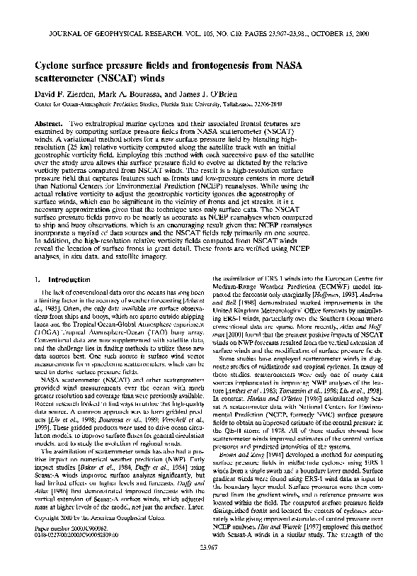:::::::::::::::::::::::: sensitivityto attenuationby liquid water was increased.Engineering advancementsin the sensorsincreasedthe signalto km noiseratio of the backscattermeasurements, greatlyimproving Figure 1. Data coverageandresolutionalongthe path of the ambiguityselection.In addition, each wind cell was viewed ADEOS. Dots mark the relativelocationof eachwind sample. from three different angles. The NSCAT radar was dualpolarized from one antenna, providing additional measurementsto aid in the ambiguityselection.NSCAT wasequipped 1000 0 1000 to measure backscatter on both sides of the satellite track, boundarylayerapproachwastwofold:(1) the surfacepressure doublingthe coverageof ERS-1, which viewed only on one field was derived almost exclusivelyfrom scatterometerdata, and (2) swathdata were used directly,without averagingin spaceor time. The drawbackwasthat pressures couldonlybe computedwithin the swathof wind data. A discussion of the accuracyof scatterometersurfacepressurefields is given by Zeng and Brown [1998]. These surfacepressurefields showed greatestimprovementover NWP analysesover the Southern Hemisphere,where the lack of conventionalobservations can causeentire systemsto be misplacedor missedall together [Brownand Levy, 1986;Levy and Brown, 1991]. This studymakesuse of the high-qualityNSCAT wind data by deducingsurfacepressurefieldsthroughthe use of a variational method. The primary goalsare (1) to use NSCAT windsto determinesurfacepressurefields,(2) to follow the side. A digital Doppler filter grouped overlappingbackscatter measurements from the differentviewinganglesinto 25 km by 25 km cells.The wind speedand directionwere computedfor each cell usingthe observedbackscattersand a lookup table. Calibration/validation of the NSCAT model function was more accuratethan previousscatterometersbecauseof comparisons with high-qualityin situ surface observationsfrom research vessels[Bourassaet al., 1997], National Data Buoy Center (NDBC) buoys[Freilichand Dunbar, 1999], and the TOGATAO array (K. Kelley and S. Dickenson,personalcommunication, 1998). In particular,thesein situ data includedmany observationsat low and high wind speeds,enablingaccurate calibration/validation and removingthe low wind speedbiases found in other scatterometers. Attenuationby liquid in the atmosphere,particularlyheavy precipitation, is a disadvantageof the Ku band frequency. vide a surfacepressurefield that could be used to improve Contaminationfrom precipitation droplets can significantly NWP over the oceans. degradethe quality of scatterometer-computed wind vectors. Section 2 describesthe data sets, including specificsof Ideally, inclusionof a passivemicrowaveradiometer on the satelliteplatformcouldhaveidentifiedcontaminatedcellsand NSCAT and its near-surface wind observations. Section 3 deflagged them appropriately.Unfortunately,missionspecificatails the variational method used to determine surfaceprestions and fundingdid not allow for suchan instrumentto be sures. The variational method involves the assimilation of relative vorticity computed from the NSCAT wind vectors. includedwith NSCAT, soit is difficultto identifycontaminated cells.Studiesare ongoingto determinethe effectsof precipiSurface fronts are located and identified in the relative vortictation on the overall accuracyof the NSCAT winds. ity field as localizedbandsof high relativevorticity(section The ADEOS was a low-altitude, Sun synchronous,near3.1.1).Thesefeaturesare verifiedasfrontsusingin situobserpolar orbiter.In thisorbit, NSCAT covered90% of the ice-free vations and visible GOES 9 imagery. Section4 usesNSCAT oceanevery2 days.The antennaconfigurationallowedwinds surfacepressurefieldsto follow a caseof cyclogenesis and a to be measured in 600 km wide swaths on each side of the caseof frontogenesisin the North Pacific.Resultsshowthat satellite,with a 400 km gap in the nadir view between the the NSCAT surfacepressurefields resolvethe structure of swaths(Figure 1). NSCAT2 level II wind data coveredswaths these featuresin more detail than the NCEP reanalyses.The on each side of the satellite, with each swath 24 cells wide. NSCAT pressurefieldsalsoagreebetterwith NSCAT windsas Theserowsof 24 cellswereperpendicularto the satellite'spath far as the location of cyclonecentersand the orientation of (Figure 1). horizontal pressuregradientsare concerned.Quantitatively, NSCAT provedto be a veryreliableinstrument,determining the NSCAT pressurefields comparewell with NCEP, espe- near-surface winds(calibratedto a heightof 10 m) more acciallynear the referencebuoysand where recentsatellitedata curatelyand with fewer aliasesthan previousscatterometers. are available. In the open oceanthe chancesof selectingan incorrectambievolution of surface features describedmostlywith NSCAT data, (3) to locateand identifysurfacefronts,and (4) to pro- ZIERDEN ET AL.: SURFACE PRESSURE FIELDS AND FRONTS FROM NSCAT WINDS 23,969 guitywerenegligible at windspeeds over8 m s-1 [Bourassa et al., 1997]. Below that thresholdthe chancesof incorrectambiguity selectionincreasedwith decreasingwind speed.The RMS difference between NSCAT and research vessel winds wasfoundto be 1.6m s-• forwindspeed(forwindspeeds >4 m s-•) and13ø for direction. Theyfoundno statistically significantbiasesat low or highwind speeds.Freilichand Dunbar [1999] supportedthese findingsin a comparisonto qualitycontrolledNDBC buoy observations. 2.2. E 40 ....... •65 •70 •75 •80 •85 •90 •95 200 •- 205 2•0 2•5 220 225 Longitude NCEP Reanalyses and NDBC Buoys NCEP reanalysismean sea level pressuresare used to ini- Figure 2. Typical daily coverageof NSCAT winds over the tialize the pressurefield and to update boundaryconditions. studyarea. Gapswithin the swathsindicatemissingdata. National Climate Data Center (NCDC) buoy locations are The NCEP mean sea level field is different from its surface markedwith a square. pressurefield, primarily over elevatedland surfacesand becauseof smallvariationsdue to the limited spectralresolution of the model. The NCEP mean sealevel pressurefield is the most accurate representationof surface pressuresover the vorticity is computedfrom the pressurefield. A variational ocean.Throughoutthe remainderof the text, the term "sur- methodsolvesfor a newgeostrophicstreamfunction,minimizface pressure"will applyto all pressurevalues,includingthe ing the differencebetweenthe new geostrophicvorticityand vorticitywhere satellitedata are present NCEP reanalysismean sealevel pressureproduct.The NCEP the old geostrophic mean sealevelpressuredata are availableon a 2.5øglobalgrid and minimizingthe differencebetweenthe new geostrophic at 6 hour intervals.A third data sourceis in situ surfacepres- vorticity and the old geostrophicvorticitywhere no satellite suresfrom NDBC buoys46003, located at latitude 51ø51'5"N data are present.The result is an updated surfacepressure and longitude 20ø5'3"E, and 51001, located at latitude field that capturesthe featuresfoundin the NSCAT vorticity. The treatmentof NSCAT relativevorticityas geostrophic ig23ø24'4"Nand longitude 197ø34'1"E. noresthe ageostrophy of surfacewinds,which can be significant in the vicinity of fronts and jet streaks.However, this 3. Methodology approximation is necessary in the absenceof upperair thermal 3.1. Method and Study Area A goal of this studyis to devisea techniqueof deriving surfacepressurefieldsfrom NSCAT winds,whichhavegreater coverageand better resolutionthan ERS-1 winds.Like Brown andZeng[1994],individualswathdataare used,preservingthe spatialresolutionand small-scalefeaturespresentin NSCAT winds. Unlike Brown and Zeng [1994], any data within the domainhas an influenceon the entire pressurefield. Also, the surfacepressurefieldwill evolvein timewith eachsatellitepass and massfields.Repeatingthe procedurewith eachnew pass of the satellite over the domain allows the field to evolve in time as dictatedby NSCAT data. The stepsof this procedure are described in detail in sections 3.2-3.6. 3.2. Computing Relative Vorticity NSCAT windsare of high spatialdensityand are locatedon a regular grid alignedwith the satellitepath; consequently, relativevorticityis easilycomputedusingcenteredfinite difover the domain. ferences.The speedand azimuthaldirectionof the winds are (u') and along-track(v') compoThe studyarea is the North PacificOcean between20ø and convertedto across-track 55øN latitude and between 165ø and 225øE longitude. It is nents in a coordinatesystemalignedwith the satellite track. largely free of land and ice (scatterometers only work over The relativevorticity[s at eachinteriorpointin the two swaths water) and large enough to capture synoptic-scale systems. is Midlatitude cyclonestrack throughthe region. Furthermore, ' - (u'i,j+l - u'i,j- O/Xy' , (]) i+l,j - Ui-l,j conventionaldata are sparse,and numericalweather prediction analysescanuseimprovementin this area.The studyarea where i denotescell positionacrossthe swath,j denotescell could expectto seethree to four passesof the satellitein the positionalong the swath,and x' and y' are across-trackand ascendingnode and another three to four passesin the de- along-tracklocations.Ax' and Ay' are twice the cell size and scendingnodeeachday(Figure2). All computations and anal- are computeddirectlyfrom the latitude and longitudeof the ysesare performedon a 0.25øgrid overthe domain,preserving correspondingdata pointsinsteadof beingheld constantat 50 the small-scalefeaturespresentin the high-resolutionNSCAT km. They varied between 49 and 51 km. If wind data are winds. missingat anyof the neighboringcells,the relativevorticityat The technique developed in this study builds on the that point is consideredmissing.Delunay triangulationand strengthsof Brownand Zeng [1994]and incorporatesthe vari- interpolation[Renka,1982] then transfersthe satelliterelative ationalmethodof Harlan and O'Brien[1986].The procedure vorticityonto the 0.25ø grid. (Plate 1) beginswith an NCEP meansurfacepressurefieldand The RMS differencein NSCATwindspeeds is -1.6 m s-• interpolatesit onto the 0.25ø grid over the domain. For each when comparedto in situ data [Bourassa et al., 1997;Freilich subsequentpassof the satelliteover the studyarea the two and Dunbar, 1999].This uncertaintypropagatesthroughrelaswathsof NSCAT wind data are assimilatedinto the pressure tive vorticitycalculationsand resultsin an uncertaintyin relafield. Although surfacepressureand winds are physicallydif- tivevorticity valuesof roughly1 x 10-4 S-•, similarin magferent data types,they are related throughvorticity. Relative nitude to maximumvaluesin strongsynoptic-scale systems. vorticity is computedin the swathsfrom NSCAT winds and However, this RMS uncertaintyin NSCAT wind speedsinthen interpolatedto the 0.25ø domaingrid, while geostrophic cludes both systematic biases and random errors in the 23,970 ZIERDEN ET AL.: SURFACE PRESSURE FIELDS AND FRONTS FROM NSCAT WINDS Beginwith initialpressurefield Updateboundaryconditions every 12 hours(NCEP) -::'I--Assimilate vorticity from };............. -• each newsatellite pass .--". ! with variational method ................ Computerelativevorticityfrom NSCAT winds Repeat for each newsatellitepass Updated pressurefield Plate 1. Methodologyof computingsurfacepressurefieldsfrom NSCAT winds. NSCAT winds and the in situ data. Since relative vorticity involvesthe differencein u and v components,most of the uncertaintyin relativevorticityis due to randomerror alonein the NSCAT winds.The consistency of NSCAT relative vorticity fieldswith surfacefeaturesand NCEP geostrophic vorticity suggests that the uncertaintyin the NSCAT relativevorticityis small(<1 x 10-s s-•) andthatrandomerrorsin theNSCAT winds are <0.7 m s-•. 3.3. Frontal Detection A secondaryresultof this studydealswith the strongsignature of surfacefronts in the relativevorticityfieldscomputed from NSCAT winds. The identification and location of fronts usingsatelliteremote sensinghas long been a topic of great interest. Visible and IR imagery has taught us a great deal about the structure and evolution of extratropicalcyclones [Carlson,1980;Browningand Roberts,1994].This type of imagery,however,hasone inherentdrawback.Broadcloudcover at higher levels obscuresfeatures at lower levels and at the surface.Only in well-organized,sharplydefined systemscan the approximatelocationof surfacefrontsbe found from such passivesensors.Katsaroset al. [1996] used parametersfrom active/passive microwavesensorsaboardSpecialSensorMicrowave Imager (SSM/I), Geosat, and ERS-1 satellitesto study the evolution of marine cyclones.They found that frontal zonescouldbe identifiedby large gradientsin the SSM/I integratedwater vapor.Unfortunately,thisparameteris a measure of water vaporover the entire atmosphericcolumnand cannot isolatefeaturesat the surface.The locationof fronts changes with height becauseof the sloped surfaceof the interface betweenair masses.Consequently,the integratedwater vapor can only identify a broad frontal zone representativeof many levels rather than a sharp line at the surface.Katsaroset al. [1996] also used Geosat and ERS-1 altimeter wind speedsto identify wind speedgradientsin the vicinity of fronts. These ZIERDEN 45 • ET AL.' • 30. SURFACE -- - • 170 175 FIELDS AND FRONTS FROM NSCAT WINDS 23 971 .- --<- z_- 25:. , •, 165 PRESSURE ••180 185 190 ,,•;• ........ 195 200 205 210 215 220 225 Vortici[y 10m/s - 10 - 5 - I 1 5 1.0 10 -• s-' Plate 2. NSCAT winds and relative vorticity from two satellite passesaround 1800 UTC, December 20, 1996.Isotherms(degreesCelsius)are from NCDC ship and buoy data (asterisksmark individualobservations).A cold front is identifiedby the band of high relativevorticity(red) in the right swaths. altimeter data were often obscuredby precipitationin the area of interest,especiallyin the frontal zones. Surfacefrontscanbe identifiedin NSCAT windsby changes in wind speedand direction.These changesare often subtle, though,making the exactlocationof a front difficult to determine by visual examinationof the wind fields.When relative vorticityis computedfrom NSCAT winds,however,even subtle changesin wind speedand directionlead to largevaluesof higherpressuremeet. Winds curvecyclonicallyin responseto the localizedpressureminimum,resultingin highpositiverelativevorticityvalues(in the NorthernHemisphere). Plotsof relativevorticityin the NSCAT swathsare presented showinglinear bands of high relative vorticity near-surface fronts.The dual swathsof NSCAT windsand relativevorticity (Plate 2) showa mature cycloneat 1800 UTC December20, 1996. The cycloneis centered near 38øN and 186øE, as evirelativevorticity(>1 x 10-4 s--l).Frontsarecharacterized by dencedby the circulationcenter and high relative vorticity relativelylow pressureat the boundarywhere air massesof values.Unfortunately,the cyclonecenteris in the gapbetween 5O :..-',.,;' .. .1.0. ... Plate 3. domain. Goes 9 visible imagery from 1800 UTC, December 20, 1996. Solid white lines mark the study 23,972 ZIERDEN 165 170 ET AL.: SURFACE PRESSURE FIELDS AND FRONTS FROM NSCAT WINDS 175 180 185 190 195 200 205 210 215 220 225 'Vortieity 10m/s -10 -5 -1 1 5 10 10-' s-' Plate 4. NSCAT winds and relative vorticity from two satellite passesaround 1800 UTC, January5, 1997. Isotherms(degreesCelsius)are from NCDC shipand bouydata (asterisksmark individualobservations). A warm front extendsform the cyclonecenter eastwardacrossthe northernportion of the domain. the two passesof the satellite,and its exactlocationcannotbe determined.A narrow band of high relative vorticity curves southeastwardfrom near the cyclonecenter, possiblycorrespondingto the changein winds along a cold front. Rough contoursof surfacetemperaturemade from National Climate Data Center (NCDC) ship and buoy observationsverify a temperaturedrop behindthis feature.Furthermore,GOES 9 visible imagery(Plate 3) showsa classiccoma head at the low-pressure centerand a bandof cloudiness alongthe trailing cold front These two independentdata sourcesconfirm that the highvorticityband is indeed a signatureof the cold front. Warm and stationary fronts have strong NSCAT relative vorticitysignatures similarto thoseof coldfronts,thoughwarm fronts are typicallyweaker. The NSCAT wind and relative vorticity fields from two passesof the satellite around 1800 UTC January5, 1997, are plotted in Plate 4. A developing cycloneis roughlycenterednear 40øN and 185øE,and a band of strong relative vorticity extendsnorth and east from the center along a stationaryfront. There is a dramaticwind shift alongthis feature, with windsfrom the northeaston the north side and from the southwest on the south side. Surface tem- perature contoursfrom NCDC surface observationsshow a Plate 5. GOES 9 visibleimageryfrom 1800UTC, January5, 1997.Solidwhite linesmark the studydomain. ZIERDEN ET AL.' SURFACE PRESSURE FIELDS AND FRONTS FROM NSCAT WINDS strongtemperaturegradientfrom the high-vorticityline northward. GOES 9 visibleimageryfrom the sametime (Plate 5) showsa smallcyclonenear 30øNand 210øW,whichis alsoseen asa concentrationof highrelativevorticityat the samelocation in Plate 4. North and westof the smallcycloneis a broad band 1 Outside the swaths V,j: g,j- gg0, of clouds that extends from 30øN and 185øW north and east acrossthe entire domain. This cloud band correspondswell with the band of high relativevorticityin Plate 4, confirming the presenceof a stationaryfront thatwasfirstidentifiedin the NSCAT relativevorticity.The NSCAT vorticityfield succeeds in locatingthe front with 25-50 km usingthe resolutionof the NSCAT windsand the width of the highvorticityband, which 23,973 where R is a reduction (6) factor needed to increase the NSCAT relativevorticityto a geostrophicequivalent. The NSCAT relativevorticityis a surfacevaluethat needsto be increasedto a geostrophicequivalentbefore it is blended with geostrophic vorticity. A simple method for relating geostrophicor gradientwindsto surfacewindsusesreductionis more exact than other satellite data sources. rotation factors:Geostrophicwinds are multiplied by a constant of 0.6-0.9, dependingon boundarylayer stability,and rotatedcounterclockwise 15ø-30ø[Clarkeand Hess,1975].Har3.4. Computing GeostrophicVorticity lan and O'Brien[1986]useda leastsquaresmethodto find an The variationalmethodrequiresNSCAT relativevorticityto averagereductionconstantof 0.83 and a rotation factor of be blendedwith the geostrophic vorticityof the initial pressure 27.6ø between geostrophicand Seasat-Awinds. Brown and field. Geostrophicvorticity is givenby Zeng [1994] used their boundary layer model to arrive at a 1 = reduction t3 +7 constant of 0.667 and a rotation factor of 18 ø for (2) neutral stratification.Herein R is chosento be 1.5, equivalent to Brownand Zeng'sreductionfactor for neutral stability.The wherep is the surfacepressure,p is taken as a constant1.225 rotation factor is inconsequentialsincerotatingNSCAT winds kgm-3 (U.S.standard atmosphere), f istheCoriolisparame- by a constantangle has no effect on relativevorticityvalues. ter,/3 - df/dy, andua isthezonalcomponent of thegeostro- The last term on the right of (3) is a penaltyfunctionthat phicwind. In centeredfinite differenceform, (2) becomes acts to smooth horizontally the solution field. Without this term the onlysolutionis X = 0, and satellitevorticityis inserted 1 directlyinto the field. In general,the penaltyfunctioninvolves ;•,•=• (P'+•'J +p,-•,j - 2pij)/Ax 2 the secondderivative of the solution field, often in the form of a Laplaciansmoother.In this case,however,the Laplacianof p is includedin the model, and another penaltyfunctionmust 1 - +•jj(Pi,j+l +Pi,j-1 be used.The kinematicgeostrophic kineticenergyG(pis) is minimized[Harlan and O'Brien,1986]: 13 f•2 (P,,j+• +Pi,;-O/2Ay (3) 1 1 G(pij) =• (tt2a + v})= 2--•Vp'Vp. Theinitialguess for •a iscomputed fromtheinitialNCEPgrid. (7) For each subsequentstep the pressurefields and all calculaThe coefficients K g and Ke are weightsthat controlthe tions are performedon the 0.25ø grid. balancebetweenthe amount of smoothingto be done and the data misfits. The cost function 3.5. Variational Method A variational method determinesan optimal surfacepressure field that smoothlyblendsNSCAT vorticityover the domain. The variational method minimizes the cost function F to findthe solutionfieldsPii and j K• KE + E E T (V'j)2 + E E TG(pii)' (4) i j to arrive at OF 1 Opijof(Xi+I'J -'1Xi-l'J2Aij)/z53c2 1 F(po •ij, X,•) =• • Xi;[ (• V2p fu i must be minimized thesolution field i j where the terms on the right-handside are summedover all grid pointsi and j. The first term on the right-handside is -+-•(Xi,j+I -+Xi,j_ 1--2Aij)/Ay 2 +p-• (Xi,j+• +Ai,j_O/2Ay p2f2 [(Pi+•,• +Pi-•,•PXi•)/Ax2 + (Pi,•+•+ pi,•-•- p Xi•)/AY 2]= 0 (8) commonly referredto asthemodel(•a = (1/Pf)V2P + OF (13/f)ua), the unknownpressure andvorticityfields,multipliedby a Lagrangemultiplier;t•i. Thisterm is knownas a Ogij Xijnt-i•Vij 0 (9) "strong constraint"[Saski, 1970]. The secondterm on the oF_(1 OXij -- • V2piJ +7 tta--gij =O. (10) right-hand sideminimizes thedatamisfitsVi•betweenthenew geostrophic vorticity•i• andsatellite vorticity (whereavailable) and the misfitsbetweenthe newand old geostrophic vorticities Equation(8) can be written as (outsidethe swaths). In the swaths +7 G = (11) 23,974 ZIERDEN ET AL.: SURFACE PRESSURE FIELDS AND FRONTS FROM NSCAT WINDS and has a solution because the feature of the form ,kij = •ppf (p,j- P0,j), of interest was located in the center of the studyarea. In the interior of the domain.thesolutionfield is looselyconstrainedby the boundaryvalues,so their solution (12) field realized the full influence of the assimilated scatterometer data over the low-pressuresystem.Also, they assimilatedsatwhereP0iiis thehomogeneous solution to (11) andthussatisfies (rE/2Pf)V2Poij= 0. Ontheboundaries, • = 0 and ellite data only oncefor eachNCEP analysis,so their solution field was not required to evolvein time. Poil - pij; therefore Poi•canbe foundthroughsuccessive Neumann boundaryconditionsare usedfor this study.The overrelaxationgiventhe boundaryvaluesfrom the initial prespressuregradientnormalto the boundary(asdeterminedfrom surefield. Combining(9) and (12) and lettingK = K•:/Kc NCEP reanalysis)is computedat each grid point along the leads to border.Equations(15) and (16) are then solvedholdingthese In the swath normal derivativesconstant. This approach allows surface K pressurevaluesto changewith the assimilationof NSCAT vorticity,evenat and near the borders.The drawbackof using derivativeboundaryconditionsis that the spatialmean pres- •,j= •s,j + •ppf (P,j-P00) Outside (13) the swath sure is not constrained: K •,;= •g,j + •ppf (P,; -P0•;). (14) Substitutionof (13) and (14) into (10) yields In the swath 1 1 The mean can drift from the initial value in a manner other than the true temporal evolutionof the mean.The horizontalgradientsand relativehighsand lows in the solution field are realistic, but while assimilatingone overpass,the spatialmean would drift between0 and 6 mbar from ground truth. Without additional measuresthis error addsup quicklyas the procedureis repeatedfor new satellite passes. p•)(Pi+l,j +P,-•,, - 2P•j)/Ax2 +• (Pi,j+l +Pi,j-1 - 2pij)/AY 2 The drift in spatialmean pressureis remediedwith refer13 K •;2 (Pi,j+l +pi,;_l)/2Ay - •ppf (p,; -Po•j) = ;s,, Outside (15) tures. A constant offset could then be added to or subtracted the swath 1 1 pfj(P,+i,; +P,-1,j2pij)/Ax2 +• (P,,;+i +P,,,-• --2p,)/ zXy 13 encepressures from within the domain.Ideally, the reference pointswouldbe locatednear the centerof the studyarea and awayfrom sharphorizontalpressuregradientsor extremefea- K from the solution pressurefield to make the solution and reference pressuresequal at the reference points. Unfortunately,buoysare onlylocatedin the domainby Hawaii andthe Aleutians, near the southern and northern borders of the do- main (Figure 2). The offset is taken as the averageof the differences between buoy and solution pressuresat these points.Averagingreducesthe influenceof the locationalerrors which are solvedusingsuccessive overrelaxationand constant in sharpgradientsnear the referencepoints. normal derivativeboundaryconditions. The derivativeboundaryconditionsstill presentlimitations Lagrange multipliers Ai•oftenhavea physical interpretation. on the evolution of features near the borders:Large-scale For example,in (9) the Lagrangemultipliersare equalto the features are not able to enter or leave the domain as the data misfits.Resultsshowthat their spatialdistributionis domsolutionfield evolvesin time. For example,considera lowinated by small-scalenoise,with variationsat 1 order of magpressuresystementeringthe domain on the westernborder. nitude less than averagevorticityvalues.No physicalstrucTo capturecorrectlythis feature as it crossesthe border,the tures,suchas the edgesof the satelliteswaths,are discernable normal derivativeshouldchangefrom positive(increasingtoin their spatialdistribution.The Lagrangemultiplierscorreward the interior) to negative.For this reasonthe boundary spondto grid-scalevorticitydifferencesbroughtaboutby the conditionsmustbe updatedperiodically.On the basisof dosmoothingterm in the variationalmethod. main size and the frequencywith which new passesof the A stated earlier, K is a coefficientthat weightsthe relative satellite occur, new derivativeboundary conditionsare comcontributions of the two constraints in the cost function. Furputed from NCEP reanalysesevery 12 hours. The 12 hour thermore, the two constraintsare not dimensionallyhomogeupdate cycleis chosenso that new boundaryconditionsare neous, and the coefficient must account for the difference in implementedat the synoptictimes of 0000 UTC and 1200 units in the two terms. A value of K = 1 x 10-•3 m-2 UTC. Using additional NCEP data to update the boundary producesa smoothpressurefieldwhilepreserving the physical conditionsdoesnot lessenthe dependencyof the solutionfield structurespresentin the NSCAT windsand relativevorticity. on NSCAT vorticitydata. It simplyprovidesa frameworkof Higher valuesput too muchweighton minimizingthe geostrolarge-scalehorizontalpressuregradientsto governthe solution phickineticenergy,resultingin a pressurefield with gradients near the borders. ff (P,,/+i +pi,;_l)/2Ay - •ppf (p,; -Po,;) = (16) that are too relaxed. 3.7. Viability of the Technique 3.6. Boundary Conditions and Reference Pressures Solving(15) and (16) for surfacepressurerequiresspecification of boundaryconditionson the bordersof the domain. Harlan and O'Brien [1986] held the boundarypressurevalues constant(Dirichlet), settingthem equal to the valuesfrom NCEP analyses.This conditionwas effectivefor their study A major goal of this studyis to describethe evolutionof cyclonesbasedprimarily on NSCAT observations. With the assimilationof data from each new passof the satellite,less informationis retained in the pressurefield from the initial NCEP analysis.In 24 hours,sevento nine passesof the satellite overthe domaincover•--75%of the area (Figure2). In 48 ZIERDEN ET AL.: SURFACE PRESSURE FIELDS AND FRONTS FROM NSCAT WINDS hours the total is over 90%, with a majority of the domain coveredat least twice. At this point the geostrophicvorticity field is describedalmostexclusivelyby NSCAT vorticity.The solutionpressurefield follows from the geostrophicvorticity field, constrainedonly by the pressurefield from the previous iteration, the derivativeboundaryconditions,and the two reference pressures. Continued assimilation of new satellite passes changesthe geostrophic vorticityfield (and corresponding pressurefield) as physicalfeaturesmoveaboutand evolve in the domain. Ideally, the processcontinuesthroughoutthe life cycleof the feature of interest. The techniquedoes,however,havetwo limitations.First, the feature (cyclone,front, etc.) must have a strongsignaturein the satellite vorticity field. Results show that high values of relativevorticityare concentratedat frontal zonesand cyclone 23,975 The first satellite pass covers only a small corner of the domain.The NSCAT pressurefield changesverylittle from the NCEP initialization,asidefrom smoothingthe discontinuities causedby NCEP's coarse 2.5ø grid (Figure 3a, 0000 UTC December18, 1996).This iteration demonstrateshow the field retainsthe characteristicsof the previousstepover areaswhere no new satellite information is available for assimilation. After the assimilationof eight passesthe NSCAT pressurefield evolvesconsiderably(1800 UTC, December 18, 1996). The low-pressuresystemnear the northern border weakens,while the low-pressuresystemnear the southernborder deepensin responseto the strongvorticity values from the last satellite pass.The NCEP analysisfrom the sametime doesnot intensify this system,yet showsa higher central pressure(1003 mbar comparedto 997 mbar) than the NSCAT field. Also, notice centers. If the feature is weak or diffuse, noise and small-scale how the isobarstend to "kink" where winds turn sharplyin variations in the NSCAT relative vorticity overwhelm the responseto featuresof high vorticity.Sharpbendsin pressure large-scalestructureof the feature. The solutionfield diverges contoursare indicativeof a suddenchangein horizontal grafrom the true surfacepressurefield, and this problem is com- dient, often associatedwith frontal zones[Djuri•5,1994]. At 1200 UTC, December 20, 1996, the cyclonereachesits poundedas more satellitepasseswith weak vorticitypatterns are assimilated.Also, cellscontaminatedby attenuationfrom maturestage(Figure 3c). The NSCAT centralpressureis 989 liquidwater introduceerror into the vorticityfield. These er- mbar, close to NCEP's value of 987 mbar. NCEP locates the rors do not appear to affect greatlythe solutionpressurefields center at 38øN and 186øE, 1ø east of the circulation center as for strongsystemsas the attenuationerrors are more local in determinedfrom the NSCAT wind vectors.The NSCAT presnature and may not influencethe large-scalestructureof the sure field places the center at 37øN and 185øE, 1ø east and pressurefield. It is impossible,however,to determinethe exact southof the circulationcenter.The only other differencein the impact of the attenuationproblem on the vorticity and pres- two pressurefieldsis that NSCAT buildshigherpressureat the surefieldswithout knowingwhich cellsare contaminated. northern edge of the domain, over 1050 mbar. The NCEP The techniquealsobreaksdownwhenthe featuremovestoo analysisonly has pressuresin this area of a little over 1040 quickly through the study area. Consider a cyclonemoving mbar. Elsewhere,the tow fieldsagreewell in the overallstrucwestto eastthroughthe domainat 10m s-•. On the firstday ture and the placementof major surfacefeatures.The NSCAT the satelliterecordsan area of high relativevorticitycorre- field hasbeen able to capturecorrectlythe intensifyingsystem spondingto the center at a longitudeof 175øE.This feature is with only the assimilationof NSCAT relative vorticity and assimilatedinto the pressurefield and resultsin a low-pressure updatedboundaryconditions. center at that location. The satellite may not pass over the By 1200UTC, December21, 1996(Figure4a), NCEP weakfeature again in 24 hours. Meanwhile, the true center of the ensthe systemto a centralpressureof 994 mbar. The cyclone cyclonewould have movednearly 800 km. If the satellitenow is now stretchedalonga major axisrunningnorthwestto southpassesover the center at its new positionwhile missingits old east.The centeris not well definedand is displacedfrom the position,the resultingpressurefield will erroneouslyshowthe circulationcenterby 5øto the north and 3øto the west.NSCAT feature as an elongatedor two-centeredsystem.The coverage keepsa central pressureof 987 mbar and correctlylocatesthe from NSCAT is insufficientto capturethe movementof the center at 38øN and 188øE, coincident with the center of circucycloneproperly,and the solutionfield divergesfrom the true lation of the NSCAT wind vectors.Both fieldshavetight prespressurefield. It is foreseenthat OuikSCAT, with its wider sure gradientson the northeastside of the cyclone,which coverageand no nadir gap,will alleviatemuchof this problem, agreeswell with the strong southeasterlywinds in this area. The orientationsof the NSCAT pressurecontoursare more particularlywhen multiple scatterometers are in operation. consistentwith the wind vectorsfrom the last satellitepass, especiallyjust north of the circulationcenter. 4. Case Studies Figure 4b depictsthe pressurefieldsat 1800 UTC, Decem4.1. Case 1: December 18-24, 1996 ber 22, 1996,after the assimilationof 40 satellitepassesover 5 The method is first applied to a case of cyclogenesis that days.The two pressurefields now agree on the cyclone'scenoccurredDecember18-24, 1996.The NCEP surfacepressure tral pressureof 993 mbar. NCEP correctlylocatesthe cyclone analysisfrom 0000 UTC, December 18, 1996, initializes the center at the center of circulation, while NSCAT has a double process.The solutionpressurefield (hereafter call NSCAT low. The tightestgradientsand strongestwindsare now on the pressure)evolveswith the assimilation of datafrom 52 satellite westernsideof the cyclone.Both fieldsalsoexhibitkinkingof passesover 7 days.Snapshotsof the NSCAT pressurefield are the isobarsalongthe coldfront, whichextendsto the southand comparedto NCEP reanalysesnearest in time to the latest east of the cyclonecenter. Two days later, at 1200 UTC, December 24, 1996, the cysatellitepass.Also, both the NSCAT and NCEP pressurefields are checked for consistencywith the NSCAT wind vectors clone reintensifieswith a central pressureof 992 mbar. The from the latest satellite pass.This comparisondoes not con- stormis large,nearlycoveringthe entire domain.NSCAT and stitutevalidationof the NSCAT pressurefields,asan indepen- NCEP are in good agreementwith both the location and indent data sourceis necessaryfor objectiveresults.It is simply tensityof the cyclonecenter,with NCEP being a little deeper intendedto showhow the NSCAT pressurefields conform to at 989 mbar. Both fields are consistent with the NSCAT wind features seen in the NSCAT wind fields. vectors. A warm frontal zone now extends eastward from the 23,976 ZIERDEN (a) ET AL.: SURFACE PRESSURE FIELDS AND FRONTS FROM NSCAT WINDS 0000UTC18 Dec.1996 0000 UTC 18 Dec. 1996 5O 45 4O 35 30 20 165 175 (b) , , 185 195 , 205 - , 215 225 165 175 1800UTC18Dec.1996 185 195 205 215 225 1800UTC18Dec.1996 40 30 25 165 175 (c) 185 195 205 215 225 165 175 1200UTC20 Dec.1996 185 1200 UTC 195 20 205 Dec. 215 225 215 225 1996 55 5O 45 4O 35 3O 25 2O 165 175 185 195 205 215 225 165 175 185 195 205 Figure 3. Case 1: NSCAT surfacepressurefield (mbar) after the assimilationof (a) 1, (b) 8, and (c) 20 satellitepasses: (left) NSCAT windvectorsfrom the lastsatellitepassand(right) concurrentNCEP reanalysis surfacepressures. cyclone'scenter. The NSCAT pressurefield resolvesthis feature sharplyas seen in the 995 and 1000 mbar contoursand strongpressuregradientsnormalto the front. The NCEP analysishas gentlycurvingcontoursin this zone, makingthe exact NSCAT low-pressurecenterlocationexactlymatchesthe center of circulation.NSCAT alsodoesa better job of showingthe elongatednature of the low, especiallyon the easternend. Notice how the wind vectors parallel the NSCAT pressure location contours of the front difficult to determine. in this area. NCEP does not extend the low far enougheast, as the wind vectorscrossthe contoursat unreal4.2. Case 2: January 3-6, 1997 isticallylarge angles,flowing from low to high pressure. This is a caseof frontogenesis that took placeduringJanuary The low moveslittle in the next 18 hours(Figure5c). The 3-6, 1997. The processis initialized at 0000 UTC, January3, center is now locatedat 49øN and 192øEin the NSCAT pres1997,when the only feature of interestis a weak low-pressure sure field, coincident with the center of circulation. NCEP systemcenteredat 48øNand 177øE(Figure 5a). The NSCAT pressurefield picksup anotherlow-pressurelobe enteringthe continuesto place the center too far to the east by 2ø. Both fieldshavea centralpressureof 983 mbar. The NCEP analysis domain on the western border at 40øN. This feature is not seen places another distinct low at 42øN and 172øE,where the in the NCEP reanalysis. NSCAT field has a more continuoustroughextendingeastto Figure 5b shows1800 UTC, January3, 1997.The low moves eastand, accordingto the NSCAT pressurefield, is centeredat westacrossthe northernportion of the domain.Sixhourslater, 50øN and 190øE with a central pressureof 994 mbar. The at 1800 UTC, January4, 1997, an apparentfront has formed NCEP analysisplaces the center 2ø south and east of the and extendsacrossthe northern portion of the study area NSCAT location with a central pressureof 987 mbar. The (Figure6a). The front in the NSCAT pressurefieldis defined ZIERDEN ET AL.: SURFACE PRESSURE FIELDS AND FRONTS FROM NSCAT WINDS (a) 165 1200UTC21 Dec.1996 175 (b) 185 195 205 215 1200UTC21 Dec.1996 225 165 175 1800UTC22 Dec.1996 551000' .' • 45 ' 35 30 25 175 (c) 185 1200 UTC 195 24 195 205 215 225 - '••' ,• ,•O• _ 20 165 185 1800UTC22 Dec.1996 • 5O 23,977 205 Dec. 215 225 165 175 185 1200 1996 UTC 195 24 205 Dec. 215 225 215 225 1996 50 45 40 30 20 165 175 185 195 205 215 225 165 175 185 195 205 Figure4. SameasFigure3 butfor theassimilation of (a) 29, (b) 40,and(c) 52 satellite passes. by a nearlycontinuous bandof highvorticityandlowpressure. nowcurvegentlyaroundthewesternsideof the centerrather North of the front, thewindsare east-northeast, while southof than shiftingsharplyas in earlierswaths.Also, beginningat the front, they are from the west-southwest. Also, pressure 1200UTC, January5, 1997,a newwindshiftline formsto the to the genesisof a gradients havetightened on bothsidesof thefront.Thewind southeastof the center, corresponding shift line coincideswell with the line of lowestpressures.The trailingcold front (Figure6b). This featureis seenin the fieldasa sharptroughextending southof the NCEP analysis persists in separating the featureinto two dif- NSCATpressure ferent lows. NSCAT wind vectors show no evidence of closed cyclone center.NCEPdoesnotresolve thefront,showing only isobars withthetroughaxisplaced10øeastof the circulation aroundeitherof the featuresto supportthisanalysis. gentlycurved The front is nearlystationaryfor the next 24 hoursand is NSCAT position. sharply delineated bythe 1800UTC, January 5, 1997,NSCAT 4.3. Accuracyof the NSCAT and NCEP PressureFields pressure field.Thewindshiftacross thefrontfromnortheast to Two generalizations canbe madeaboutthe NSCAT pressouthwest is highlylocalizedalongthe lengthof the front. NCEP finallymergesthe twolowsintooneelongated feature, sure field from these case studies. First, the field is more althoughit is not as linear as was depictedby the NSCAT realistic in the interior of the domain than near the boundaries. into pressure field.The NCEP analysis hasslightlylowerpressure New featuresmovinginto the domainare not assimilated (986mbar)thanNSCAT(989mbar)onthewestern portionof the NSCAT pressurefield until the satellitepassesoverthe the front. Otherwise,the NSCAT positionsof two smalllow- area, so thesefeaturesmay be totally missed.Also, regions pressure featuresalongthe front agreewell with the wind near the bordersare constrainedby the boundaryconditions. Awayfromtheborders, thesolution fieldisfreeto conformto circulationpatterns. At 1800UTC, January5, 1997,thewesternmost lobeof low featuresfound in the NSCAT relative vorticity.Second,the fieldismoreaccurate wherethesatellitehas pressure is developing intoa newcyclone (Figure6c).Winds NSCATpressure 23,978 ZIERDEN ET AL.' SURFACE PRESSURE FIELDS AND FRONTS FROM NSCAT WINDS (a) 0000UTC 3 Jan.1997 0000UTC 3 Jan.1997 45 25 10•m/s (b) 1800 UTC 3 Jan. 10•m/s 1997 1800 UTC 3 Jan. 1997 55 5O 45 4O 35 30 25 20 165 175 (C) 55 185 195 205 215 225 165 175 1200UTC 4 Jan.1997 185 195 205 215 225 1200UTC 4 Jan.1997 50 35 , z'.•,•';;,'-' , 165 175 185 195 205 215 225 165 175 _1020 , 185 195 205 215 225 Figure5. Case2: NSCATsurface pressure field(mbar)aftertheassimilation of (a) 1, (b) ?, and(c) 12 satellite passes: (left)NSCATwindvectors fromthelastsatellite pass and(right)concurrent NCEPreanalysis surfacepressures. passedmorerecently.It standsto reasonthat the portionof buoyobservations areusedbyNCEPin theirreanalyses, sothe the domain updatedwith newer informationis more current two are not independent.Second,the observations were made thanan areathathasnot seena satellitepassin manyhours. at the samesynoptictimesastheNCEP analyses. The NSCAT Table 1 addresses the accuracyof both the NSCAT and pressure field,however, mayhaveseenthelastsatellitepassas NCEP pressure fields.Threehourlysurfacepressure observa- far as _+3hoursof thesynoptic time.Also,theNSCATprestionsfrom shipsandbuoys(courtesyof the NCDC are com- surefieldoutsidetheareacovered bythelatestpassisbasedon paredto valuesfrom boththe NSCAT andNCEP pressure oldersatelliteinformation, 12-24hoursfromthe latestpass. fieldsfor eachsnapshot in Figures3-6. For eachcasethemean Yet anothersourceof errorin theNSCATfieldis thescarcity andstandard deviation of thedifference between thepressure of referencepressures. Only two buoyswere available,and fieldvaluesandthein situobservations arecomputed usingall these are both located in the eastern half of the domain. Inavailable observations for that time. These statistics are com- accuracies in the pressuregradientscausedby oldersatellite putedfor allobservations in theinteriorof thedomain(at least datalead to increasingerrorswith distancefrom the reference 5ø from the boundaries).The resultsshowthat the NCEP points.The resultthat NSCAT pressure fieldshavemeandifpressurefield is quantitatively moreaccuratethanthe NSCAT ferencesand standarddeviations only slightlyhigherthan field.The NSCATmeandifference rangesfrom0.1to 2.5mbar NCEP'sreanalysis productsupports the validityof the variain magnitude,and the standarddeviationis between2.4 and tional methodin derivingsurfacepressures from NSCAT 6.1 mbar.The NCEP meandifferenceis small,between0.1 and 1.2 mbar, and the standard deviation is -•5.8 mbar. NCEP winds. Althoughthe NSCAT pressures maynot be quantitatively should bemoreaccurate forseveral reasons. First,theshipand more accuratethan NCEP over the domain as a whole, the ZIERDEN (a) ET AL.' SURFACE PRESSURE FIELDS AND FRONTS FROM NSCAT WINDS 1800UTC4 Jan.1997 23,979 1800UTC4 Jan.1997 5O ""'1000'• ! -""'•--4,z'•90 '' 45 4.0 ._. • '"" oo 35 30 , 25 20 165 175 (b) 185 1200 UTC 195 205 5 Jan. 215 225 165 175 185 1200 1997 195 UTC 5 Jan. 205 215 225 215 225 215 225 1997 55 50 45 40 35 30 25 20 175 165 (c) 195 185 1800 UTC 205 5 Jan. 215 225 165 175 185 1800 1997 195 UTC 5 Jan. 205 1997 50 45 x•.., ,-•, 40 30 25 :,!: 20 175 165 185 195 205 215 225 165 175 185 ,J 195 205 Figure6. SameasFigure5 butfor the assimilation of (a) 18,(b) 22, and(c) 27 satellitepasses. qualitativeadvantages are seenin the detailedcomparisonsvorticityfieldsgivesrise to featuresin the NSCAT pressure fields that are blurred or not seenat all in the NCEP analyses. sharplydefined,and pressuregradientsare more consistent NSCAT is also better at placingthe low-pressurecenters made in sections 4.1 and 4.2. Features such as fronts are more withtheNSCATwinds.The improveddetailin the geostrophic correctlywith respectto the center of circulationof the Table 1. ComparisonWith SurfaceData NSCAT Mean Time and Date 1800UTC, Dec. 18 1200UTC, Dec. 20 1200UTC, Dec. 21 1800UTC, Dec. 22 1200UTC, Dec. 24 1800UTC, Jan.3 1200UTC, Jan.4 1800UTC, Jan.4 1200UTC, Jan.5 1800UTC, Jan.5 Interior Standard NCEP Mean Interior Standard Difference, Deviation, Difference, Deviation, mbar mbar mbar mbar -0.2 0.2 0.6 -0.1 0.2 1.2 0.2 0.0 -0.3 -0.2 1.7 4.2 3.2 1.4 2.2 5.8 4.7 4.3 2.5 3.0 -0.2 1.5 -0.7 -0.1 2.0 1.0 -0.2 -2.5 -0.8 2.0 2.4 6.1 6.1 6.0 3.3 6.1 5.5 5.4 4.6 4.1 Number of Observations 39 34 29 37 37 35 34 32 33 48 23,980 ZIERDEN ET AL.: SURFACE PRESSURE FIELDS AND FRONTS FROM NSCAT WINDS Table 2. Difference in the Locationsof Low-PressureCenters Compared to Centersof Circulation NSCAT Time and Date 1200 UTC, 1800 UTC, 1200 UTC, 1200 UTC, 1800 UTC, 1200 UTC, 1800 UTC, 1200 UTC, 1800 UTC, 1200 UTC, Dec. 20 Dec. 20 Dec. 21 Dec. 22 Dec. 22 Dec. 23 Dec. 23 Dec. 24 Jan. 3 Jan. 4 Average NCEP Latitude, deg. Longitude, deg. Distance, km Latitude, deg. Longitude, deg. Distance, km -2.0 0.0 0.0 -1.0 - 2.0 0.0 0.0 0.0 0.0 0.0 2.0 0.0 1.0 1.0 0.0 2.0 0.0 0.0 - 1.0 0.0 280 0 85 140 225 170 0 0 85 0 0.0 1.0 -3.0 5.0 0.0 0.0 0.0 0.0 - 1.0 0.0 2.0 1.0 3.0 3.0 0.0 2.0 0.0 0.0 2.0 2.0 170 140 420 600 0 170 0 0 200 170 - 0.8 0.7 100 0.2 1.5 190 from 0.1 to 2.5 mbar in magnitudewith a standarddeviation between2.4 and 6.1 mbar. NCEP pressurescompareslightly over the North Pacific makes the NSCAT wind vectors the best better,with mean differencesbelow 1.2 mbar in magnitudeand alternativefor determiningthe correctlocationof low-pressure standard deviationsbelow 5.8 mbar. The accuracyof the centers. Table 2 shows the difference in location of lowNSCAT pressure fields increasesnear the latest satellite pressure centers compared to circulation centers for times swaths and in the interior of the domain. when the circulation center is revealed in the latest satellite Qualitatively,the NSCAT pressurefieldsresolvethe strucpath. In 2 of the 10 casesboth NSCAT and NCEP agree ture of cyclonesand fronts more realisticallyand with greater exactlywith the NSCAT winds.In the first case,at 1200 UTC, detail than the NCEP analyses.The NCEP model and other December1996,the NSCAT low-pressurecenteris placed280 spectralmodelsgenerallyrepresentfronts as broad transition km from the circulationcenter.This displacementis causedby zones because of their coarse resolution. The NSCAT winds an older vorticitymaximumlying betweenthe two swathsof a and resultantsurfacepressurefieldsbetter representfrontsas new pass,givinga falsevorticitysignatureto the new NSCAT boundariesbecauseof their high spatialresolution.Also, the pressurefield (section 4.1). Other than this isolated case, centersof cyclonesare placed more accuratelyin the NSCAT NSCAT low-pressurecenters are consistentlycloser to the pressurefieldsthan in NCEP analyseswhen comparedto the circulation centers than NCEP. On average, NSCAT low- centersof circulationfrom NSCAT winds.The averagedifferpressurecentersare 100 km from the circulationcenter,while ence is 100 km for NSCAT pressurefields and 190 km for NCEP averages 190 km errors. And interesting feature of NCEP analyses. Another resultof this studyis the signatureof surfacefronts Table 2 is the trend in longitudinalerror of the NCEP analyses. In 7 out of the 10 casesthe NCEP center is placed too far in relative vorticity fields computed from NSCAT winds. eastwardwhen comparedto circulationcentersand in no case Fronts are clearly identified by linear bandsof high relative is it displacedto the west.While 10 cases(two different sys- vorticityvalues.These bandsare verified as fronts usingsurtems) are too few to suggesta systematicbias in the NCEP face temperaturegradientsand satelliteimagery.NSCAT vorticity fieldslocatethe frontswith an accuracyof 25-50 km and analyses,the trend warrantsfurther investigation. with greater resolutionthan other satellitedata sources. Although NSCAT winds are a high-qualitydata source,ef5. Conclusions fective techniquesfor assimilationinto NWP models have A variationalmethodis devisedto generatesurfacepressure proven difficult to develop. Surface pressure fields from fields from NSCAT winds. The method solves for a surface NSCAT winds, however,could provide a more favorableaspressurefield by smoothlyblendingrelativevorticitycomputed similation source [Hoffman, 1993; Atlas, 1997]. This study from NSCAT windswith ambient geostrophicvorticity.The bringsforth a simplemethodfor determiningsurfacepressures method ignoresthe ageostrophyof surfacewinds as no upper from NSCAT winds and demonstrates its effectiveness. air thermal or massfieldsare usedto make adjustments.The solutionpressurefield is updatedasnew passesof the satellite Acknowledgments. Fundingfor thisprojectis from the NASA JPL over the studyarea provide additionalinformation.Neumann NSCAT project. COAPS receivesits basefundingfrom ONR's Secboundaryconditions,updatedtwice daily with NCEP normal retary of the Navy Grant to JamesJ. O'Brien. gradients,allow the surfacepressurefield to evolvein time. This method is used to studya caseof cyclogenesis and a caseof frontogenesisin the North Pacific.The NSCAT pres- References surefieldscorrectlycapturethesefeaturesasthey intensifyand Andrews,P. L., and R. S. Bell, Optimizing the United Kingdom MeteorologicalOffice data assimilationof ERS-1 scatterometer winds, move throughthe studyarea. The NSCAT pressurefieldsare Man. WeatherRev., 126, 736-746, 1998. qualitativelycomparedto NCEP reanalysissurfacepressure Anthes,R. A., V. H. Kuo, andJ. R. Gyakum,Numericalsimulationsof fields, and both fields are quantitativelycomparedto NCDC a case of explosivemarine cyclogenesis, Man. WeatherRev., 111, ship and buoy observations.The domain-averageddifferences 1174-1188, 1983. between NSCAT pressuresand surfaceobservationsrange Atlas, R., Atmosphericobservationsand experimentsto assesstheir NSCAT winds. An independentdata sourcewould lead to a more objectivecomparison,but the lack of conventionaldata ZIERDEN ET AL.: SURFACE PRESSURE FIELDS AND FRONTS FROM NSCAT WINDS usefulnessin data assimilation,J. Meteorol. Soc. Jpn., 75, 111-130, 1997. Atlas, R., and R. N. Hoffman, The use of satellite surface wind data to 23,981 winds:Comparisonswith National Data Buoy Center buoys,J. Geophys.Res., 104, 11,231-11,246,1999. Harlan, J., Jr., and J. J. O'Brien, Assimilation of scatterometer winds improveweatheranalysisandforecasting, in Satellites, Oceanography into surfacepressurefields usinga variational method,J. Geophys. Res., 91, 7816-7836, 1986. and Society,pp. 57-79, Elsevier,New York, 2000. Atlas, R., E. Kalnay, and M. Halem, Impact of satellitetemperature Hoffman, R. N., A preliminary study of the impact of the ERS-1 soundingsand wind data on numerical weather prediction. Opt. C-band scatterometerwind data on the European Centre for MeEng., 24, 341-346, 1985. dium-RangeWeather Forecastsglobal data assimilationsystem,J. Baker, W. E., R. Atlas, E. Kalnay, M. Halem, P.M. Woiceshyn,S. Geophys.Res.,98, 10,233-10,244,1993. Peteherych,and D. Edelmann, Large-scaleanalysisand forecast Hsu, C. S., and M. G. Wurtele, Constructionof marine surfacepressure fields from scatterometerwinds, J. Geophys.Res., 36, 1249experimentswith wind data from the Seasat-A scatterometer,J. 1261, 1997. Geophys.Res., 89, 4927-4936, 1984. Bourassa,M. A., D. M. Legler, and J. J. O'Brien, NSCAT winds Katsaros,K. B., J. M. Adams, and N.M. Mognard, Evolution of two oceanicextratropicalcyclonesas observedwith the specialsensor validationwith researchshipobservations, Eos Trans.AGU, 78(17), microwaveimagerand the Geosatand ERS-1 altimeters,J. Geophys. SpringMeet. Suppl.,S76, 1997. Bourassa, M. A., L. Zamudio, and J. J. O'Brien, Noninertial flow in NSCAT observationsof TehuantepecWinds,J. Geophys.Res.,104, 11,311-11,319, 1999. Brown, R. A., and G. Levy, Ocean surfacepressurefields from satel- Res., 101, 6627-6639, 1996. Levy, G., and R. A. Brown, SouthernHemispheresynopticweather from a satellite scatterometer,Mort. WeatherRev., 119, 2803-2813, 1991. lite-sensed winds, Mon. WeatherRev., 114, 2197-2206, 1986. Liu, W. T., W. Q. Tang, andP.S. Polito,NASA scatterometerprovides Brown, R. A., and L. Zeng, Estimatingcentral pressuresof oceanic global ocean-surfacewind fieldswith more structuresthan numerimidlatitudecyclones,J. Appl. Meteorol.,33, 1088-1095, 1994. cal weatherprediction,Geophys. Res.Lett., 25, 761-764, 1998. Browning,K. A., and N.M. Roberts,Structureof a frontal cyclone, Renka, R., Interpolationof data on the surfaceof a sphere,Oak Ridge Q. J. R. Meteorol. Soc., 120, 1535-1557, 1994. Natl. Lab. Rep. OLNR/CSD-108, Oak Ridge Natl. Lab., Oak Ridge, Tenn., 1982. Carlson,T. N., Airflow throughmidlatitudecyclonesand the comma cloud pattern, Mon. WeatherRev., 108, 1498-1509, 1980. Saski, Y., Some basic formalismsin numerical variational analysis, Mort. WeatherRev., 108, 875-883, 1970. Clarke, R. H., and G. D. Hess, On the relation between surfacewind and pressuregradient, especiallyin the lower latitudes,J. Phys. Tomassini, M., D. LeMeur, and R. W. Sounders,Near-surface satellite Oceanogr.,9, 325-339, 1975. wind observationsof hurricanesand their impacton ECMWF model Djuri6, D., WeatherAnalysis,304 pp., Prentice-Hall,EnglewoodCliffs, analysesand forecasts,Mort. WeatherRev.,126, 1274-1286, 1998. N.J., 1994. Vetscheil, M. A., M. A. Bourassa,D. E. Weissman, and J. J. O'Brien, Model validation of the NASA scatterometerwinds, J. Geophys. Duffy, D. G., and R. Atlas,The impactof Seasat-Ascatterometerdata Res., 104, 11,359-11,373, 1999. on the numerical prediction of the Queen Elizabeth II storm, J. Geophys.Res., 91, 2241-2248, 1986. Zeng, L. X., and R. A. Brown,Scatterometerobservations at highwind Duffy, D., R. Atlas, T. Rasmond,E. Barker, and R. Rosenberg,The speeds,J. Appl. Meteorol.,37, 1412-1420, 1998. impact of Seasat scatterometerwinds on the Navy's operational model, J. Geophys.Res.,89, 7238-7244, 1984. M. A. Bourassa, James J. O'Brien, and D. F. Zierden, Center for Freilich, M., and R. S. Dunbar, A preliminaryC-band scatterometer Ocean-AtmosphericPredictionStudies,Florida State University,Talmodel functionfor the ERS-1 AMI instrument,paper presentedat lahassee,FL 32306-2840.(zierden@coaps.fsu.edu) First ERS-1 Symposium,European SpaceAgency,Cannes,France, 1992. (ReceivedMarch 22, 1999;revisedFebruary14, 2000; Freilich, M., and R. S. Dunbar, The accuracyof NSCAT 1 vector acceptedMarch 20, 2000.)