Flow Assurance Management and Benchmarking: Slugging, Hydrate and Wax Formation Assessment of an Offshore Oil Field. Flow Assurance Management and Benchmarking: Slugging, Hydrate and Wax Formation Assessment of an Offshore Oil Field. Abstract Over the years, the desire of oil and gas operators to reduce topside facilities using Subsea Production Systems (SPS) has increased tremendously. This has resulted in the overwhelming importance of flow assurance studies in ensuring the SPS delivers the produced fluid to the production platform at the desired operating conditions for surface facilities while still meeting the production ambition of the oil and gas operator. This paper will illustrate how flow assurance management and benchmarking for slugging, hydrate and wax formation was achieved for an offshore oil field. Furthermore, it concludes by recommending operational modes which should be addressed prior to finalising the pipeline architecture by proposing possible approaches to maximizing production for the field under study. Key Words: Slugging, Hydrates, Wax, Overall Heat Transfer, Insulation, Pressure Loss, Vapour Quality, Multiphase Flow 1.0 Introduction The field under study consists of the exploitation of an associated gas, dry oil reservoir with no significant water production expected in its first 3 years of operation. The operator is desirous of producing this reservoir using a drill centre consisting of four (4) wells, each anticipated to have a liquid production rate of 820 (standard) sm3/day which ultimately translates to a peak production rate/throughput from the four wells to be 3,280 sm3/day. The production wells will be linked to a clustered production manifold using jumper /tie-in spools. 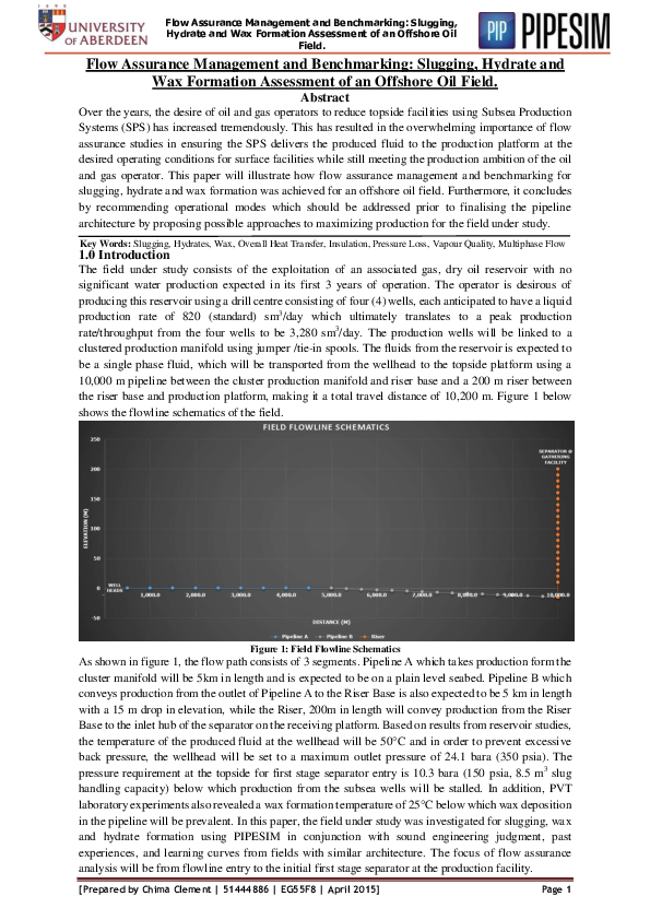The fluids from the reservoir is expected to be a single phase fluid, which will be transported from the wellhead to the topside platform using a 10,000 m pipeline between the cluster production manifold and riser base and a 200 m riser between the riser base and production platform, making it a total travel distance of 10,200 m. Figure 1 below shows the flowline schematics of the field. Figure 1: Field Flowline Schematics As shown in figure 1, the flow path consists of 3 segments. Pipeline A which takes production form the cluster manifold will be 5km in length and is expected to be on a plain level seabed. Pipeline B which conveys production from the outlet of Pipeline A to the Riser Base is also expected to be 5 km in length with a 15 m drop in elevation, while the Riser, 200m in length will convey production from the Riser Base to the inlet hub of the separator on the receiving platform. Based on results from reservoir studies, the temperature of the produced fluid at the wellhead will be 50°C and in order to prevent excessive back pressure, the wellhead will be set to a maximum outlet pressure of 24.1 bara (350 psia). The pressure requirement at the topside for first stage separator entry is 10.3 bara (150 psia, 8.5 m3 slug handling capacity) below which production from the subsea wells will be stalled. In addition, PVT laboratory experiments also revealed a wax formation temperature of 25°C below which wax deposition in the pipeline will be prevalent. In this paper, the field under study was investigated for slugging, wax and hydrate formation using PIPESIM in conjunction with sound engineering judgment, past experiences, and learning curves from fields with similar architecture. The focus of flow assurance analysis will be from flowline entry to the initial first stage separator at the production facility. [Prepared by Chima Clement | 51444886 | EG55F8 | April 2015] Page 1 Flow Assurance Management and Benchmarking: Slugging, Hydrate and Wax Formation Assessment of an Offshore Oil Field. 2.0 Base Data Multicomponent mixture characterizations of reservoir fluids which exist as complex hydrocarbons are important to petroleum processes in order to be able to provide accurate fluid description, present solutions to improve compositional analysis and aid in system design. It is also a basis for the economics of projects with accurate phase behavior predictions as a major objective [1]. The subsequent subsections below gives a detailed description of the fluid composition for the field under study and attempts to recommend the appropriate line sizing based on boundary conditions to be utilized at the initialization of hydrocarbon production from the field. 2.1 Fluid Composition The fluid composition for the field under study consist predominantly of a compositional oil model. Table one below shows the fluid composition of the hydrocarbon to be produced. Water cut is anticipated to be initially 0% for the first three years of its production, thereafter increasing up to 90% during the field’s productive life. Table 1: Compositional Fluid Properties at Inlet Conditions (@ 0% Water Content) Components Boiling Point °C Methane (C1) Ethane (C2) Propane (C3) Iso-Butane (IC4) Butane (NC4) Iso-Pentane (IC5) Pentane (NC5) Hexane (NC6) -161.49 -88.60 -42.04 -11.72 -0.50 27.84 36.07 68.73 C7+ 101.1 H2O Mixture Property 100 -9.56 Molecular Critical Mole Specific Weight Temperature Gravity % g/mole °C Pure Hydrocarbon Components 16.043 0.424 36.50 -82.57 30.070 0.546 4.40 32.17 44.096 0.584 2.60 96.68 58.123 0.597 0.63 134.99 58.123 0.616 0.13 151.97 72.150 0.618 0.67 187.25 72.150 0.624 0.83 196.55 86.177 0.658 2.70 234.45 Petroleum Fraction Component 115.000 0.683 51.54 268.00 Aqueous Component 18.015 1.000 0.00 373.98 71.45 0.5776 1.00 122.18 Critical Pressure Bar Acentric Factor 45.99 48.72 42.48 36.48 37.96 33.80 33.70 30.25 0.0115 0.0995 0.1523 0.1770 0.2002 0.2279 0.2515 0.3013 25.64 0.3462 220.55 34.85 0.3449 0.2041 Figure 2: Phase Diagram for Hydrocarbon Composition at Initial Condition [Prepared by Chima Clement | 51444886 | EG55F8 | April 2015] Page 2 Flow Assurance Management and Benchmarking: Slugging, Hydrate and Wax Formation Assessment of an Offshore Oil Field. Using the hydrocarbon fluid composition presented in table 1, PIPESIM was used to model the phase diagram of the hydrocarbon system as presented in figure 2. Further interpretation of the phase envelope revealed the following fluid properties for the hydrocarbon compositional fluid; Critical Temperature, � = 229.24°C Critical Pressure, � = 75.17 bara Cricondenbar, � = 104.69 bara Cricondentherm, � �= 234.98°C 2.2 Stock Tank Component Phase Split and Thermodynamic Properties Very key to ensuring a successful flow assurance management operation is understanding the thermodynamic properties for each phase of the fluid at inlet conditions. Based on the output of the compositional fluid components modelled in PipeSim, table 2 below presents the stock tank components and phase split volume for each of the components. Table 2: Stock Tank Component Phase Split and Thermodynamic Properties (@ 0% Water Content) Components Methane (C1) Ethane (C2) Propane (C3) Iso-Butane (IC4) Butane (NC4) Iso-Pentane (IC5) Pentane (NC5) Hexane (NC6) C7+ H2O Total Mole (%) Vapour Liquid 79.779 0.520 9.247 0.371 4.836 0.741 0.938 0.374 0.168 0.098 0.513 0.800 0.518 1.089 0.605 4.442 3.396 91.565 0.000 0.000 100 100 Thermodynamic Properties Mass Rate (kg/s) Density (kg/m3) Viscosity (Pa.s) Enthalpy (J/Mol) Entropy (J/Mol.K) Thermal Cond (W/m.K) Isobaric Heat Cap (J/Mol.K) Isochoric Heat Cap (J/Mol.K) Compressibility Joule Thompson Coef. (K/Pa) Gas Liquid Ratio (sm3/sm3) Phases Vapour Liquid 4.82 27.41 1.00 722.11 -5 1.0453 ×10 4.9937 × 10-3 -474.74 -37,271.06 5.0841 -99.76 0.0350 0.1000 46.27 227.02 37.78 201.09 0.9949 0.0065 -6 7.7560 × 10 -4.8386 × 10-6 127.15 2.3 Bubble Point Pressure and Dew Point Pressure Estimating the bubble point and dew point temperature and pressure of the hydrocarbon component is very vital because it provides key information on the phase behavior of the compositional hydrocarbon fluid at certain pressures and temperatures. The bubble point is the corresponding pressure and temperature at which the first bubble of gas is evolved from the hydrocarbon when in a single phase liquid state at operating conditions of temperature and pressure. Similarly, the dew point pressure is the corresponding temperature and pressure at which the first droplet of liquid condenses from the hydrocarbon when in a single phase gaseous state at operating conditions of pressure and temperature. Using the Wilson expression as shown in equation 2.1, a manual calculation was done on Microsoft™ Excel to calculate the bubble point and dew point temperature & pressure of the compositional hydrocarbon fluid. The Wilson’s equation is expressed as; � = Where ��− �−� � − −� �� � [ . � � +�� − ° �� ] . ° [Prepared by Chima Clement | 51444886 | EG55F8 | April 2015] Page 3 Flow Assurance Management and Benchmarking: Slugging, Hydrate and Wax Formation Assessment of an Offshore Oil Field. Table 3: Bubble Point Temperature Calculation @ Wellhead Conditions Ki Mole Fraction Components Xi Methane Ethane Propane i-Butane n-Butane i-Pentane Pentane Hexane C7+ Total 0.3650 0.0440 0.0260 0.0063 0.0013 0.0067 0.0083 0.0270 0.5154 1.00 Pc Bar Tc °K Accentric Factor 45.99 48.72 42.48 36.48 37.96 33.8 33.7 30.25 25.64 190.43 305.17 369.68 407.99 424.97 460.25 469.55 507.45 541.00 0.0115 0.0995 0.1523 0.177 0.2002 0.2279 0.2515 0.3013 0.3462 P Bar 24.1 Ki Xi Ki Ki Xi Temperature °K 213 3.3932 0.1571 0.0186 0.0046 0.0026 0.0007 0.0004 0.0001 0.0000 203 1.2385 0.0069 0.0005 0.0000 0.0000 0.0000 0.0000 0.0000 0.0000 1.2460 2.6713 0.1035 0.0110 0.0026 0.0014 0.0003 0.0002 0.0000 0.0000 0.9750 0.0046 0.0003 0.0000 0.0000 0.0000 0.0000 0.0000 0.0000 0.9799 From table 3 above, the bubble point temperature at the inlet condition of the wellhead was calculated to be, = ° ≈ − . ℃ with a corresponding bubble point pressure from the phase envelope to be, � = . . Table 4: Dew Point Temperature Calculation @ Wellhead Conditions Ki Components Mole Fraction Yi Pc °K Tc Kelvin Accentric Factor Methane Ethane Propane i-Butane n-Butane i-Pentane Pentane Hexane C7+ Total 0.365 0.044 0.026 0.0063 0.0013 0.0067 0.0083 0.027 0.5154 1.00 45.99 48.72 42.48 36.48 37.96 33.8 33.7 30.25 25.64 190.43 305.17 369.68 407.99 424.97 460.25 469.55 507.45 541.00 0.0115 0.0995 0.1523 0.177 0.2002 0.2279 0.2515 0.3013 0.3462 P Bar 24.1 Yi/Ki Ki Yi/Ki Temperature °K 493 53.5093 19.1708 8.2868 4.5015 3.8332 2.1734 1.9251 1.0227 0.5263 498 0.0068 0.0023 0.0031 0.0014 0.0003 0.0031 0.0043 0.0264 0.9793 1.0271 54.6484 19.8873 8.6820 4.7443 4.0530 2.3119 2.0528 1.0993 0.5699 0.0067 0.0022 0.0030 0.0013 0.0003 0.0029 0.0040 0.0246 0.9043 0.9494 From table 4 above, the dew point temperature at the inlet condition of the wellhead was calculated to be, = . ° ≈ . ℃ with a corresponding dew point pressure from the phase envelope to be, � = . . 3.0 Methodology Using the pipeline architecture and compositional fluid base data discussed in the previous sections, detailed analysis was carried out to determine the adequate riser and pipe sizing required to meet the desired pressure demand at the topside whilst taking into account the erosional velocity of the flowing stream in accordance with API RP 14E [2, p. 24]. Furthermore, using the outputted data presented by PIPESIM (see appendix I) and in conjunction with sound engineering judgment and past technical articles on the subject, further kinematic properties of the fluid were established. It is noteworthy that this analysis is concerned with only fluid transportation from the production manifold on the seabed to production platform at the surface. In addition, it has not taken into account pressure losses due to the effects of fittings and bends in the system due to unavailability of key subsea hardware data. 3.1 Riser and Pipeline Sizing The first task here is to establish the pipeline and riser sizing in order to achieve the desired production rate. This was done by performing a series of sensitivity analysis for the three (3) available pipeline sizes (0.241 m, 0.292 m, and 0.343 m) on a case by case bases from the minimum through to maximum anticipated production throughputs (3280, 2460, 1640 and 820) sm3/day. As mentioned earlier and [Prepared by Chima Clement | 51444886 | EG55F8 | April 2015] Page 4 Flow Assurance Management and Benchmarking: Slugging, Hydrate and Wax Formation Assessment of an Offshore Oil Field. based on the reservoir data provided, the field is expected a have a maximum water cut of 90% throughout its entire life with negligible water production for the first 3 years of its operation. The inlet pressure and temperature was fixed to 24.1 bar and 50°C respectively. The correct pipe sizing should be one with the minimum pressure drop at the riser base. The values for outlet pressure at the riser base was computed from the pressure/distance plot (see appendix 1.2 and 1.4). The sensitivity analysis was performed over the range of pipe diameters available at different production rates. The results are presented in tables 5 and 6 and the plotted curves in figures 3 and 4. Table 5: Sensitivity Analysis for Pipe Sizing @ 0% Water Cut Table 6: Sensitivity Analysis for Pipe Sizing @ 90% Water Cut As shown in tables 5 and 6 and figures 3 and 4, the pipe ID with the lowest pressure drop is 0.343 m. Figure 3: Plot of Pipe ID Vs. Outlet Pressure @ 0% Water Cut Figure 3: Plot of Pipe ID Vs. Outlet Pressure @ 90% Water Cut Further justification to the choice of line size is in accordance to API RP 14E sizing criteria for gas/liquid two phase lines which stipulates that flowlines transporting gas and liquid in two phase flow should be sized primarily on the basis of flow velocity. The velocity above which erosion may occur is determined using the following empirical equation [2]; . = . . √ Where c is an empirical constant and ρm is the no slip gas/liquid mixture density at flowing pressure and temperature expressed in kg/m3. Ve which is the erosional velocity is expressed in m/sec. For continuous service and assuming a solids free fluid, the empirical constant c is given as 100 m5/2 sec-1 kg-1/2. Results from output files (see appendix 1.1 and 1.3) of the computational fluid dynamics (CFD) simulation carried out using PipeSim reported a maximum no slip liquid hold up fraction � of 0.24 at 0% water cut and 0.79 at 90% water cut. These values are maximum at the lowest production throughput (820 m3/day) and around the riser base. The no slip mixture density can be calculated from the gas � and liquid density as; = � + −� � . . Similarly, the phase densities are maximum for the lowest production throughput and at the riser base (see appendix 1.1 and 1.3). Using equation 3.2, the no slip mixture densities were calculated to be 174.77 kg/m3 and 768.49 kg/m3 for 0% and 90% water cut respectively (see appendix III). Substituting these values into equation 3.1 gave a projected value of 9.22 m/sec and 4.4 m/sec for erosional velocity at 0% and 90% water cut respectively (see appendix IV). For the selected pipe ID of 0.343 m and in accordance with results from the summary file of the CFD simulation (see appendix 1.2 and 1.4), the mixture velocity of the hydrocarbon fluid at maximum throughput of 3280 sm3/day was found to be 2.9 m/sec (< 9.22 m/sec) and 0.9 m/sec (<4.4 m/sec) for 0% and 90% water cut respectively (see appendix [Prepared by Chima Clement | 51444886 | EG55F8 | April 2015] Page 5 Flow Assurance Management and Benchmarking: Slugging, Hydrate and Wax Formation Assessment of an Offshore Oil Field. 1.2 and 1.4). This is less than the erosional velocity earlier stated. Thus, it can be concluded that the identified line size is acceptable from an erosion viewpoint in accordance with API RP 14E. A summary of result for the erosional velocity criteria is presented in table 7 below. Table 7: Summary of Results for Justification That Erosional Velocity Criteria was satisfied. Erosional Velocity (API RP 14E) Mixture Velocity @ 3280 sm3/day 0% Water Cut 90% Water Cut 0% Water Cut 90% Water Cut 0.343 m 9.22 m/sec 4.40 m/sec 2.9 m/sec 0.9 m/sec Furthermore, the erosional velocity ratio which is the ratio of the fluid velocity at operating conditions to erosional velocity can be plotted against the flowline distance to show likely points of erosion in the system. Line Size Figure 5: Erosional Velocity-Distance Profile @ 0% Water Cut Figure 6: Erosional Velocity-Distance Profile @ 90% Water Cut As depicted in figures 5 and 6, an erosional velocity ratio less than 1 signifies an erosion free system. 3.2 Pressure/Temperature – Distance Profile The pressure/temperature distance profile gives us an overview for areas of major concern in the system that might need to be redesigned in order to minimize and/or prevent wax and hydrate formation in the system. The figures below shows the pressure/temperature – distance profiles of the pipeline system. Figure 7: Pressure-Distance Profile @ 0% Water Cut Figure 9: Temperature-Distance Profile @ 0% Water Cut Figure 8: Pressure-Distance Profile @ 90% Water Cut Figure 10: Temperature-Distance Profile @ 90% Water Cut [Prepared by Chima Clement | 51444886 | EG55F8 | April 2015] Page 6 Flow Assurance Management and Benchmarking: Slugging, Hydrate and Wax Formation Assessment of an Offshore Oil Field. As depicted in figures 7 and 8, the pressure- distance profile for 0% water cut meets the pressure requirement of a minimum of 10.3 bars at the topside for all production throughput. However, at 90% water cut, the outlet pressure seem to be below the minimum requirement of 10.3 bars for all production throughput. This is not a favorable condition for production optimization. PVT laboratory experiments also revealed a wax appearance temperature (WAT) of 25°C below which wax deposition in the pipeline will be prevalent. Figures 9 and 10 shows a system highly vulnerable to wax formation most especially from half way down the travel distance to the topside for all anticipated production throughput. The system has to be redesigned to prevent wax and hydrate formation during its operation. 4.0 Results and Discussions In accordance to the base data highlighted so far in the previous sections, we will now suggest solutions to redesigning the system in order to prevalent unfavorable operating phenomena such as wax, hydrate and slugging. 4.1 Wax and Hydrate Management Risk of wax and gas hydrates occurring in subsea flowlines presents problems to offshore oil and gas production operations. Hydrates and wax can occur in oil and gas flowlines provided that the favorable compositional mix and thermodynamic conditions exist [3]. Several correlations have been useful in predicting hydrate formation in compositional fluids. The most reliable one requires a compositional analysis. The Katz method utilizes vapor solid equilibrium constants defined by; � � = � . . Where � is the vapor solid equilibrium constant, � is the mole fraction in the liquid phase and � is the mole fraction in the vapor-phase. For calculation purposes all molecules too large to form hydrates have a k-value of infinity. These include normal paraffin hydrocarbon molecules larger than normal butane. The k values were used in a “dew point” equation to determine the hydrate temperature at the highest pressure in the system (25.01 bar – see figure 8) since high pressure and low temperature are favorable conditions for hydrate formation. The calculation was iterative and convergence is achieved when this function is satisfied [4]. �= ∑( �= � � )= . . As shown in appendix V, the relative density �� of the hydrate forming components at normalized mole fraction was approximately 0.7. Using GPSA method, the hydrate formation temperature at 25.01 bar (2,501 kPa) was found to be 9°C (see appendix VI). However, using the K value method as shown in appendix V gave a projected hydrate formation temperature of 13.58°C. For conservatism, the result for the K value method will be proffered over the result projected using the GPSA method. Furthermore, a recommended safety margin of 5°C as required by API RP 14E will be added to take care of any unforeseen contingencies that might occur in the system, bringing it to a total of (13.58 + 5 ≈ 19) °C. 4.2 Insulation Design The two main process requirements that were considered in the insulation design were the desired arrival temperature at the production platform and the required OHTC value to prevent hydrate and wax formation. Based on the calculated result for hydrate formation temperature (19°C) and results from the PVT analysis for wax formation temperature (25°C) with an inlet temperature of 50 °C, a thermally efficient system will be such that has an arrival temperature outside the wax and hydrate formation region. With this in mind, the design criterion is to ensure that the temperature at any point on the flowline does not drop below 40 °C (i.e. WAT + 15 °C safety margin) as required by flow assurance management for wax and hydrate formation. Shown in table 8 is the desired arrival and departure conditions for the fluids. [Prepared by Chima Clement | 51444886 | EG55F8 | April 2015] Page 7 Flow Assurance Management and Benchmarking: Slugging, Hydrate and Wax Formation Assessment of an Offshore Oil Field. The minimum overall heat transfer coefficient Umin required to meet the conditions highlighted on table 8 with respect to the desired arrival temperature, can be calculated as; × − � ( ) . . � = − � Table 8: Desired Arrival and Departure Conditions Table 9: Fluid Specific Heat Capacity for Hydrocarbon Fluid Desired Arrival and Departure Conditions Departure * Arrival** Temparature Pressure Temperature Pressure 50 °C 24.1 bar 40 °C 10.3 bar *Maximum Depature Conditions **Minimum Arrival Conditions -1 Fluid Specific Heat Capacity, Cp (j kg-1°C ) 0% Water Cut Vapour Liquid 1,967.00 2,040.00 Table 10: Minimum Overall Heat Transfer Coefficient (OHTC) Analysis PIPELINE CONDITIONS Parameters Symbol Value S.I Unit Pipeline Length L 10,200.00 m Pipe Internal Diameter Di 0.343 m Pipe Wall Thickness t 0.0127 m Do 0.368 m Pipe Outer Diameter Mass Flow Rate m 8.06 kg/s Inlet Temperature Ti 50.00 °C Sea Water Temperature T sw 4.00 °C Hydrate Formation Temperature Th 19.00 °C Wax Formation Temperature T wax 25.00 °C Desired Arrival Temperature Ta Fluid Mixture Specific Heat Capacity Cpm 40.00 1,978.760 HEAT TRANSFER PROPERTIES Parameters Symbol Value Pipe Heat Transfer Area Minimum Overall Heat Transfer Coefficient = � Where + and � −� A Umi n 11,805.10 0.331 °C j kg-1°C-1 S.I Unit m2 -2 W m °C � -1 Vapour 1,967.00 90% Water Cut Liquid Aqueous 2,040.00 4,318.00 Table 10 shows an overview of the OHTC analysis carried out for the pipe system in order to meet the minimum wax and hydrate management requirement. From equation 4.3, A is the pipe heat transfer area and is calculated as . Results from the output file for specific heat capacities of the fluid phases revealed the values presented in table 9. The mixture specific heat capacity can be calculated as; . . represents the specific heat capacity for the liquid and vapor phases respectively. With respect to equation 4.3, the specific heat capacity is directly proportional to the OHTC. Thus, for conservatism, the lowest no slip liquid hold up in the system was used to estimate the mixture specific heat capacity. This was found to be 0.1611 for 0% water cut at the riser base with reference to the output file from PipeSim. Presented on table 9 are the specific heat capacities for liquid (2,040 j kg -1 °C-1) and vapor (1,967 j kg-1 °C-1) phases at 0% water cut. This was used in estimating the mixture specific heat capacity by not putting the aqueous component into consideration since we are interested in the worst case scenario for specific heat capacity that can exist throughout the system. Consequently, using equation 4.4, the mixture specific heat capacity was calculated to be 1,978.76 j kg-1 °C-1 using the minimum liquid hold up that can exist in the system (see appendix VII). This was found to be 0.162 at the maximum throughput for 0% water cut at the riser base (see appendix 1.1). The minimum anticipated mass flowrate in the system was simulated to be 8.06 kg/m3 at 0% water cut for a production throughput of 820 m3/day (see appendix 1.1). Furthermore and as earlier mentioned, since the hydrate formation temperature T h was calculated to be lower than the wax formation temperature T wax (see table 10), the desired arrival temperature, T a which is the wax formation temperature plus a safety margin of 15 °C was used to estimate the required minimum OHTC. As shown on table 10, the minimum OHTC was projected to be 0.331 W m-2 °C-1 (see appendix VIII). [Prepared by Chima Clement | 51444886 | EG55F8 | April 2015] Page 8 Flow Assurance Management and Benchmarking: Slugging, Hydrate and Wax Formation Assessment of an Offshore Oil Field. The desired insulation material for this case study will be InTerPipe’s (ITP) Izoflex™ which has the lowest thermal conductivity (0.007 W m-1°C-1) available in the market [5]. Izoflex™ is a silica based insulator that can operate at wide temperature application range (-195 to 900 °C) without any ageing or damage. To achieve the desired OHTC for this system, the pipe-in-pipe system shown in figure 11 is recommended. Assuming the inner and outer convective coefficients are negligible, the heat transfer will be dominated by the insulating material (Izoflex™ in this instance) which has an ultra-low thermal conductivity. The overall heat transfer coefficient putting into consideration the layers of the pipe system can also be calculated as; � = � ⁄ . . Where � is the thermal conductivity of the insulating material (0.007 W m-1°C-1) and is the outer radius of the inner pipe ( � ⁄ = . . Substituting these values into equation 4.4 produced an to be 0.206m. Thus, the insulation thickness was estimated outer radius of the insulating material calculated as; − � = . − . = . = . . � = As seen from the calculations, due to the low thermal conductivity of Izoflex™, only a thin layer of insulation is required to obtain highly insulated systems, which reduces the outer pipe size and thickness, thus reducing weight and costs (less welding time, less steel). This compact and efficient insulation allows long tiebacks and long cool down time for a subsea production pipelines. Figure 4: Recommended Pipe and Insulation Configuration 4.3 Slugging Requirements Severe slugging also referred to as riser-induced or terrain slugging occurs at reduced production rate which favors the riser base geometry to form a low spot where liquids may accumulate [6]. The severe slugging cycle starts with liquid blockage at the riser base, and the pressure upstream of the liquid blockage increases until accumulated produced fluids rise to the separator as a large or severe slug. Severe slugging detrimentally affects production uptime if the slug catcher becomes overfilled with a severe slug and causes a shutdown. For liquid slug to grow, the pressure at the riser base must increase more rapidly than the gas pressure in the pipeline. In order words, the ratio of the two severe slugging number must be less than 1 ( < ). = [ [ ⁄ ] ⁄ ] � < [Prepared by Chima Clement | 51444886 | EG55F8 | April 2015] . . Page 9 Flow Assurance Management and Benchmarking: Slugging, Hydrate and Wax Formation Assessment of an Offshore Oil Field. Results from the output file using PipeSim shows that this criteria was meet thus justifying the occurrence of slug in the system. According to Brill et. al (1981), the mean length of slug, L m can be calculated as; }=− . ln{ + . √ln � + . ln{ } . . Where is the mixture velocity expressed in ft/sec and Di is the pipe’s internal diameter expressed in inches. Thus, assuming 100% liquid hold up, the mean slug volume � can be calculated as; � =�× Where A is the flow area calculated as requirement for the field under study. Table 11: Summary Result for Slugging Requirement Flow Rate m3/day 3,280.00 840.00 Pipe ID, Di inches 13.50 Mixture Velocity, Um ft/sec 0% Water Cut 9.40 3.20 90% Water Cut 2.80 0.80 � . . ⁄ . Table 11 below shows a summary result for slugging Mean Length of Slug, L m m 0% Water Cut 90% Water Cut 157.43 146.57 147.73 136.13 Pipe Internal Cross Sectional Area, Ai Volume of Slug, Vslug m3 m2 0.0924 0% Water Cut 14.55 13.65 90% Water Cut 13.54 12.58 As mentioned during the introduction, the separator’s slug handling capacity was stated to be 8.5 m 3. Based on the results highlighted in table 11, the slug handling capacity of the separator is insufficient even at 100% utilization. My recommendation therefore is for the operator to consider upgrading the separator vessel to have a slug handling capacity of at least (1.5 ×14.55 m3) ≈ 22 m3 or incorporate another slug catcher vessel with fluid handling capacity up to 13.5 m3 to the system at the platform if there is sufficient space on deck 5.0 Impact of Water Cut on Field’s Flow Assurance Management The field under study is anticipated to have 0% water cut during the first three years of production. However, it has been predicted that the water cut will ramp up steadily up to a staggering sum of 90% throughout the field’s productive life. The pressure-distance profile as shown in figure 8 suggest that the water cut poses a great threat to the system in terms of pressure drop. Consequently, an artificial lift mechanism such as gas lift system will be required to augment the energy required to transport hydrocarbon production from the wellhead to the production platform. I also recommend that further analysis be carried out on the well’s flowing bottom bole pressure (BHP) to ascertain the most suitable type (intermittent or continuous) gas lift system for the field. Furthermore, in addition to the impact of water cut on pressure drop, high water cut will often lead to challenges associated with handling produced water at the production platform and a significant reduction in hydrocarbon production as most of the pipeline valuable space will be occupied by the produced water. The operator should consider developing produced water management strategies with goal zero impact on the environment. Strategies such as incorporating produced water handling systems into the production facility should be considered. In addition, the produced water can be treated and reinjected into the hydrocarbon reservoir for pressure maintenance. 6.0 Conclusions The methodology considered in this report have mainly focused on hydrate, wax and slugging management for flow assurance targeted from the subsea production manifold to the host platform. However, similar approach may be inferred for flow assurance management targeted from the bottom of the wellbore to the wellhead. Based on the results from the analysis carried out in this report, the following operational constraints should be addressed prior to finalizing the subsea tieback architecture;  Cost/benefit decision for flow assurance benefits should be integrated into the risk management strategies.  Where cost of flow assurance intervention and remediation are anticipated to be high, flow assurance management strategies should be an essential part of the subsea production system design and operations planning process.  For very high flow assurance risk, the subsea production system should be effectively managed by analysis, design and operational constraints. [Prepared by Chima Clement | 51444886 | EG55F8 | April 2015] Page 10 Flow Assurance Management and Benchmarking: Slugging, Hydrate and Wax Formation Assessment of an Offshore Oil Field. 7.0 References [1] Y. A. Abass, Determination of Cricondentherm, Cricondenbar and Critical Point of Natural Gas Using Artificial Neural Network, Pennsylvania: The Pennsylvania State University, 2009. [2] American Petroleum Institute (API), Recommended Practice for Design and Installation of Offshore Production Platform Piping Systems: API RP 14E, Washinton DC: American Petroleum Institute (API), 2003. [3] K. Akachidike, A.H. Nayef and M. Younes, "Mitigating Hydrates in Subsea Oil Flowlines: Consider Production Flow Monitoring and Control," in International Petroleum Technology Conference, Doha, 2014. [4] B. Karimkhani and Z. Khorram, "Prediction of Hydrate Formation and Compression Between Different Types of Hydrate Inhibitors in the South Pars Gas Complex-Phases 4 & 5," in Russian Oil and Gas Technical Conference and Exhibition, Moscow, 2006. [5] InTerPipe, "ITP Pipe-in-Pipe Flowline," InTerPipe (ITP), 2015. [Online]. Available: http://www.itpinterpipe.com/products/pipe-in-pipes/pipe-in-pipes.php. [Accessed 28 March 2015]. [6] T. Makogon, D. Estanga and C. Sarica, A New Passive Technique for Severe Slugging Attenuation, New York: BHR Group, 2011. 8.0 Appendices Appendix I: Output and Summary Files Appendix Title of Document Embedded Document Appendix 1.1 Output File for 0% Water Content Ouput File @ 0% Water Content.pdf Appendix 1.2 Summary File for 0% Water Content Summary File @ 0% Water Content.pdf Appendix 1.3 Output File for 90% Water Content Output File @ 90% Water Content.pdf Appendix 1.4 Summary File for 90% Water Content Summary File @ 90% Water Content.pdf Appendix III: Mixture Density Calculation From equation 3.2; = � + −� � @ 0% Water cut, � = . , = . = . × . + − . × . @ 90% Water cut, � = . , = . = . × . + − . × . / , = / = � , . = . / = . . / � [Prepared by Chima Clement | 51444886 | EG55F8 | April 2015] Note Please double click embedded document to open Please double click embedded document to open Please double click embedded document to open Please double click embedded document to open / / Page 11 Flow Assurance Management and Benchmarking: Slugging, Hydrate and Wax Formation Assessment of an Offshore Oil Field. Appendix IV: Erosional Velocity Calculation From equation 3.1; . = √ @ 0% Water cut, = . × = = . . √ . / / @ 90% Water cut, = . . × = = . / . √ = , / , = / sec − k� − / / sec − k� − / Appendix V: Hydrate Formation Temperature - K Value Method Normalized Molecular Mole Components Weight Fraction g/mol Yi 0.8247 Methane Ethane 0.0994 Propane 0.0587 i-Butane 0.0142 n-Butane 0.0029 Total 1.00 Gas Relative Density 16.043 30.070 44.096 58.123 58.123 K Molar Mass Fraction 13.23 2.99 2.59 0.83 0.17 19.81 0.68 Yi/Ki K Yi/Ki K Yi/Ki Temperature (°C) Temperature (°C) Temperature (°C) 5 10 15 1.5500 0.1750 0.0270 0.0125 0.0600 0.5320 0.5681 2.1757 1.1387 0.0490 4.4635 1.8500 0.6000 0.0900 0.0350 0.2000 0.4458 0.1657 0.6527 0.4067 0.0147 1.6855 2.00 1.35 0.40 0.15 Infinity 0.4123 0.0736 0.1469 0.0949 0.7277 Appendix VI: Hydrate Formation Temperature – GPSA Method [Prepared by Chima Clement | 51444886 | EG55F8 | April 2015] Page 12 Flow Assurance Management and Benchmarking: Slugging, Hydrate and Wax Formation Assessment of an Offshore Oil Field. Appendix VII: Mixture Specific Heat Capacity From equation 4.4 and table 9; = � + −� � � = . = = , , . × , − + ℃− , − . � × , = , = , . − ℃− − ℃− Appendix VIII: Minimum Overall Heat Transfer Coefficient (OHTC) Calculation From equation 4.3 and table 10; × � − ( ) � = − � = . Where; �= � = . = ×[ . × , , . / , . = , + × . . − ]× − )= . − ( ℃− , , � = − = ℃− , ℃, . � = ℃, = ℃ Appendix IX: Insulation Thickness Calculation From equation 4.4; � = Where; ( =� � � �× = . � � ) ⁄ × W m − ℃− , =� . . × . = ⁄ = . × . = . , � = . � − ℃− Thus, the insulation thickness can be calculated as; − � = . − . = . = � = [Prepared by Chima Clement | 51444886 | EG55F8 | April 2015] Page 13