Conditioned Based Maintenance Using Wireless Sensor Network C. Kwan1, B. Ayhan1, J. Yin1, and X. Liu1 P. Ballal2, A. Athamneh2, A. Ramani2, W. Lee2, and F. Lewis2 Abstract— In this paper, we summarize our research activities in Condition Based Maintenance (CBM) of critical power system components using Wireless Sensor Network (WSN). First, two testbeds were built: one for emulating electrical faults in motor windings and one for emulating mechanical faults in motors and generators. Second, appropriate sensors were installed on the testbeds and sensor data were collected using wireless nodes. Third, advanced algorithms were implemented and extensive simulations validated the performance of the algorithms. Finally, real-time experiments were performed to detect various faults. I. INTRODUCTION D ISTRIBUTED data acquisition and real-time data interpretation are two primary ingredients of an efficient Condition Based Maintenance (CBM) system. These two are mutually dependent on each other. Data interpretation algorithms are learning systems that mature with time. Distributed data acquisition should thus be adequate for both machine maintenance and learning by the monitoring system. In control theory terms, one needs both a component to control the machinery and a component to probe or identify the system. Wireless sensors are playing an important role in providing this capability. In wired systems, the installation of adequate number of sensors is often limited by the cost of wiring, which runs from $10 to $1000 per foot [1]. Previously inaccessible locations, rotating machinery, hazardous or restricted areas, and mobile assets can now be reached with wireless sensors. These can be easily moved, should a sensor need to be relocated. Wireless Sensor Network (WSN) is reaching maturity. Real-time and continuous data collection is no longer a dream now. Commercial wireless sensor nodes are now available. It would be ideal to add WSN with some intelligent reasoning such as prognostics so that it will become even more powerful. We propose a WSN with advanced prognostic capability for monitoring critical components in the power plants. First, our hardware system consists of a wireless sensor network with appropriate sensors and data acquisition card, and a PC. The portable PC has advanced prognostic Manuscript received March 9, 2008. This work was supported in part by the U.S. Department of Energy under Grant DE-FG02-07ER84676. 1 C. Kwan, B. Ayhan, J. Yin, and X. Liu are with Signal Processing, Inc., Rockville, MD 20850 USA (phone: 301-315-2322; e-mail: chiman.kwan@ signalpro.net). 2 A. Athamneh, P. Ballal, A. Ramani, W. Lee, and F. Lewis are with the Department of Electrical Engineering, The University of Texas at Arlington, Arlington, TX 76019 USA. algorithms and user friendly Graphical User Interface (GUI) for displaying component health status and trends. Second, the prognostics software has a number of innovative tools, including rule-based algorithm and Principal Component Analysis (PCA). The proposed framework combines hardware and innovative data processing software in a unified fashion and will subsequently reduce the system downtime and maintenance costs. Our proposed framework is modular and flexible. 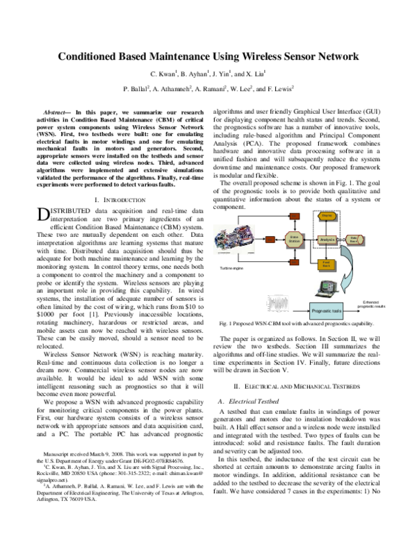The overall proposed scheme is shown in Fig. 1. The goal of the prognostic tools is to provide both qualitative and quantitative information about the status of a system or component. SN SN Base Base Station Station SN Turbine engine Display Display Analysis Analysis Data Data Base Base Feed Feed Back Back Enhanced prognostic results Prognostic tools Fig. 1 Proposed WSN-CBM tool with advanced prognostics capability. The paper is organized as follows. In Section II, we will review the two testbeds. Section III summarizes the algorithms and off-line studies. We will summarize the realtime experiments in Section IV. Finally, future directions will be drawn in Section V. II. ELECTRICAL AND MECHANICAL TESTBEDS A. Electrical Testbed A testbed that can emulate faults in windings of power generators and motors due to insulation breakdown was built. A Hall effect sensor and a wireless node were installed and integrated with the testbed. Two types of faults can be introduced: solid and resistance faults. The fault duration and severity can be adjusted too. In this testbed, the inductance of the test circuit can be shorted at certain amounts to demonstrate arcing faults in motor windings. In addition, additional resistance can be added to the testbed to decrease the severity of the electrical fault. We have considered 7 cases in the experiments: 1) No inductance shortage (Baseline); 2) 10 mH shorted; 3) 20 mH shorted; 4) 30 mH shorted; 5) 10 mH shorted with the addition of 10 ohms; 6) 20 mH shorted with the addition of 10 ohms; 7) 30 mH shorted with the addition of 10 ohms. The sampling rate of the data collection is 1.2 kHz. For 6 consecutive days, 5 sets of data were collected for each of the 7 cases. To simulate the stator coil of a motor or a generator, different sizes of inductors (a mH, b mH, and so on) are connected in series. Fig. 2 shows the conceptual design of the test-bed for electrical faults. The inductance values are: 1, 2.5, 5, 10, 20 and 30 mH. They can be rearranged within the series combination of the whole coil (L coil = 68.5 mH) to apply the fault on the following different inductance values: 1 2.5 3.5 5 6 7.5 8.5 10 11 12.5 Fig. 4 Finished testbed. We used the Microstrain wireless accelerometer node where a triaxial accelerometer is combined with data logging transceiver for use in high speed wireless sensor networks. Fig. 5 shows the wireless sensor node for vibration data collection. Inductance Coils a mH b mH c mH d mH e mH f mH g mH Fuse WSN Hall Effect Sensor Variable Resistor Fault Generator Switch Power Source Fig. 2 Conceptual design of the test-bed for electrical faults. Data is collected using a Hall Effect Sensor (Fig. 3). This sensor is interfaced to a Crossbow Mica2 mote (Fig. 3) for RF transmission. Fig. 5 Wireless accelerometer node. The range is more than 70 meters. III. REAL-TIME ALGORITHMS AND OFF-LINE STUDIES Board for interfacing Hall Effect sensor Mica2 mote Fig. 3 Left: Hall effect sensor; Right: Wireless mote. B. Mechanical Testbed There are critical rotating components such as bearing and gearbox in generators and motors. Ensuring healthy conditions of these components will reduce system downtime and save maintenance costs. We set up a testbed to demonstrate mechanical faults where accelerometers are used for vibration sensing through the means of wireless data collection. The testbed consists of a flywheel that is attached to a shaft rotated by an electrical motor. Fig. 4 shows the finished testbed. A. Wireless Data Correction It was observed from some of the collected wireless raw data that there were discrepancies in the raw data waveform (see Fig. 6-a). Although these discrepancies were localized in limited sections of the data waveform, they still have caused considerable effects on the spectrum of the data (see Fig. 6-c). In order to reduce these unwanted effects, a data correction algorithm has been developed. The algorithm corrected these discrepancies and resulted in correct spectrum waveforms (see Fig. 6-b,c). noticed that the amplitude difference of the peaks differ for the two classes. The new feature takes advantage of this difference. The new feature is basically the ratio of the “baseline peak” to the “maximum peak”. For introduction of these terms, see Fig. 7. 125 120 115 Amplitude 110 Solid - 10mH (beg20mh1) 105 Max peak 150 100 140 95 Baseline peak 130 90 120 85 110 80 7080 7100 7120 7140 No 7160 7180 7200 100 90 a) Wireless raw data 80 125 70 120 60 115 50 4000 6000 8000 10000 12000 14000 16000 18000 Fig. 7 Introduction of max and baseline peaks. The new feature is applied to 6 days data. The values of the new feature are shown in Fig. 8. It is seen that for five classes, thresholds can be assigned where 5 of 7 classes can be distinguished from each other. These thresholds are shown as dotted lines in Fig. 8. On the other hand for Faultless and Res10-10mH classes, an overlapping between their samples is observed. Thus, for values upper than 0.897 (new feature value), there is a need for another measure to differentiate between these two overlapping classes. Based on some additional analysis, another rule was developed to differentiate the faultless and the Res10-10mH cases. 90 85 80 6950 7000 7050 No 7100 7150 7200 b) Wireless data (After correction) 4 10 Raw data After correction 2 10 1 0 10 Amplitude 2000 100 95 -2 10 -4 10 -6 10 0 105 0 100 200 300 Frequency (Hz) 400 500 600 c) Spectrums before and after correction Fig. 6 Discrepancy in wireless data and the spectrums before and after correction B. Electrical Fault Classification Algorithms We applied two methods to classify the several fault cases. One is based on Spectral Angle Mapper (SAM) [2] and the other one is a rule-based algorithm. SAM approach has reasonable performance. However, it has been seen that due to similarity in waveform shapes of the reference signatures, SAM method has misclassification errors. Thus, instead of the spectrum signature, a new feature has been considered. When the time domain plots of the close reference signature classes are considered (see Fig. 7), it is Baseline Peak/Max Peak (normalized between 0 and 1) Amplitude 110 Faultless Solid-10mH Solid-20mH Solid-30mH Res10-10mH Res10-20mH Res10-30mH 0.897 0.9 0.82 0.8 0.72 0.7 0.618 0.6 0.5 0.45 0.4 0 0.2 0.4 0.6 0.8 1 1.2 1.4 1.6 1.8 2 Fig. 8 Ratio of the “baseline peak” to the “maximum peak” values for the 6 days data The rule-based approach is applied to the 6 days data and the resultant confusion matrix is shown in Table 1. It can be seen from Table 1 that with the selected thresholds in the identified rules, the classification results are almost perfect with only 1 miss out of 30 in Faultless class data. Table 1 Confusion matrix for rule based-approach (Testing data set consist of 6 days measurements) Faultless 96.67 0.00 0.00 0.00 0.00 0.00 0.00 Faultless Solid-10mH Solid-20mH Solid-30mH 10ohm-10mH 10ohm-20mH 10ohm-30mH Solid-10mH 0.00 100.00 0.00 0.00 0.00 0.00 0.00 Solid-20mH 0.00 0.00 100.00 0.00 0.00 0.00 0.00 Solid-30mH 0.00 0.00 0.00 100.00 0.00 0.00 0.00 10ohm-10mH 0.00 0.00 0.00 0.00 100.00 0.00 0.00 10ohm-20mH 3.33 0.00 0.00 0.00 0.00 100.00 0.00 10ohm-30mH 0.00 0.00 0.00 0.00 0.00 0.00 100.00 C. Mechanical Fault Health Trending We developed a proprietary health trending algorithm based on PCA [3]. In the training part, only the normal data have been used to compute the principal components which will form the PCA model. In the testing part, the test data of interest is projected to the principal components after being subtracted from the mean. In Fig. 9, the x-axis is used to represent the “data measurement no”. The following index table shows what these measurements correspond to. It can be observed from the health index values that the index value increases as the mass of the weight is increased or the mass is put to a further outside location in the flywheel. Among the three channels, the X channel seems to yield index values with less variation when compared to other 2 channels or the concatenation of 3 channels. Index ------1:25 26:50 51:75 76:100 101:125 126:150 151:175 176:200 201:225 226:250 251:275 276:300 301:325 Information ------------------Day1,2,3,4,5, No load measurements, 5 for each day Day1,2,3,4,5, 5grams Inner location measurements, Day1,2,3,4,5, 5grams Middle location measurements, Day1,2,3,4,5, 5grams Outer location measurements, Day1,2,3,4,5, 10grams Inner location measurements, Day1,2,3,4,5, 10grams Middle location measurements, Day1,2,3,4,5, 10grams Outer location measurements, Day1,2,3,4,5, 15grams Inner location measurements, Day1,2,3,4,5, 15grams Middle location measurements, Day1,2,3,4,5, 15grams Outer location measurements, Day1,2,3,4,5, 20grams Inner location measurements, Day1,2,3,4,5, 20grams Middle location measurements, Day1,2,3,4,5, 20grams Outer location measurements, Channel 2 (X) 0.8 0.7 PCA health index A. Real-time Fault Diagnostic System for Motor/Generator Winding Faults The first prototype is for detecting faults and estimating fault sizes in the electrical testbed, which emulates insulation problems in windings of motors and generators. The algorithms have been described in Section II. There are several modules in our prototype: 1) Input module for acquiring data; 2) Wireless data correction module; 3) Processing module for fault classification; 4) Output module for displaying decisions. The GUI of this prototype is shown in Fig. 10. Fig. 10 Fault diagnostic prototype for motor/generator winding fault classification. There are 3 fault cases: no fault, solid fault, and resistance fault. Within the solid fault case, we have 3 situations: 10 mH, 20 mH, and 30 mH. For the resistance faults, we also have 3 cases: 10 ohm and 10 mH, 10 ohm and 20 mH, and 10 ohm and 30 mH. The different cases have different spectral shapes and hence can be differentiated. Real-time experiments were performed. We have run experiments for each case. Video clips were recorded. Here we include a few snap shots of 3 representative cases. • No fault The experiment was recorded by using a camcorder. Fig. 11 (a) shows the time domain data from the wireless sensor and (b) shows the real-time classification results of our tool. It can be seen that “no fault” condition was correctly classified. 0.6 0.5 0.4 0.3 0.2 0.1 0 IV. REAL-TIME PROTOTYPES AND EXPERIMENTS 0 50 100 150 200 Measurement no 250 300 350 Fig. 9 PCA Health index values using Channel 2 (X) for 5 days measurements (3 locations, no load and 4 weights), number of principal components: 15 (a) (c) Real-time classification results. Fig. 12 (a) 30 mH inductor; (b) Scope shows sensor data; (c) Decision of the our real-time classification algorithm. • Resistance fault (10 ohm and 20 mH) This experiment is about the detection of a resistance fault. A 10 ohm resistor and 20 mH inductor were used in the experiment to emulate the fault. Fig. 13 shows the snap shots from a video clip. (d) indicates correct classification result of the experiment . (b) Fig. 11 (a) Scope shows clean sensor data; (b) Decision of our real-time classification algorithm. • Solid fault (30 mH) Fig. 12 shows the 30mH inductor used in the experiment, the oscilloscope display of the wireless sensor data, and the final decision of our real-time tool. A video clip was recorded and the images are taken from that clip. (a) Adjustable resistor (b) 20 mH inductor (a) 30 mH inductor (c) Motor coil emulator (b) Sensor output (d) Classification result Fig. 13 Real-time classification of a resistance fault. B. Real-time Fault Diagnostic System for Mechanical Faults Similar to the first prototype, the second prototype consists of the following modules: 1) Input module for acquiring accelerometer data; 2) PCA health monitoring tool; 3) Output module for displaying health index. The basic idea in PCA is to use the fault free data to get a system model. If the system health deviates from the normal status, the health index will increase. The higher the vibration level, the larger the health index will be. The GUI for this prototype is shown in Fig. 14. Fig. 15 Real-time detection of a 5 gram off-balance. • 15 gram outer ring Here a 15 gram screw was attached to the outer ring of the flywheel. The figure below shows a snap shot of the video. Now the vibration level was quite large as compared to the 5 gram case. Fig. 16 Real-time detection of a 15 gram off-balance. V. FUTURE DIRECTIONS We are currently trying to commercialize our real-time systems to some potential users. Our goal is to embed our system into motors and generators. Fig. 14 Fault diagnostic prototype for mechanical fault classification. VI. ACKNOWLEGEMENT Many real-time experiments were performed. We include two cases. • 5 gram in the middle of the flywheel A 5 gram screw was added to the middle of the flywheel. The vibration data were collected and wirelessly transmitted to a receiver near the processing center. The figure below shows a snapshot of the video. It can be seen the vibration level was not very large. A health index was produced by our tool. The authors would like to thank Ms. Jenny Tennant for proofreading our paper and providing valuable comments. REFERENCES [1] [2] [3] A. Tiwari, P. Ballal, F. L. Lewis, “Energy-Efficient Wireless Sensor Network Design & Implementation for Condition Based Maintenance,” ACM Trans. On Sensor Network. 2007. C.-I. Chang, Hyperspectral Imaging: Techniques for Spectral Detection and Classification, Springer, 2003. S. Haykin, Neural Network: A Comprehensive Foundation, PrenticeHall, 1998.