SIAM J. COMPUT.
Vol. 48, No. 5, pp. 1603–1642
c 2019 Society for Industrial and Applied Mathematics
\bigcirc
BICRITERIA DATA COMPRESSION\ast
ANDREA FARRUGGIA† , PAOLO FERRAGINA† , ANTONIO FRANGIONI† , AND
ROSSANO VENTURINI†
Abstract. Since the seminal work by Shannon, theoreticians have focused on designing compressors targeted at minimizing the output size without sacrificing much of the compression/decompression
efficiency. On the other hand, software engineers have deployed several heuristics to implement compressors aimed at trading compressed space versus compression/decompression efficiency in order
to match their application needs. In this paper we fill this gap by introducing the bicriteria datacompression problem that seeks to determine the shortest compressed file that can be decompressed
in a given time bound. Then, inspired by modern data-storage applications, we instantiate the
problem onto the family of Lempel–Ziv-based compressors (such as Snappy and LZ4) and solve it
by combining in a novel and efficient way optimization techniques, string-matching data structures,
and shortest path algorithms over properly (bi-)weighted graphs derived from the data-compression
problem at hand. An extensive set of experiments complements our theoretical achievements by
showing that the proposed algorithmic solution is very competitive with respect to state-of-the-art
highly engineered compressors.
Key words. approximation algorithm, data compression, Lempel–Ziv 77, Pareto optimization
AMS subject classifications. 68P30, 90C27
DOI. 10.1137/17M1121457
1. Introduction. The advent of massive datasets and the consequent design of
high-performing distributed storage systems, such as Bigtable by Google [11], Cassandra by Facebook [7], and Hadoop by Apache, have reignited the interest of the scientific and engineering community towards the design of lossless data compressors that
achieve effective compression ratio and very high decompression speed. The literature
abounds with solutions for this problem, referred to as “compress once, decompress
many times.” These solutions can be cast into two main families: the compressors
based on the Burrows–Wheeler transform (BWT) [10], and the ones based on the
Lempel–Ziv parsing scheme [44, 45]. Algorithms are known in both families that require linear time in the input size, both for compressing and decompressing the data,
and size of the compressed file that can be bound in terms of the kth order empirical
entropy of the input [30, 44].
The compressors running behind real-world large-scale storage systems, however,
are not derived from those scientific results. The reason is that theoretically efficient
compressors are optimal in the RAM model, but they elicit many cache/IO misses on
decompression. This poor behavior is most prominent in the BWT-based compressors, and it is also not negligible in the Lempel–Ziv (LZ)-based approaches. This motivated the software engineers to devise variants of Lempel and Ziv’s original proposal
(e.g., Snappy, Lz4) with the injection of several software tricks that have beneficial
effects on memory-access locality. These compressors expanded further the known
∗ Received by the editors March 17, 2017; accepted for publication (in revised form) August 9,
2019; published electronically October 31, 2019. This paper combines and extends two conference
papers that appeared in the proceedings of the ACM-SIAM Symposium on Discrete Algorithms
(2014) and of the European Symposium on Algorithms (2014).
https://doi.org/10.1137/17M1121457
† Department of Computer Science, University of Pisa, 56123 Pisa, Italy (a.farruggia@di.unipi.it,
paolo.ferragina@unipi.it, antonio.frangioni@unipi.it, rossano.venturini@unipi.it).
1603
�1604
FARRUGGIA, FERRAGINA, FRANGIONI, AND VENTURINI
jungle of time/space trade-offs,1 thus confronting software engineers with a difficult
choice: either achieve effective/optimal compression ratios, at the possible sacrifice of
decompression speed (as occurs in the known theory-based results [18, 19, 20]), or try
to balance compression ratio versus decompression speed by adopting a plethora of
programming tricks that actually waive any mathematical guarantees on their final
performance (such as in Snappy, Lz4) or by adopting approaches that can only offer a
rough asymptotic guarantee (such as in LZ-end, designed by Kreft and Navarro [31],
which is more suited for highly compressible datasets).
In light of this dichotomy, it would be natural to ask for an algorithm that guarantees effective compression ratio and efficient decompression speed in hierarchical
memories. In this paper, however, we aim for a more ambitious goal that is further
motivated by the following two simple, yet challenging, questions:
1. Is it possible to obtain a slightly larger compressed file than the one achievable
with BWT-based compressors while significantly improving on BWT’s decompression time? This is a natural question arising in the context of distributed
storage systems, such as the ones leading to the design of Snappy and Lz4.
2. Is it possible to obtain a compressed file that can be decompressed slightly
slower than Snappy or Lz4 while significantly improving on their compressed
space? This is a natural question in contexts where space occupancy is a major
concern, e.g., tablets and mobile phones, and for which tools like Google’s Brotli
have been recently introduced.
By providing appropriate mathematical definitions for the two fuzzy expressions
above—i.e., “slightly larger” and “slightly slower”—these two questions become pertinent and challenging in theory too. To this aim, we introduce the bicriteria data
compression problem (BDCP): given an input file \scrS and an upper bound \scrT on its
decompression time, determine a compressed version of \scrS that minimizes the compressed space provided that it can be decompressed in \scrT time. Symmetrically, we
can exchange the role of time/space resources, and thus ask for the compressed version of \scrS that minimizes the decompression time provided that the compressed space
occupancy is within a fixed bound. Of course, in order to attack this problem in a
principled way, we need to fix two ingredients: the class of compressed versions of \scrS
over which the bicriteria optimization will take place, and the computational model
measuring the resources to be optimized.
For the former ingredient we select the class of LZ77-based compressors, which
are dominant both in the theoretical setting (e.g., [12, 13, 17, 20, 26, 27]) and in the
practical setting (e.g., Gzip, 7zip, Snappy, Lz4 [29, 31, 43]). In section 2 we show
that BDCP formulated over LZ77-based compressors is a theoretically sound problem
because there exists an infinite class of strings that can be parsed in many different
ways and can offer a wide spectrum of time/space trade-offs in which small variations
in the usage of one resource (e.g., time) may induce arbitrarily large variations in the
usage of the other resource (e.g., space).
For the latter ingredient we take inspiration from several known models of computation that abstract multilevel memory hierarchies and the fetching of contiguous
memory words (Aggarwal and colleagues [1, 2], Alpern et al. [5], Luccio and Pagli [35],
and Vitter and Shriver [42]). In these models the cost of fetching a word at address
x takes f (x) time, where f (x) is a nondecreasing, polynomially bounded function
(e.g., f (x) = \lceil log x\rceil and f (x) = xΘ(1) ). Some of these models offer also a block-copy
operation, in which a sequence of \ell consecutive words can be copied from memory
1 See,
e.g., http://mattmahoney.net/dc/.
�BICRITERIA DATA COMPRESSION
1605
location x to memory location y (with x \geq y) in time f (x) + \ell . We remark that, in
our scenario, this model is more proper than the frequently adopted two-level memory
model [4], because we care to differentiate between contiguous and random accesses
to memory/disk blocks, this being a feature heavily exploited in the implementation
of modern compressors [14].
Given these two ingredients, we devise a formal framework that allows us to
analyze any LZ77-parsing scheme in terms of both the space occupancy (in bits) of
the compressed file, and the time cost of its decompression, taking into account the
underlying memory hierarchy. More specifically, we start from the model proposed
by Ferragina, Nitto, and Venturini [20] that represents the input text \scrS via a special
weighted directed \bigl( acyclic
\bigr) graph (DAG) consisting of n = | \scrS | nodes, one per character
of \scrS , and m = \scrO n2 edges, one per possible phrase in the LZ77-parsing of \scrS . We
augment this graph by labeling each edge with two costs: a time cost, which accounts
for the time to decompress an LZ77-phrase (derived according to the hierarchicalmemory model mentioned above), and a space cost, which accounts for the number
of bits needed to store the LZ77-phrase associated to that edge (derived according to
the integer encoder adopted in the compressor). Every path \pi from node 1 to node n
in \scrG (hereafter, “1n-path”) corresponds to an LZ77-parsing of the input file \scrS , whose
compressed-space occupancy is given by the sum of the space costs of \pi ’s edges (say,
s(\pi )) and whose decompression time is given by the sum of the time costs of \pi ’s edges
(say, t(\pi )). As a result, we are able to reformulate BDCP as a weight-constrained
shortest path problem (WCSPP) over the weighted DAG \scrG , seeking for the 1n-path \pi
that minimizes the compressed-space occupancy s(\pi ) among all those 1n-paths whose
decompression time is t(\pi ) \leq \scrT .
Due to its vast range of applications WCSPP received a great deal of attention from
the optimization community; see, e.g., the work by Mehlhorn and Ziegelmann [38] and
references therein. It is an \scrN \scrP -hard problem, even when the DAG \scrG has positive costs
[15, 21], but not strongly \scrN \scrP -hard as it can be solved in pseudopolynomial \scrO (m\scrT )
time via dynamic programming [33]. Our version of the WCSPP problem has the
parameters m and \scrT bounded
\bigl( by \scrO (n\bigr) log n) (see
\bigl( section
\bigr) 2), so it can be solved in
polynomial time \scrO (m\scrT ) = \scrO n2 log2 n and \scrO n2 log n space. Unfortunately these
bounds are unacceptable in practice, because n2 \approx 264 just for one gigabyte of data
to be compressed.
The first algorithmic contribution of this paper is to exploit the structural properties of the weighted DAG in order
to design
an algorithm that approximately solves
\bigl(
\bigr)
the corresponding WCSPP in \scrO n log2 n time and \scrO (n) working space. The approximation is additive, that is, our algorithm determines an LZ77-parsing of \scrS whose
decompression time is \leq \scrT + 2 tmax and whose compressed space is just at most smax
bits more than the optimal one, where tmax and smax are, respectively, the maximum time cost and the maximum space cost of any edge in the DAG. Notably, the
values of smax and tmax are logarithmic in n so those additive terms are negligible
(see section 2). We remark here that this type of additive approximation is clearly
related to the bicriteria-approximation introduced by Marathe et al. [36], and it is
more desirable than the “classic” (\alpha , \beta )-approximation [34], which is multiplicative.
A further peculiarity of our solution is that the additive approximation is used to
2
speed up the solution from
\bigl( Ω(n
\bigr) ) time, which is poly-time but unusable in practice,
2
to the more practical \scrO n log n time. In section 4.4 we show that our solution can
be easily generalized over graphs satisfying some simple properties, which might be
of independent interest.
The bicriteria strategy proposed in this paper deploys as a subroutine the bit-
�1606
FARRUGGIA, FERRAGINA, FRANGIONI, AND VENTURINI
optimal LZ77-compressor devised by Ferragina, Nitto, and Venturini [20]. Unfortunately that algorithm, albeit asymptotically optimal in the RAM model, is not efficient
in practice due to its expensive pattern of memory accesses. As a second algorithmic
contribution, we propose a novel asymptotically optimal LZ77-compressor, hereafter
named LzOpt, that is significantly faster in practice because it exploits simpler data
structures and accesses memory in a sequential fashion (see section 3.2). This represents an important step in closing the compression-time gap between LzOpt and the
widely used compressors such as Gzip, Bzip2, and Lzma2.
As a third, and last, contribution of this paper we experimentally evaluate both
LzOpt and the resulting bicriteria compressor, hereafter named Bc-Zip, under various experimental scenarios (see section 5). We investigate many algorithmic and
implementation issues on several datasets of different types. We also compare their
performance with an ample set of both classic (LZ-based, PPM-based, and BWTbased) and engineered (Snappy, Lz4, Lzma2, and Ppmd) compressors. The whole
experimental setting originated by this effort, consisting of the datasets and the
C++ code of Bc-Zip, has been made available to the scientific community to allow the replication of those experiments and the possible testing of new solutions
(see https://github.com/farruggia/bc-zip). Eventually, the experiments reveal two
key aspects:
1. The two questions posed at the beginning of the paper are indeed pertinent,
because real texts can be parsed in many different ways, offering a wide spectrum
of time/space trade-offs in which small variations in the usage of one resource
(e.g., time) may induce arbitrary large variations in the usage of the other
resource (e.g., space). This motivates the introduction of our novel parsing
strategy.
2. Our parsing strategy actually dominates all the highly engineered competitors,
by exhibiting decompression speeds close to or better than those achieved by
Snappy and Lz4 (i.e., the fastest ones) and compression ratios close to those
achieved by BWT-based and Lzma2 compressors (i.e., the more succinct ones).
The paper is organized as follows. In section 2 we briefly introduce the LZ77 parsing scheme, we define the models for estimating the compressed space (section 2.1) and
decompression time (section 2.2) of a given parsing, and we show an infinite family of
strings that exhibit many different time/space trade-offs (section 2.3). In section 3 we
illustrate the bit-optimal parsing introduced by Ferragina, Nitto, and Venturini [20].
In particular, in section 3.1 we briefly review their work, while in section 3.2 we illustrate our algorithmic improvements aimed at making the approach more efficient
and practical. In section 4 we illustrate our novel bicriteria strategy and obtain the
approximation result. Section 5 details our experiments and some interesting implementation choices: section 5.1 illustrates how to extend the bit-optimal and bicriteria
strategies to take into account literals strings, i.e., LZ77-phrases that represent an
uncompressed sequence of characters, while section 5.2 illustrates the performance of
the new bit-optimal parser illustrated in section 3.2. Section 5.3 integrates section 2.2
with additional details about deriving a time model in an automated fashion on an
actual machine, as well as showing its accuracy on our experimental setting. Section 5.4 illustrates the performance of the bicriteria parser on our dataset. Finally, in
section 6 we sum up this work and point out some interesting future research on the
subject.
2. On the LZ77-parsing. Let \scrS be a string of length n built over an alphabet
Σ = [\sigma ] and terminated by a special character. We denote by \scrS [i] the ith character
�BICRITERIA DATA COMPRESSION
1607
of \scrS and by \scrS [i, j] the substring ranging from position i to position j (included).
The compression algorithm LZ77 works by parsing the input string \scrS into phrases
p1 , . . . , pk such that phrase pi can be either a single character or a substring that
occurs also in the prefix p1 \cdot \cdot \cdot pi - 1 , and thus can be copied from there. Once the
parsing has been identified, each phrase is represented via pairs of integers \langle d, \ell \rangle ,
where d is the distance from the (previous) position where the copied phrase occurs,
and \ell is its length. Every first occurrence of a new character c is encoded as \langle 0, c\rangle .
These pairs are compressed into codewords via variable-length integer encoders that
eventually produce the compressed output of \scrS as a sequence of bits. Among all
possible parsing strategies, the greedy parsing is widely adopted: it chooses pi as the
longest prefix of the remaining suffix of \scrS . This is optimal whenever the goal is to
minimize the number of generated phrases or, equivalently, the size of the compressed
file under the assumption that these phrases are encoded with the same number of
bits; however, if phrases are encoded with a variable number of bits, then the greedy
approach may be highly suboptimal [20], and this justifies the study and results
introduced in this paper.
2.1. Modeling space occupancy. An LZ77-phrase \langle d, \ell \rangle is typically compressed
by using two distinct (universal) integer encoders encdist and enclen , since distances
d and lengths \ell have different distributions in \scrS . We use s(d, \ell ) to denote the length
in bits of the encoding of \langle d, \ell \rangle , that is, s(d, \ell ) = | encdist (d)| + | enclen (\ell )| . We assume
that a phrase consisting of one single character is represented by a fixed number of
bits. We restrict our attention to variable-length integer encoders that emit longer
codewords for bigger integers. This property is called the nondecreasing cost property
and is stated as follows.
Property 2.1. An integer encoder enc satisfies the nondecreasing cost property
if | enc(n)| \leq | enc(n\prime )| for all positive integers n \leq n\prime .
We also assume that these encoders must be stateless, that is, they must always
encode the same integer with the same bit sequence. These two assumptions are not
restrictive because they encompass all known universal encoders, such as truncated
binary, Elias’ Gamma and Delta [16, 22], and Lz4’s encoder.2
In the following
(see Table 2.1 for a recap of the main notation), we denote
\sum
by s(\scrP ) =
\langle d,\ell \rangle \in \scrP s(d, \ell ) the length in bits of the compressed output generated
according to the LZ77-parsing \scrP . We also denote by scosts the number of distinct
values assumed by s(d, \ell ) when d, \ell \leq n; this value is relevant as it affects the time
complexity of the parsing strategies presented in this paper. Further, we denote as
Qdist the number of times the value | encdist (d)| changes when d = 1, . . . , n; value Qlen
is defined in a similar way. Under the assumption that both encdist and enclen satisfy
Property 2.1, it holds that scosts = Qdist + Qlen . Most interesting integer encoders,
such as those listed above, encode integers in a number of bits proportional to their
logarithm, and, thus, both Qdist and Qlen are \scrO (log n).
2.2. Modeling decompression time. The aim of this section is to define a
model that can accurately predict the decompression time of an LZ77-compressed
text in modern machines, characterized by memory hierarchies equipped with cache2 We notice that other well-known integer encoders that do not satisfy the nondecreasing cost
property, such as PForDelta and Simple9, are indeed not universal and, crucially, are designed to
be effective only in some specific situations, such as the encoding of inverted lists. Since these
settings have very specific assumptions about symbol distribution that are generally not satisfied by
LZ77-parsings, they are not examined in this paper.
�1608
FARRUGGIA, FERRAGINA, FRANGIONI, AND VENTURINI
Table 2.1
Summary of main notation.
Name
Definition
\scrS
n
\scrS [i]
\scrS [i, j]
A (null-terminated) document to be compressed.
Length of \scrS (end-of-text character included).
The ith character of \scrS .
Substring of \scrS starting from \scrS [i] until \scrS [j] (included).
\langle d, \ell \rangle
\langle 0, c\rangle
\langle \ell , \alpha \rangle L
An LZ77-phrase of length \ell that can be copied at distance d.
An LZ77-phrase that represents the single character c.
An LZ77-phrase that represents a substring \alpha of length \ell .
t(d)
s(d, \ell )
Amount of time spent in accessing the first character of a copy at distance d.
The length in bits of the encoding of \langle d, \ell \rangle .
t(d, \ell )
The time needed to decompress the LZ77-phrase \langle d, \ell \rangle .
s(\pi )
t(\pi )
smax
tmax
The
The
The
The
scosts
tcosts
Q
L(k)
M (k)
E(k)
The number of distinct values that may be assumed by s(d, \ell ) when d \leq n, \ell \leq n.
The number of distinct values that may be assumed by t(d, \ell ) when d \leq n, \ell \leq n.
Number of cost classes for the integer encoder enc (may depend on n).
Codeword length (in bits) of integers belonging to the kth cost class of enc.
Largest integer encodable by the kth cost class of enc.
Number of integers encodable within the kth cost class (i.e., E(k) = M (k) -
M (k - 1)).
Defined as the jth block of E(k) contiguous nodes in the graph \scrG .
W (k, j)
Sa[1, n]
Isa[1, n]
space occupancy of parsing \pi .
time needed to decompress the parsing \pi .
maximum space occupancy (in bits) of any LZ77-phrase of \scrS .
maximum time taken to decompress a LZ77-phrase of \scrS .
The suffix array of \scrS ; hence Sa[i] is the ith lexicographically smallest suffix of \scrS .
The inverse suffix array, so Isa[j] is the (lexicographic) position of \scrS [j, n] among
all text suffixes, hence in Sa (i.e., j = Sa[Isa[j]]).
prefetching strategies and sophisticated control-flow predictive processors. In a fashion analogous to the previous section, we assume that decoding a character \langle 0, c\rangle
takes constant time t\scrC , while function t(d, \ell ) models the time spent in decoding an
LZ77-phrase \langle d, \ell \rangle and performing the phrase copy. The time\sum
needed to decompress
parsing \scrP (and so reconstruct \scrS ) is thus estimated as t(\scrP ) = \langle d,\ell \rangle \in \scrP t(d, \ell ).
Modeling the time spent in decoding an LZ77-phrase \langle d, \ell \rangle , denoted as t\scrD (d, \ell ),
is easy, as it is either constant or proportional to s(d, \ell ). On the other hand, modeling the time spent in copying is trickier, as it needs to take into account memory
hierarchies. To do this, we take inspiration from several known hierarchical-memory
models (Aggarwal and colleagues [1, 2], Alpern et al. [5], Luccio and Pagli [35], and
Vitter and Shriver [42]). Let t(d) be the access latency of the fastest (smallest) memory level that can hold at least d characters: we assume that accessing a character at
distance d takes time t(d). However, the time spent in copying \ell characters going back
d positions in \scrS is highly influenced by prefetching and the way memory is laid out.
Indeed, memory hierarchies in modern machines consist of multiple levels of memory
(“caches”), where each cache-level Ci logically partitions the memory address space
into cache-lines of size Li . When an address x is requested to a cache of level i,
the whole cache-line containing address x is transferred; hence, reading \ell characters
from cache Ci needs only \lceil \ell /Li \rceil accesses to cache Ci . Moreover, cache-prefetching is
typically used to lower even further the time needed to read chunks of memory. In
fact, when a sequence of cache misses to contiguous cache lines is triggered by the
�BICRITERIA DATA COMPRESSION
1609
processor, it instructs the cache to “stream” adjacent lines without an explicit processor request. After prefetching takes place, accessing subsequent characters from
the cache Ci has the same cost as reading them from the closest (fastest) cache. The
number of cache misses needed to trigger prefetching is hardware specific and difficult
to estimate in advance, but it is usually two [14]. The cost of reading \ell contiguous
characters from a given memory level Ci is thus the cost of reading \ell characters from
the fastest memory level plus at most two cache misses in Ci , which we estimate with
the term nM (\ell ) \leq 2.
Summing up, processing a phrase \langle d, \ell \rangle takes time
\Biggl\{
t\scrD (d, \ell ) + nM (\ell ) t(d) + \ell t\scrC if \ell > 0,
t(d, \ell ) =
t\scrC
if \ell = 0.
Let us now estimate tcosts , the number of times t(d, \ell ) changes when d, \ell \leq n.
Analogously to scosts , this term affects the time complexity of the parsing strategies
proposed in this paper, and therefore it is desirable that it is as low as possible.
Since t(d, \ell ) has an additive term \ell t\scrC , tcosts is \scrO (n). However, the overall contribution of this term to t(\scrP ) is always n t\scrC , so it can be taken into account by removing
it from the definition of t(d, \ell ) and by setting the time bound as \scrT - n t\scrC . As previously
remarked, the term t\scrD (d, \ell ) is proportional to the codeword length s(d, \ell ); hence, by
definition, it changes scosts times when d, \ell \leq n. Furthermore it is nM (\ell ) \leq 2 and
t(d) = \scrO (log n) because sizes in hierarchical memories grow exponentially. Thus it
follows that tcosts = \scrO (scosts + log n).
Further details on the actual evaluation of the various parameters, as well as its
actual decompression-time accuracy, are given in section 5.3.
2.3. Pathological strings: Trade-offs in space and time. We are interested
in a parsing strategy that optimizes two different criteria, namely decompression time
and compressed space. Unfortunately, usually there is no parsing that optimizes both
of them, but, instead, there are several parsings that offer distinct time/space tradeoffs. We thus have to turn our attention to Pareto-optimal parsings, i.e., parsings that
are not dominated by any other parsing by being strictly worse on one account and
not better on the other. We now show that there exists an infinite family of strings
whose Pareto-optimal parsings exhibit significant differences in their decompression
time versus compressed space.
Let us assume, for simplicity’s sake, that each codeword takes constant space;
moreover, let us also assume that memory is arranged in just two levels: a fastest
level (of size c) with negligible access time and a slowest level (of unbounded size)
with substantial access time. We construct our pathological input string \scrS as follows.
Let Σ = Σ\prime \cup $, with $ a character not in Σ\prime , and let P be a string of length at most
c, drawn over Σ\prime , whose greedy LZ77-parsing takes k phrases. For any i \geq 0, let Bi
be the string $c+i P . Set \scrS = B0 B1 . . . Bm . Since the length of run of $s increases as i
increases, and since character $ does not occur in P , no pair of consecutive strings Bi
and Bi+1 can be part of the same LZ77-phrase. Moreover, we have two alternatives in
parsing each Bi , with i \geq 1: either (i) we copy everything inside Bi , a strategy that
takes 2 + k phrases of distance at most c and no cache miss at decompression time, or
(ii) we copy from the previous string Bi - 1 , taking two phrases (a copy and a single
character $) and one cache miss at decompression time. There are m Pareto-optimal
parsings of \scrS obtained by choosing either the first or the second of the two alternatives
just outlined for each string Bi\geq 1 : given a positive number m
\widetilde \leq m of cache misses,
the parsing that only copies blocks Bm - m+1
, . . . , Bm has a smaller compressed space
\widetilde
�1610
FARRUGGIA, FERRAGINA, FRANGIONI, AND VENTURINI
than any other parsing with the same number m
\widetilde of cache misses. At one extreme,
the parser always chooses alternative (i), thus obtaining a parsing with m(2 + k)
phrases that is decompressible with no cache misses. At the other extreme, the parser
always prefers alternative (ii), thus obtaining a parsing with 2 + k + 2m phrases that
is decompressible with m cache misses (notice that block B0 cannot be copied). A
whole range of Pareto-optimal parsings stands between these two extremes, allowing
us to trade decompression speed for space occupancy. In particular, one can save k
phrases at the cost of one more cache miss, where k is a value that can be varied by
choosing different strings P . The bicriteria strategy, illustrated in section 4, allows us
to efficiently choose any of these trade-offs.
3. On the bit-optimal compression. In this section we discuss the bit-optimal
LZ77-parsing problem (BLPP), defined as follows: given a text \scrS and two integer
encoders encdist and enclen , determine the minimal-space LZ77-parsing of \scrS provided
that all phrases are encoded with encdist (for the distance component) and enclen
(for the length component). Ferragina, Nitto, and Venturini [20] have shown an
(asymptotically) efficient algorithm for this problem, proving the following theorem.
Theorem 3.1. Given a string \scrS and two integer-encoding functions encdist and
enclen that satisfy Property 2.1, there exists an algorithm to compute the bit-optimal
LZ77-parsing of \scrS in \scrO (n \cdot scosts ) time and \scrO (n) words of space.
In this section we illustrate a novel BLPP algorithm that is much simpler, and
therefore more efficient in practice, while still achieving the same time/space asymptotic complexities stated in the theorem above. Since BLPP is a key step for solving
the bicriteria data compression problem (BDCP), these improvements are crucial to
obtain an efficient bicriteria parser as well.
Our new algorithm relies on the same optimization framework devised by Ferragina, Nitto, and Venturini [20]. For the sake of clarity, we illustrate that framework in
section 3.1, restating some lemmas and theorems proved in that paper. Briefly, the
authors show how to reduce the BLPP to a shortest path problem on a DAG \scrG with
one node per character and one edge for every LZ77-phrase. However, even though
the shortest path problem on DAGs can be solved linearly in the size of the graph,
\bigl( \bigr)
a straight resolution of BLPP would be inefficient because \scrG might consist of \scrO n2
edges. The authors solve this problem in two steps: first, \scrG is pruned to a graph
\scrG \widetilde with just \scrO (n \cdot scosts ) edges, still retaining at least one optimal solution; second,
the graph \scrG \widetilde is generated on-the-fly in constant amortized time per edge, so that the
shortest path can be computed in the time and space bounds stated in Theorem 3.1.
We notice that the codewords generated by the most interesting universal integer encoders have logarithmic length (i.e., scosts = \scrO (log n)), so the algorithm of
Theorem 3.1 solves BLPP in \scrO (n log n) time. However, this algorithm requires the
construction of suffix arrays and compact tries of several substrings of \scrS (possibly
transformed in proper ways), which are then accessed via memory patterns that make
the algorithm pretty inefficient in practice.
In section 3.2 we show our new algorithm for the second step above, which is where
our novel solution differs from the known one [20]. Our algorithm only performs scans
over a few lists, so it is much simpler and therefore much more efficient in practice
while simultaneously achieving the same time/space asymptotic complexities stated
in Theorem 3.1.
3.1. Known results: A graph-based approach. Given an input string \scrS of
length n, BLPP is reduced to a shortest path problem over a weighted DAG \scrG that
�BICRITERIA DATA COMPRESSION
1611
consists of n + 1 nodes, one per input character plus a sink node, and m edges, one
per possible LZ77-phrase in \scrS . In particular there are two different types of edges to
consider:
(i) edge (i, i + 1), which represents the case of the single-character phrase \scrS [i], and
(ii) edge (i, j), with j = i + \ell > i + 1, which represents the substring \scrS [i, i + \ell - 1]
that also occurs previously in \scrS .
This construction is similar to the one originally proposed by Schuegraf and Heaps [41].
By definition, every path \pi in this graph is mapped to a distinct parsing \scrP , and vice
versa. An edge (i\prime , j \prime ) is said to be nested into an edge (i, j) if i \leq i\prime < j \prime \leq j. A
peculiar property of \scrG that is extensively exploited throughout this paper is that its
set of edges is closed under nesting.
Property 3.2. Given an edge (i, j) of \scrG , any edge nested in (i, j) is an edge
of \scrG .
This property follows quite easily from the prefix/suffix-complete property of the
LZ77 dictionary and from the bijection between LZ77-phrases and edges of \scrG . Since
each edge (i, j) of \scrG is associated to an LZ77-phrase, it can be weighted with the
length, in bits, of its codeword. In particular,
(i) any edge (i, i + 1), a single character \langle 0, \scrS [i]\rangle , can be assumed to have constant
cost;
(ii) for any other edge (i, j) with j > i + 1, a copy of length \ell = j - i copying
from some position i - d, is instead weighted with the value s\scrG (i, j) = s(d, \ell ) =
| enc(d)| + | enc(\ell )| , where the notation \langle d, \ell \rangle is used to denote the associated
codeword.
As it currently stands, the definition of \scrG is ambiguous whenever there exists a substring \scrS [i, j - 1] occurring more than once previously in the text: in this case, phrase
\scrS [i, j - 1] references more than one string in the LZ77 dictionary. We fix this ambiguity by selecting one phrase \langle d, \ell \rangle among those that minimize the expression s(d, \ell ).
Hence, the space cost s\scrG (\pi ) of any 1n-path \pi (from node 1 to n + 1), defined as the
sum of the costs of its edges, is the compressed size s(\scrP ) in bits of the associated
parsing \scrP . Computing the bit-optimal parsing of \scrS is thus equivalent to finding a
shortest path on the graph \scrG . In the following we drop the subscript from s\scrG whenever this does not introduce ambiguities. Since \scrG is a DAG, computing the shortest
1n-path takes \scrO (m + n) time and space; unfortunately, there are strings for which
m = Θ(n2 ) (e.g., \scrS = an generates one edge per substring of \scrS ). This means that a
naive implementation of the shortest path algorithm would not be practical even for
files of a few tens of MiBs. Two ideas have been deployed to solve this problem [20]:
1. Reduce \scrG to an asymptotically smaller subset with only \scrO (n \cdot scosts ) edges in
which the bit-optimal path is preserved.
2. Generate on-the-fly the edges in the pruned graph by means of an algorithm,
called forward star generation (FSG), that takes \scrO (1) amortized time per edge
and optimal \scrO (n) words of space. This is where our novel solution, illustrated
in section 3.2, differs.
\widetilde
Pruning the graph. We now illustrate how to construct a reduced subgraph \scrG
with only \scrO (n \cdot scosts ) edges that retains at least one optimal 1n-path of \scrG . It is easy
to show that if both encdist and enclen satisfy the nondecreasing property, then all
edges outgoing from a node have nondecreasing space costs when listed by increasing
endpoint, from left to right.
�1612
FARRUGGIA, FERRAGINA, FRANGIONI, AND VENTURINI
Lemma 3.3. If both encdist and enclen satisfy Property 2.1, then, for any node i
and for any couple of nodes j < k such that (i, j), (i, k) \in \scrG , it holds that s(i, j) \leq
s(i, k).
This monotonicity property for the space costs of \scrG ’s edges leads to the notion of
maximality of an edge.
Definition 3.4. An edge e = (i, j) is said to be maximal if and only if either the
(next) edge e\prime = (i, j + 1) does not exist, or it does exist but s(i, j) < s(i, j + 1).
Recall that scosts is the number of distinct values assumed by s(d, \ell ) for d, \ell \leq n.
By definition, every node has at most scosts maximal outgoing edges. The following
lemma shows that, for any path \pi , its “nested” paths do exist and have lower space
cost.
Lemma 3.5. For each triple of nodes i < i\prime < j, and for each path \pi from i to j,
there exists a path \pi \prime from i\prime to j such that s(\pi \prime ) \leq s(\pi ).
The lemma, used with j = n, allows us to “push” nonmaximal edges to the right
by iteratively replacing nonmaximal edges with maximal ones without augmenting
the time and space costs of the path. By exploiting this fact, Theorem 3.6 shows that
the search of shortest paths in \scrG can be limited to paths composed of maximal edges
only.
Theorem 3.6. For any 1n-path \pi there exists a 1n-path \pi \star composed of maximal
edges only and such that the space cost of \pi \star is not worse than the space cost of \pi ,
i.e., s(\pi \star ) \leq s(\pi ).
Proof. We show that any 1n-path \pi containing nonmaximal edges can be turned
into a 1n-path \pi \prime containing maximal edges only. Take the leftmost nonmaximal edge
in \pi , say (v, w), and denote by \pi v (resp., \pi w ) the prefix (resp., suffix) of path \pi ending
in v (resp., starting from w). By definition of maximality, there must exist a maximal
edge (v, z), with z > w, such that s(v, z) = s(v, w). We can apply Lemma 3.5 to the
triple (w, z, n) and thus derive a path \mu from z to n such that s(\mu ) \leq s(\pi w ). We then
construct the 1n-path \pi \prime \prime by connecting the subpath \pi v , the maximal edge (v, z), and
the path \mu : using Lemma 3.5 one readily shows that the space cost of \pi \prime \prime is not larger
than that of \pi . The key result is that we pushed right the leftmost nonmaximal edge
(if any) that must now occur (if ever) within \mu ; by iterating this argument we get the
thesis.
\widetilde obtained by keeping only maximal edges in \scrG has
Hence, the pruned graph \scrG
\scrO (n \cdot scosts ) edges. Most interesting integer encoders, such as truncated binary, Elias’
Gamma and Delta [16], Golomb [22], and Lz4’s encoder, encode integers in a number
of bits proportional to their logarithm; thus scosts = \scrO (log n) in practical settings, so
\widetilde is asymptotically sparser than \scrG , having only \scrO (n log n) edges.
\scrG
\widetilde defined by retaining only the maximal edges of
Theorem 3.7. The subgraph \scrG ,
\scrG , preserves at least one shortest 1n-path of \scrG and has \scrO (n log n) edges when using
encoders with a logarithmically growing number of cost classes.
The on-the-fly generation idea. As discussed previously, the pruning strategy
consists of retaining only the maximal edges of \scrG , that is, every edge of maximum
length among those of equal cost. Now we describe the basic ideas underlying the
generation of these maximal edges incrementally along with the shortest path computation in \scrO (1) amortized time per edge and only \scrO (n) auxiliary space. We call
this task the forward star generation (FSG). The efficient generation of the maxi-
�BICRITERIA DATA COMPRESSION
1613
mal edges needs to characterize them in a slightly different way. Let us assume,
for simplicity’s sake, that enc is used to encode both distances and lengths (that is,
enc = encdist = enclen ). If the function | enc(x)| changes only Q times when x \leq n,
then enc induces a partitioning of the range [1, n] (namely, the range of potential copydistances and copy-lengths of LZ77-phrases in \scrS ) into a sequence of Q subranges, such
that all the integers in the kth subrange are represented by enc with codewords of
length L(k) bits, with L(k) < L(k + 1). We refer to such subranges as cost classes
of enc because the integers in the same cost class are encoded by enc with the same
number of bits (hence, they have the same cost in bits). If we denote by M (k) the
largest integer in the kth cost class and set M (0) = 0, then the subrange can be
written as [M (k - 1) + 1, M (k)]. This implies that its size is E(k) = M (k) - M (k - 1),
which indeed equals the number of integers represented with exactly L(k) bits. Overall this implies that the compression of a phrase is unaffected whenever we change its
copy-distance or copy-length with integers falling in the same cost class.
Moreover, notice that an edge (i, j) associated with a phrase \langle d, \ell \rangle is maximal if it
is the longest edge taking exactly s(d, \ell ) = | enc(d)| +| enc(\ell )| bits. A maximal edge can
be either d-maximal or \ell -maximal (or both): it is d-maximal if it is the longest edge
taking exactly | enc(d)| bits for representing its distance component; \ell -maximality is
defined similarly.
Computing the d-maximal edges is the hardest task because every \ell -maximal edge
that is not also a d-maximal edge can be obtained in \scrO (1) time by “shortening” a
longer d-maximal edge. Let us illustrate this with an example: let p = (i, j) and
q = (i, k) be two consecutive d-maximal edges outgoing from vertex i with j < k, and
let \langle dp , \ell p \rangle and \langle dq , \ell q \rangle be their associated LZ77-phrases; then, all \ell -maximal edges
outgoing from vertex i whose endpoints fall between j and k have an associated phrase
of the form \langle dq , \ell \rangle , where \ell \in (\ell p , \ell q ) is an \ell cost class boundary M (v) for some cost
class v. Thus, given all d-maximal edges, generating \ell -maximal edges is as simple as
listing all \ell cost classes.
Ferragina, Nitto, and Venturini [20] employ two main ideas for the efficient computation of d-maximal edges outgoing from every node i:
1. Batch processing. The first idea allows us to bound the working space requirements to optimal \scrO (n) words. It consists of executing Q passes over the graph
\scrG , one per cost class. During the kth pass, nodes of \scrG are logically partitioned
into blocks of E(k) contiguous nodes. Each time the computation crosses a
block boundary, all the d-maximal edges spreading from that block whose copydistance can be encoded with L(k) bits are generated. These edges are kept in
memory until they are used by the shortest path algorithm, and discarded as
soon as the first node of the next block needs to be processed; the next block
of E(k) nodes is then fetched and the process repeats. Actually, all Q passes
are executed in parallel to guarantee that all d-maximal edges of a node are
available to the shortest path computation.
2. Output-sensitive d-maximal generation. The second idea allows us to compute,
for each cost class k, the d-maximal edges taking L(k) bits of a block of E(k)
contiguous nodes in \scrO (E(k)) time and space. As a result, the working space
\sum Q
complexity at any instant
is k=1 E(k)
\Bigr) = n, whereas the time complexity over
\Bigl(
\sum Q
n
all Q passes is k=1 E(k) \scrO (E(k)) = \scrO (n \cdot Q), that is, \scrO (1) amortized time
per d-maximal edge.
Let us now describe how to perform batch processing, that is, how to compute all dmaximal edges whose copy-distance can be encoded in L(k) bits and which spur from
�1614
FARRUGGIA, FERRAGINA, FRANGIONI, AND VENTURINI
Wi
Wi+3
i - 12
i - 8
i - 5
i
i+3
B
Fig. 3.1. An illustration of Wi , WB , and B-blocks for a cost class k with M (k - 1) = 8,
M (k) = 12, and E(k) = 4. Here, blue cells represent positions in W -blocks, while green cells
represent positions in B-blocks. In this example, WB = Wi \cup Wi+3 . (Color available online only.)
a block of nodes B = [j, j + E(k) - 1]. Let us consider one of these d-maximal edges
(i, i + \ell ). Because of its d-maximality, \scrS [i, i + \ell - 1] is the longest substring starting
at i and having a copy at distance within [M (k - 1) + 1, M (k)]; the subsequent edge
(i, i + \ell + 1), if it exists, denotes a longer substring whose copy occurs in a subrange
that lies farther back. Let Wi = [i - M (k), i - M (k - 1) - 1] be the window of nodes
where the copy associated to the edge spurring from i \in B must start. Since this
computation must be done for all the nodes in B, it is useful to consider the window
WB = Wj \cup Wj+E(k) , with | WB | = 2E(k), which merges the windows of the first and
the last nodes in B and thus spans all positions that can be the (copy-)reference of a
d-maximal edge spurring from B (see Figure 3.1 for an illustration of these concepts).
The following fact is crucial for an efficient computation of all these d-maximal edges.
Fact 3.8. If there exists a d-maximal edge (i, i+\ell ) whose distance can be encoded
in L(k) bits, then there is a suffix \scrS [s, n] starting at a position s \in Wi that shares the
longest common prefix (Lcp) with \scrS [i, n] among all suffixes starting in Wi , and this
Lcp has length \ell . We say that position s is a maximal position for node i.
The problem is thus reduced to that of efficiently finding all maximal positions
for B originating in the window WB . This is where our algorithm differs from the
previous one.
3.2. New results: A new FSG algorithm. In this section we describe our
novel FSG algorithm, which is denoted as Fast-FSG in section 5 in order to distinguish
it from the FSG algorithm originally described by Ferragina, Nitto, and Venturini [20].
Fact 3.8 allows us to recast the problem of finding d-maximal edges (and, hence,
maximal edges) as the problem of generating maximal positions of a block of nodes
B = [i, i + E(k) - 1]; in the following we denote by W (= Wi \cup Wi+E(k) ) the window
where the maximal positions of B lie. We now sketch an algorithm for the problem
that makes use of the suffix array Sa[1, n] and the inverse suffix array Isa[1, n] of \scrS .
Recall that the ith entry of Sa stores the ith lexicographically smallest suffix of \scrS , while
the ith entry of Isa is the (lexicographic) rank of the suffix \scrS [i, n] (hence, i = Sa[Isa[i]]);
both of these arrays can be computed in linear time [25]. Fact 3.8 implies that
the d-maximal edge of a position i \in B can be identified by first determining the
lexicographic predecessor and successor of suffix \scrS [i, n] among the suffixes starting
in Wi and then taking the one with Lcp with \scrS [i, n].3 Next we show that detecting
the lexicographic predecessor/successor of \scrS [i, n] in Wi only requires us to scan, in
lexicographic order, the set of suffixes starting in B \cup W . This computes the maximal
position for i in constant amortized time, provided that the lexicographically sorted
3 The
Lcp can be computed in \scrO (1) time with appropriate data structures, built in \scrO (n) time
and space [6, 25].
�BICRITERIA DATA COMPRESSION
1615
list of suffixes starting in B \cup W is available.
We also address the crucial task of generating on-the-fly these lexicographically
sorted lists taking \scrO (1) time per suffix. More precisely, given a range of positions
[a, b], we are interested in computing the so-called restricted suffix array (Rsa), an
array of pointers to every suffix starting in that range, arranged in lexicographic
order. Consequently, Rsa is a subsequence of Sa restricted to suffixes in [a, b]. The
key issue is to build a proper data structure that, given [a, b] at query time, returns
its Rsa in \scrO (b - a + 1) optimal time, independent of n. We propose two solutions
addressing this problem. The first, more general but less practical, is based on the
sorted range reporting data structure [9]. The second solution is more practical and
works under the assumption that, for any k, E(k + 1)/E(k) is a positive integer,
a condition satisfied by the vast majority of integer encoders in use, such as Elias’
Gamma and Delta codes, byte-aligned codes, or (S, C)-dense codes [8, 40, 43].
Computing maximal positions. Given Fact 3.8, finding the d-maximal position of i \in B (if any) can be solved by first determining the lexicographic predecessor/successor of suffix \scrS [i, n] among the suffixes starting in Wi and then taking
the one with Lcp with \scrS [i, n]. Instead of solving directly this problem, we solve a
relaxed variant that asks for finding the lexicographic predecessor/successor of i in
an enlarged window Ri defined as the positions in W \cup B that may be copy-reference
for i and can be encoded with no more than L(k) bits (notice that, by definition,
Wj \subseteq Rj ). This actually means that we want to identify the Lcp of \scrS [i, n] shared
with a suffix starting at a position within the block Ri = (W \cup B) \cap [i - M (k), i - 1];
this is called the relaxed maximal position of i. The following fact shows that solving
this variant suffices for our aims.
Fact 3.9. If there exists a d-maximal edge of cost L(k) bits spurring from i \in B,
then its relaxed maximal position is a maximal position for i.
Proof. Let us assume to the contrary that there exists a d-maximal edge (i, k)
of cost L(k) bits whose relaxed maximal position x is not a maximal position for
this edge. By definition, x \in B and thus x \in
/ Wi . This implies that the copydistance i - x \leq M (k - 1), and thus this distance is encoded with less than L(k)
bits. Consequently, the edge (i, k) would have a cost less than L(k) bits, which is a
contradiction.
The algorithmic advantage of these enlarged windows stems from a useful nesting
property. By definition, Ri can be decomposed as Wi\prime Bi\prime , where Wi\prime is the prefix of Ri
up to the beginning of B (and it is prefixed by Wi ), and Bi\prime is the suffix of Ri that
spans from the beginning of B to position i - 1 (hence it is a prefix of B). The useful
property is that for any h > i, Bh\prime includes Bi\prime (being the latter of its prefixes) and Wh\prime
is included in Wi\prime (being the former of its suffixes). This is deployed algorithmically
in the next paragraphs.
We solve the relaxed variant in batch over all suffixes starting in B in constant
amortized time per suffix, thus \scrO (| B| ) = E(k) time per block. Our Fast-FSG solution,
unlike FSG [20], is based on lists and their scans, thus is very fast in practice; moreover,
like FSG, this solution is asymptotically optimal in time and space. We now focus
on computing the lexicographic successors; predecessors can be found in a symmetric
way.
The main idea is to scan the Rsa of B \cup W rightward (hence for lexicographically
increasing suffixes), keeping a queue \scrQ that tracks all the suffixes starting in B but
whose (lexicographic) successors in Ri have not been found yet. The queue is sorted
�1616
FARRUGGIA, FERRAGINA, FRANGIONI, AND VENTURINI
\scrQ
11
Rsa 6 10 5
1
2
3
3 11 12 2
1 14 4 13
4
8
5
6
7
9
10
11
12
14
(a) Processing Rsa[10] which belongs to W
\scrQ
Rsa 6 10 5
1
2
3
3 11 12 2
1 14 4 13
4
8
5
6
7
9
10
14
11
(b) Processing Rsa[11] which belongs to B
Fig. 3.2. Depicted on the top is a prefix of Rsa yet to be processed, while on the bottom there
is the corresponding queue \scrQ . In Rsa, red elements belong to B, while white elements belong to W .
In this example, W = [1, 6], B = [9, 13], and M (k) = 8. Blue elements represent elements of \scrQ
that will be matched with the element of Rsa under consideration and then subsequently removed.
Straight arrows indicate the element of Rsa to be processed, while bent arrows represent elements of
B matched thus far. (Color available online only.)
by starting position of its suffixes, and it is initially empty. We remark that we are
reversing the problem, in that we do not ask which suffix in Ri is the successor of
\scrS [i, n] for i \in B; rather, we ask which suffix in B has the currently examined suffix
\scrS [i, n] of Rsa as its successor. Given the rightward (lexicographic) scan of the Rsa, the
current suffix \scrS [i, n] starts either in B or in W , and it is the successor of all suffixes
\scrS [j, n] that belong to \scrQ (because they have been already scanned, and thus they are
to the left of this suffix in the sorted Rsa) and their enlarged window Rj includes
i. By definition of \scrQ , these suffixes are in B, still miss their matching successor,
and are sorted by position. Hence, the rightward scan of Rsa ensures that all those
\scrS [j, n] have \scrS [i, n] as their successor. Due to efficiency reasons, we need to find those
j’s without inspecting the whole queue; for this we deploy the previously mentioned
nesting property as follows.
There are two cases for the currently examined suffix \scrS [i, n], as depicted in Figure 3.2:
1. If i \in B (Figure 3.2b), the matching suffix \scrS [j, n] can be found by scanning \scrQ
bottom-up (i.e., backward from the largest position in \scrQ ) and checking i \in Rj .
This is correct, since (i) \scrQ is sorted, so position j moves leftward in B and thus
it does the right extreme of both Rj and its part Bj\prime , and (ii) E(k) < M (k), so
even the rightmost position in B may copy-reference any position in B with not
more than L(k) bits. We can then guarantee that as soon as we find the first
position j \in \scrQ such that i \in
/ Rj (i.e., i \in
/ Bj\prime ), then all the remaining positions in
\scrQ (which are to the left of j) will also not belong to Rj (which is moving leftward
with its right extreme) and thus the scanning of \scrQ can be stopped. Since all
the scanned suffixes in \scrQ have been matched with their successor \scrS [i, n], they
can be removed from the queue; moreover, since i \in B, it is added to the end
of \scrQ . Notice that this last insertion keeps \scrQ sorted by starting position.
2. If instead i \in WB (Figure 3.2a), all matching suffixes \scrS [j, n] can be found by
scanning \scrQ top-down (i.e., from the smallest position) and checking whether
i \in Rj (i.e., i \in Wj\prime ) or not. In this case the left extreme of Rj (thus the one of
/ Rj all positions to the right
Wj\prime ) moves rightward; consequently, whenever i \in
�BICRITERIA DATA COMPRESSION
1617
of j in \scrQ will not include i in their relaxed window, and thus the scanning of
the queue can be stopped. In this case we do not add i to \scrQ because i \in WB ,
so i \in
/ B.
It is apparent that the time complexity is proportional to the number of examined/discarded elements in/from \scrQ , which is | B| , plus the cost of scanning Rsa(W \cup B),
which is | W | + | B| . We have thus proved the following lemma.
Lemma 3.10. There exists an algorithm taking \scrO (| W | + | B| ) = E(k) time and
space for computing the relaxed maximal positions for all positions in B.
Restricted suffix array construction. In this section we discuss the last missing part of our algorithmic solution, namely how to construct Rsa of the set of suffixes
starting in B \cup W , taking \scrO (| B| + | W | ) time and space, and thus \scrO (n) space and
\scrO (n Q) time over all constructions required by the shortest path computation. Deriving on-the-fly Rsa(B \cup W ) boils down to the problem of constructing Rsa(B) and
Rsa(W ) and then merging these two sorted arrays. The latter task is easy: in fact,
merging the two arrays requires \scrO (| B| + | W | ) time by using the classic linear-time
merging procedure of merge sort and by exploiting the array Isa to compare in constant time two suffixes starting at i \in Rsa(B) and j \in Rsa(W ) (namely, we compare
their lexicographic ranks Isa[i] and Isa[j]). The linear-time construction of Rsa(B) and
Rsa(W ) is the hardest part. We now present two solutions. The first one, more general
but less practical, is based on a slight adaptation of the sorted range reporting data
structure by Brodal et al. [9] and achieves an optimal Θ(| B| + | W | ) construction time.
The second solution has the same time complexity but works under the assumption
that, for any k, E(k) strictly divides E(k +1). The nice feature of this second solution
is that, unlike the sorted range reporting data structure just mentioned, it constructs
the Rsa on-the-fly avoiding any radix-sort operations, which are theoretically efficient
but slow in practice.
Solution based on sorted range reporting. The sorted range reporting problem takes in input an array A[1, n] to be preprocessed and asks to build a data structure that can efficiently report in sorted order the elements of any subarray A[a, b]
provided online. Brodal et al. solved such queries in optimal \scrO (b - a + 1) time by
preprocessing A in \scrO (n log n) time and \scrO (n) words of auxiliary space.
The construction of Rsa(B) and Rsa(W ) reduces to this problem. In fact, assume
that the pairs \langle i, Isa[i]\rangle for the whole range of suffixes i \in [1, n] have been constructed:
given a range B (resp., W ), the construction of Rsa(B) (resp., Rsa(W )) consists of
sorting the contiguous range B (resp., W ) of those pairs according to their second
component, and then taking the first component of the sorted pairs.
Therefore constructing Rsa(B \cup W ) takes \scrO (| B| + | W | + Rss(| B \cup W | )) time where
Rss(z) is the cost of answering a sorted range reporting query over a range of z items.
Brodal et al. [9] show that this reporting takes linear time, and thus our aimed query
bound is satisfied. However, constructing the data structure to support the sorted
range reporting problem takes \scrO (n log n) time, which makes this solution optimal
only when Q = Ω(log n). This is the common case in practice.
The second solution to this problem, which we propose below, achieves optimality
over all of Q’s values by introducing a (practically irrelevant) assumption satisfied by
the vast majority of integer encoders in use, such as Elias’ Gamma and Delta codes,
byte-aligned codes, or (S, C)-dense codes [8, 40, 43].
Scan-based, practical solution. Our second solution to the sorted range reporting problem avoids the radix-sort step, which is slow in practice, building instead
�1618
FARRUGGIA, FERRAGINA, FRANGIONI, AND VENTURINI
on the following intuition. Given the Rsa of a block [a, b] (be it a B- or a W -block of
size E(k)), the Rsas of evenly sized smaller blocks that are completely contained in it
(such as B- and W -blocks of size E(k - 1)) can be constructed in time \scrO (b - a) by
performing a simple left-to-right scan on the parent Rsa, appropriately distributing
every element to one of the smaller Rsas. Under the assumption that E(k) is a multiple of E(k - 1), every W - and B-block of length E(k - 1) is entirely contained within
a block of size E(k). Thus, every Rsa is constructed by applying this left-to-right
distribution scan procedure recursively. In order to save space and keep the memory
consumption inside the \scrO (n) bound, an Rsa is computed only when it is needed by
the shortest path algorithm, and then discarded afterwards.
In the rest of this section we illustrate the algorithmic details of this approach to
prove the following lemma.
Lemma 3.11. Assume that, for any k = 2, . . . , Q, E(k - 1) divides E(k) and
E(k)/E(k - 1) \geq 2. There is an algorithm that generates the Rsa of any B-block and
W -block in time proportional to their length, using \scrO (n Q) preprocessing time and
\scrO (n) words of auxiliary space and performing only left-to-right scans of appropriate
integer sequences.
We describe only the solution for generating the Rsa of W -blocks, as the generation of the Rsa of B-blocks is analogous. Rsas of W -blocks are logically divided into
Q levels, where level k is the set of all the Rsas of W -blocks of size E(k). Let W (k, i)
denote the W -block of level k starting from position (i - 1)E(k). Since we assumed
that E(k - 1) divides E(k) for each k, every block W (k, i) is completely contained
within some block W (k + 1, j). In the following we call W (k + 1, j) the father of block
W (k, i), and the latter its child. If two blocks have the same father, then they are
siblings.
The algorithm generates Rsas as follows. First, all Rsas for level Q are computed
by means of a single distribution of the entire Sa. Then, Rsas of lower levels are
generated by distributing the Rsa of their father and so on, recursively, down to
level 1. The algorithm is efficient, taking optimal \scrO (n Q) time since each Rsa is
distributed exactly once. However, precomputing all Rsas at once is wasteful, as
it requires \scrO (n Q) words of memory. To overcome this space inefficiency, Rsas are
computed only when needed, and discarded as soon as they are no longer required
by the shortest path algorithm. The Rsa of a W -block is needed in two different
moments: (i) when it is used to identify the maximal positions of a B-block, and
(ii) when it is used to compute the Rsa of a lower-level W -block. Let p = (i - 1)E(k)
be the starting position of block W (k, i). It thus follows that the Rsa of a block
W (k, i) is first needed when processing node p + 1 (because the leftmost W -block of
level 1 is needed to compute the maximal positions of the overlapping B-block), and
needed last when processing node p + M (k) (when the maximal positions of the last
B-block that can copy-reference positions in W (k, i) are requested). The algorithm
keeps, for each level k, E(k + 1)/E(k) + 1 Rsas for W -blocks of that level. Notice
that E(k + 1) \geq M (k), as it can be easily proved by induction. At the beginning, the
Rsas of the leftmost E(k + 1)/E(k) W -blocks of level k are generated by means of a
single, recursive, top-down generation by computing, at each level, the children of the
leftmost W -block. This is enough to generate the edges outgoing from the leftmost
nodes in \scrG . When the Rsa of a W -block is needed and not already calculated, then
that block is the leftmost among its siblings: the algorithm then generates that block
and all of its E(k + 1)/E(k) - 1 siblings, overwriting all the previously computed Rsas
but the rightmost one. By following this approach the algorithm uses a linear number
�BICRITERIA DATA COMPRESSION
1619
of words. In fact since for each k = 1, . . . , Q there are exactly 1 + E(k + 1)/E(k) Rsas
for the W -blocks of the kth cost class,
\Bigl( \Bigl( the total\Bigr) number
\Bigr) of words allocated for storing
\sum Q
E(k+1)
E(k) = \scrO (n).
these Rsas is bounded by i=1 \scrO 1 + E(k)
4. On the bicriteria compression. We can finally illustrate our solution for
the BDCP. In the same vein as in the BLPP, we model this problem as an optimization
problem on \scrG . More precisely, we extend the model given in section
\sum 3 by simply
attaching a time cost t(i, j) on every edge (i, j) \in \scrG ; hence, t(\pi ) = (i,j)\in \pi t(i, j) is
the decompression time of path/parsing \pi , and BDCP is thus reduced to the following
weight-constrained shortest path problem (WCSPP):
\bigl\{
\bigr\}
(WCSPP)
min s(\pi ) : t(\pi ) \leq \scrT , \pi \in Π ,
\widetilde Let tmax and smax be,
where Π is the set of all 1n-paths in \scrG (or, equivalently, in \scrG ).
respectively, the maximum time cost and the maximum space cost of the edges in \scrG .
Also, let z \star be the optimal solution to (WCSPP). This section proves the following
theorem.
Theorem 4.1. There is an algorithm that computes a path \pi such that s(\pi ) \leq
z \star + smax and t(\pi ) \leq \scrT + 2 tmax in \scrO (n log n log(n tmax smax )) time and \scrO (n) space.
We call this type of result an (smax , 2 tmax )-additive approximation, which is a
strong notion because the absolute error stays constant as the value of the optimal
solution grows, conversely to what occurs, e.g., for the “classic” (\alpha , \beta )-approximation
[34] where, as the optimum grows, the absolute error grows too.
As we are using universal integer encoders and memory hierarchies that grow
logarithmically, smax , tmax \in \scrO (log n). Thus, the following corollary holds.
Corollary 4.2. There is an algorithm
that
\bigl(
\bigr) computes an (\scrO (log n), \scrO (log n))additive approximation of BDCP in \scrO n log2 n time and \scrO (n) space.
Interestingly, from Theorem 4.1 and our assumptions on smax and tmax we can
derive a fully polynomial time approximation scheme (FPTAS) for our problem as
stated in the following theorem (see the proof in the appendix).
\bigl( \bigr)
Theorem 4.3. For any fixed \epsilon > 0 there exists a multiplicative \epsilon , 2\epsilon -approxi\bigl( 1 \bigl(
\bigr)
\bigr)
\bigl(
mation scheme for the BDCP that takes \scrO \epsilon n log2 n + \epsilon 12 log4 n time and \scrO n +
\bigr)
4
1
\epsilon 3 log n space complexity.
\sqrt{}
\bigl(
\bigr)
By setting \epsilon > 3 (log4 n)/n, the bounds become \scrO n log2 n/\epsilon time and \scrO (n)
space. Notice that both the FPTAS and the (\alpha , \beta )-approximation guarantee to solve
the BDCP in o(n2 ) time complexity, as desired.
4.1. Overview of the algorithm. We now illustrate our (smax , 2tmax ) additive
approximation algorithm for (WCSPP). We denote with z(P ) the optimal value of
an optimization problem P , so that, e.g., z \star = z(WCSPP), and define the Lagrangian
relaxation of WCSPP with Lagrangian multiplier \lambda
\bigl\{
\bigr\}
(WCSPP(\lambda ))
min s(\pi ) + \lambda (t(\pi ) - \scrT ) : \pi \in Π .
The algorithm works in two phases. In the first phase, described in section 4.2, the
algorithm solves the Lagrangian dual
\bigl\{
\bigr\}
(DWCSPP)
max \varphi (\lambda ) = z(WCSPP(\lambda )) : \lambda \geq 0
�1620
FARRUGGIA, FERRAGINA, FRANGIONI, AND VENTURINI
ϕ π2
π1
ϕB (λ)
λ+
λ
Fig. 4.1. Each path \pi \in B is a line \varphi = L(\pi , \lambda ), and \varphi B (\lambda ) (in red) is given by the lower
envelope of lines \pi 1 and \pi 2 . In general \varphi B \geq \varphi ; in this example the maximizer of \varphi B , \lambda + , is the
optimal solution \lambda \star . (Color available online only.)
through a specialization of Kelley’s cutting-plane algorithm [28], as introduced by
Handler and Zang [23]. The result is an optimal solution \lambda \star \geq 0 of DWCSPP with
the corresponding optimal value \varphi \star = \varphi (\lambda \star ) = z(DWCSPP), which is well known to
provide a lower bound for WCSPP (i.e., \varphi \star \leq z \star ). In addition, this computes in almost
linear time (Lemma 4.4) a pair of paths (\pi L , \pi R ) that are optimal for WCSPP(\lambda \star )
and such that t(\pi L ) \geq \scrT and t(\pi R ) \leq \scrT . In case one path among them satisfies the
time bound \scrT exactly, then its space cost equals the optimal value z \star , and thus it
is an optimal solution for WCSPP. Otherwise the algorithm starts the second phase,
described in section 4.3, where, exploiting the specific properties of our graph \scrG and
of the coefficients of functions s( - ) and t( - ), we construct a new path by joining a
proper prefix of \pi L with a proper suffix of \pi R . The key difficulty here is to show
that this new path guarantees an additive approximation of the optimal solution
(Lemma 4.11), and it can be computed in just \scrO (n) time and \scrO (1) auxiliary space.
4.2. First phase: The cutting-plane algorithm. The Lagrangian dual problem DWCSPP can be solved with a simple iterative process whose complexity has been
studied by Handler and Zang [23]. The key of the approach is to rewrite DWCSPP as
the (very large) linear program
\bigl\{
\bigr\}
max \varphi : \varphi \leq s(\pi ) + \lambda (t(\pi ) - \scrT ), \pi \in Π, \lambda \geq 0 ,
in which every 1n-path defines one of the constraints and, possibly, one face of the
feasible region. This can be easily described geometrically. Let us denote as L(\pi , \lambda ) =
s(\pi ) + \lambda (t(\pi ) - \scrT ) the Lagrangian cost, or \lambda -cost, of the path \pi with parameter \lambda .
Each path \pi thus represents the line \varphi = L(\pi , \lambda ) in the Euclidean space (\lambda , \varphi ):
feasible paths have a nonpositive slope (since t(\pi ) \leq \scrT ), while unfeasible paths have
a positive slope (since t(\pi ) > \scrT ). The Lagrangian function \varphi (\lambda ) defined in DWCSPP
is then the pointwise maximum of all the lines L(\pi , \lambda ) for \pi \in Π; \varphi is therefore
piecewise linear and represents the lower envelope of all the lines, as illustrated in
Figure 4.1. The exponential number of paths makes it impossible to solve WCSPP by
a brute-force approach; however, the full set of paths Π is not needed. In fact, we can
use a cutting-plane method [28], which determines a pair of paths (\pi L , \pi R ) such that
(i) L(\pi L , \lambda \star ) = L(\pi R , \lambda \star ) = z \star , and (ii) t(\pi L ) \geq \scrT and t(\pi R ) \leq \scrT . In the context
of the simplex method [39], these paths correspond to an optimal basis of the linear
program.
At each step, the cutting-plane algorithm keeps a pair B = (\pi 1 , \pi 2 ) of 1n-paths.
�BICRITERIA DATA COMPRESSION
1621
The initial pair B is given by the space-optimal and the time-optimal paths, respec\widetilde \pi 1
tively, which can be obtained by means of two shortest path computations over \scrG .
has to have a positive slope (t(\pi 1 ) > \scrT ), for otherwise it is optimal and we can stop.
\pi 2 has to have a nonpositive slope (t(\pi 2 ) \leq \scrT ), for otherwise WCSPP has no feasible
solution: \pi 2 is therefore the “least unfeasible” solution. This feasible-unfeasible invariant is kept true along the iterations. The set B defines the model \varphi B (\lambda ), which
is a restriction of the function \varphi (\lambda ) to the (two) paths in B \subset Π, as illustrated in
Figure 4.1. It is also easy to see that the intersection point (\lambda + , \varphi + ) between L(\pi 1 , \lambda )
and L(\pi 2 , \lambda ), which exists because the two slopes have opposite sign, corresponds to
the maximum of the function \varphi B (\lambda ), as illustrated in Figure 4.1. In other words,
\lambda + \geq 0 maximizes \varphi B over all \lambda \geq 0, and \varphi + is the optimal value. Since \varphi (\lambda ) is the
lower envelope of the lines given by all paths in Π \supseteq B, it holds that \varphi B (\lambda ) \geq \varphi (\lambda );
as a corollary, \varphi + \geq \varphi \star .
At each step, after having determined \lambda + the algorithm solves the Lagrangian
relaxation WCSPP(\lambda + ), i.e., it computes a path \pi + for which L(\pi + , \lambda + ) = \varphi (\lambda + ).
Section 3.1 shows that the path \pi + can be determined efficiently by solving a shortest
\widetilde If \varphi (\lambda + ) = \varphi + , then the current B = (\pi 1 , \pi 2 ) is
path problem on the pruned DAG \scrG .
an optimal basis, as it is immediate to verify (\varphi (\lambda + ) \leq \varphi \star \leq \varphi + ), and the algorithm
stops returning \lambda \star = \lambda + and (\pi L , \pi R ) = B. Otherwise (i.e., \varphi (\lambda + ) < \varphi + ) B is not an
optimal basis, and the algorithm must update B to maintain the feasible-unfeasible
invariant on \varphi B stated above; a simple geometric argument shows that B can be
updated as (\pi 1 , \pi + ) if \pi + is feasible and as (\pi + , \pi 2 ) if it is not.
It is crucial to estimate how many iterations the cutting-plane algorithm requires
to find the optimal solution. Mehlhorn and Ziegelmann have shown [38] that, if the
costs and the resources of each arc are integers belonging to the compact sets [0, C]
and [0, R], respectively, then the cutting-plane algorithm (which they refer to as the
Hull approach) terminates in \scrO (log(nRC)) iterations. Since in our context R = tmax
and C = smax , we have the following.
Lemma 4.4. The first phase of the Bicriteria compression algorithm computes a
lower bound \varphi \star for WCSPP, an optimal solution \lambda \star \geq 0 of DWCSPP, and a pair of
paths (\pi L , \pi R ) that are optimal for WCSPP(\lambda \star ). This takes \scrO (m̃ log(n tmax smax ))
\widetilde
time and \scrO (n) space, where the parameter m̃ = \scrO (n log n) denotes the size of \scrG .
4.3. Second phase: The path-swapping algorithm. Unfortunately, it is not
easy to bound the solution computed with Lemma 4.4 in terms of the space-optimal
solution of WCSPP. Therefore, the second phase of our algorithm is the crucial step
that allows us to turn the basis (\pi L , \pi R ) into a path whose time and space costs can
be bounded in terms of the optimal solution for WCSPP. The intuition here is that
it is possible to combine together the optimal Lagrangian dual basis (\pi L , \pi R ) to get
a quasi-optimal solution through a path-swap operation. This idea has been inspired
by the work of [3], where a similar path-swap operation has been used to solve exactly
a WCSPP with unitary weights and costs that satisfy the Monge condition.
In the following, paths are nonrepeating sequences of increasing node-IDs, so that
(v, w, w, w, z) must be intended as (v, w, z). Moreover, we say that
\bullet Pref(\pi , v) is the prefix of a path \pi ending in the largest node v \prime \leq v in \pi ;
\bullet Suf(\pi , v) is the suffix of a path \pi starting from the smallest node v \prime \prime \geq v in \pi .
Given two paths \pi 1 and \pi 2 in \scrG , we call path-swapping through a swapping-point
v that belongs to either \pi 1 or \pi 2 (or both) the operation that creates a new path,
denoted by ps (\pi 1 , \pi 2 , v) = (Pref(\pi 1 , v), v, Suf(\pi 2 , v)), that connects a prefix of \pi 1
�1622
FARRUGGIA, FERRAGINA, FRANGIONI, AND VENTURINI
Pref(\pi 1 , v)
Suf(\pi 1 , v)
v
v \prime
Pref(\pi 2 , v)
v \prime \prime
Suf(\pi 2 , v)
Fig. 4.2. A path-swap of \pi 1 , \pi 2 at the swapping-point v. The resulting path is dashed.
with a suffix of \pi 2 via v. Fact 4.5 states that this operation is well defined. In fact,
Property 3.2 guarantees that the edges connecting the last node of Pref(\pi 1 , v) with v,
and v with the first node of Suf(\pi 2 , v) do exist. An illustrative example is provided
in Figure 4.2.
Fact 4.5. The path-swap operation is well defined for each pair (\pi 1 , \pi 2 ) of 1npaths and for each swapping-point v that belongs to either \pi 1 or \pi 2 (or both).
We now illustrate some useful properties on the path-swapped paths. Let us
consider an arbitrary swapping-point v and the two path-swapped solutions \pi A =
ps (\pi 1 , \pi 2 , v) and \pi B = ps (\pi 2 , \pi 1 , v). The following lemma shows that the sums of
the compressed spaces and decompression times of solutions \pi A and \pi B are “close”
to those of \pi 1 and \pi 2 .
Lemma 4.6. Let \pi 1 , \pi 2 be any two s-t paths in \scrG . Let us consider the paths
\pi A , \pi B obtained by swapping \pi 1 and \pi 2 at any arbitrary swapping-point v. Then the
following holds:
\bullet s(\pi A ) + s(\pi B ) \leq s(\pi 1 ) + s(\pi 2 ) + smax ,
\bullet t(\pi A ) + t(\pi B ) \leq t(\pi 1 ) + t(\pi 2 ) + tmax .
Proof. In the following we prove the theorem only for the space bound; the proof
for the time is symmetrical. First, let us note that s(\pi 1 ) = s(Pref(\pi 1 )) + s(Suf(\pi 1 ));
the same goes for \pi 2 .
There are three cases to consider:
1. v belongs to both \pi 1 and \pi 2 : in this case, we have \pi A = (Pref(\pi 1 , v), Suf(\pi 2 , v))
and \pi B = (Pref(\pi 2 , v), Suf(\pi 1 , v)), so in this case s(\pi A ) + s(\pi B ) = s(\pi 1 ) + s(\pi 2 ).
2. v does not belong to \pi 1 : let v \prime and v \prime \prime be, respectively, the rightmost node
preceding v and the leftmost node following v in \pi 1 (see Figure 4.2). In this
case, we have
\bullet s(\pi 1 ) = s(Pref(\pi 1 , v)) + s(v \prime , v \prime \prime ) + s(Suf(\pi 1 , v)),
\bullet s(\pi 2 ) = s(Pref(\pi 2 , v)) + s(Suf(\pi 2 , v)),
\bullet s(\pi A ) = s(Pref(\pi 1 , v)) + s(v \prime , v) + s(Suf(\pi 2 , v)), and
\bullet s(\pi B ) = s(Pref(\pi 2 , v)) + s(v, v \prime \prime ) + s(Suf(\pi 1 , v)).
Therefore,
\bullet s(\pi 1 ) + s(\pi 2 ) = s(Pref(\pi 1 , v)) + s(Pref(\pi 2 , v)) + s(Suf(\pi 1 , v)) + s(Suf(\pi 2 , v)) +
s(v \prime , v \prime \prime ), and
\bullet s(\pi A )+s(\pi B ) = s(Pref(\pi 1 , v))+s(Pref(\pi 2 , v))+s(Suf(\pi 1 , v))+s(Suf(\pi 2 , v))+
s(v \prime , v) + s(v, v \prime \prime ).
Since s(v \prime , v) \leq s(v \prime , v \prime \prime ), it easily follows that s(\pi A ) + s(\pi B ) \leq s(\pi 1 ) + s(\pi 2 ) +
s(v, v \prime \prime ) \leq s(\pi 1 ) + s(\pi 2 ) + smax .
3. v does not belong to \pi 2 : this case is symmetrical to the previous one.
�BICRITERIA DATA COMPRESSION
1623
For any given \lambda \geq 0, a path \pi is \lambda -optimal if its Lagrangian cost L(\pi , \lambda ) is equal
to the value of the Lagrangian function \varphi (\lambda ). It is useful to display \lambda -optimality
geometrically. Let us consider the bidimensional space where a point (s, t) denotes a
solution with compressed space s and decompression time t; with this interpretation,
a path \pi is \lambda -optimal if its coordinates (s(\pi ), t(\pi )) lie in the line s + \lambda (t - \scrT ) = \varphi ,
which has a negative slope. Moreover, any path \pi must have its (s, t)-coordinates
lying above that line. The following simple geometrical lemma implies that the (s, t)coordinates of a path \pi are “far” from any \lambda -optimal point in either space or time if
and only if there exists a point (s\prime , t\prime ) for which \pi is “far” in both components.
Lemma 4.7. Let y = f (x) = b - ax be a line in a bidimensional space for some
constants a > 0 and b. Let also p = (x \star , y \star ) be a point in that bidimensional space.
The following statements are equivalent:
1. Point p lies below y = f (x), that is, y \star < f (x \star ).
2. For any point p = (x\prime , y \prime ) such that y \prime = f (x\prime ), either x \star < x\prime or y \star < y \prime or
both.
3. There exists a point p = (x\prime , y \prime ) such that y \prime = f (x\prime ) and both x \star < x\prime and
y \star < y \prime (that is, p dominates (x \star , y \star )).
Proof. We now show their equivalence through a circular chain of implications.
(1 \rightarrow 2) Let (x\prime , y \prime ) be such that y \prime + ax\prime = b. Let us assume by contradiction that
x\prime < x \star and y \prime < y \star ; then y \star + ax \star > y \prime + ax\prime = b, which is absurd.
(2 \rightarrow 3) Let (x\prime , y \star ) with x\prime = f (y \star ); from statement 2, it holds that x\prime > x \star and
so it immediately follows from the definition of f (x) that, for each x in the
range (x \star , x\prime ), it holds that both x > x \star and f (x) > y \star .
(3 \rightarrow 1) From y \prime + ax\prime = b, x \star < x\prime , and y \star < y \prime it follows that y \star + ax \star > b.
The following lemma shows that any path-swap of two \lambda -optimal paths is off at
most tmax in time and smax in space from being a \lambda -optimal path. It shows that if \pi A
is off by more than tmax and smax from some \lambda -optimal points in the (s, c)-space, then
its \lambda -cost is exceedingly high and, by Lemma 4.6, \pi B would have a \lambda -cost lower than
\varphi . By Lemma 4.7, from this impossibility result follows the existence of \lambda -optimal
points from which \pi is within smax and tmax in space and time.
Lemma 4.8. Let \pi 1 , \pi 2 be \lambda -optimal paths for some \lambda \geq 0. Consider the path
\pi A = ps (\pi 1 , \pi 2 , v), where v is an arbitrary swapping-point: there exist values s, t such
that s(\pi A ) \leq s + smax , t(\pi A ) \leq t + tmax , and s + \lambda (t - \scrT ) = \varphi (\lambda ).
Proof. Let S = s(\pi 1 ) + s(\pi 2 ) and T = t(\pi 1 ) + t(\pi 2 ); since both \pi 1 and \pi 2
are \lambda -optimal solutions, it follows quite easily that S + \lambda (T - 2 \scrT ) = 2\varphi . Let also
S \prime = s(\pi A ) + s(\pi B ) and T \prime = t(\pi A ) + t(\pi B ). Due to Lemma 4.6, it follows that
S \prime + \lambda (T \prime - 2 \scrT ) \leq 2 \varphi + smax + \lambda tmax . Now let us suppose to the contrary that there
is a couple (s, t) such that s+\lambda (t - \scrT ) = \varphi (\lambda ), s(\pi A ) > s+smax , and t(\pi A ) > t+tmax .
In particular, this implies that s(\pi A ) + \lambda (t(\pi A ) - \scrT ) > \varphi + smax + \lambda tmax , and so we
have
s(\pi B ) + \lambda (t(\pi B ) - \scrT ) = S \prime + \lambda (T \prime - 2\scrT ) - (s(\pi A ) + \lambda (t(\pi A ) - \scrT ))
< (2 \varphi + smax + \lambda tmax ) - (\varphi + smax + \lambda tmax )
= \varphi ,
which is absurd because it violates the assumption on the \lambda -optimality of \pi 1 and \pi 2 .
Let us now interpret this result in a geometric fashion. Let us consider the
bidimensional space defined by the decompression time/compressed space coordinates.
�1624
FARRUGGIA, FERRAGINA, FRANGIONI, AND VENTURINI
The set L of points (s, t) satisfying the equation s + \lambda (t - \scrT ) = \varphi (\lambda ) is thus a line in
such space. Let us now consider the point p \star with space coordinate s(\pi A ) - smax and
time coordinate t(\pi A ) - tmax . In this interpretation, it thus holds that for each point
(s, t) \in L, the point p \star is such that either s(\pi A ) - smax < s or t(\pi A ) - tmax < t. By
Lemma 4.7, this implies that point p \star is below line L, so there is a point (s\prime , p\prime ) \in L
such that s\prime > s(\pi A ) - smax and t\prime > t(\pi A ) - tmax .
Now, consider two paths \pi 1 , \pi 2 to be swapped and two consecutive swappingpoints, that is, two nodes v and w belonging to either \pi 1 or \pi 2 and such that there is
no node z belonging to \pi 1 or \pi 2 with v < z < w. Lemma 4.9 states that the time and
space costs of paths ps (\pi 1 , \pi 2 , v) and ps (\pi 1 , \pi 2 , w) differ by at most tmax and smax ,
respectively.
Lemma 4.9. Let \pi 1 , \pi 2 be two paths to be swapped. Let also v and w be two
consecutive swapping points. Set \pi = ps (\pi 1 , \pi 2 , v) and \pi \prime = ps (\pi 1 , \pi 2 , w); then,
| s(\pi ) - s(\pi \prime )| \leq smax and | t(\pi ) - t(\pi \prime )| \leq tmax .
Proof. Let us consider the subpaths Pref = Pref(\pi , v) and Pref\prime = Pref(\pi \prime , w).
There are two cases:
1. v \in \pi 1 : in this case, Pref\prime = (Pref, w). Thus, s(Pref\prime ) - s(Pref) = s(v, w) and
t(Pref\prime ) - t(Pref) = t(v, w).
2. v \in
/ \pi 1 : let Pref = (v1 , . . . , vk , v); in this case, we have Pref\prime = (v1 , . . . , vk , w).
Thus, we have s(Pref\prime ) - s(Pref) = s(vk , w) - s(vk , v) \leq smax ; a similar argument
holds for the time cost.
Thus, s(Pref\prime ) - s(Pref) \leq smax and t(Pref\prime ) - t(Pref) \leq tmax . Symmetrically, it holds
that s(Suf) - s(Suf\prime ) \leq smax and t(Suf) - t(Suf\prime ) \leq tmax ; since s(\pi ) = s(Pref) + s(Suf)
and s(\pi \prime ) = s(Pref\prime ) + s(Suf\prime ), it follows that | s(\pi ) - s(\pi \prime )| \leq smax , and a similar
argument holds for | t(\pi ) - t(\pi \prime )| .
Figure 4.3 gives a geometrical interpretation of this lemma and shows, in an intuitive way, that it is possible to path-swap the optimal basis (\pi L , \pi R ) computed by
the cutting-plane algorithm (Lemma 4.4) to get an additive (smax , 2 tmax )-approximation to (WCSPP) by picking any path-swapped solution \pi with decompression time
bounded between \scrT + tmax and \scrT + 2 tmax , as shown in the following lemma. In this
way, since t(\pi ) \geq \scrT + tmax , path \pi is at most tmax away from being a \lambda -optimal
solution with decompression time \geq \scrT . Since \lambda -optimal solutions with decompression
time higher than \scrT have smaller compression space, the result readily follows.
Lemma 4.10. Given an optimal basis (\pi L , \pi R ) with t(\pi L ) \geq \scrT and t(\pi R ) \leq \scrT ,
there exist a swapping-point v \star and a path-swapped path \pi \star = ps (\pi 1 , \pi 2 , v \star ) such that
t(\pi \star ) \leq \scrT + 2 tmax and s(\pi \star ) \leq \varphi \star + smax .
Proof. Since ps (\pi L , \pi R , v1 ) = \pi R and ps (\pi L , \pi R , vn ) = \pi L , Lemma 4.9 implies
that there must exist some v \star such that the path \pi \star = ps (\pi L , \pi R , v \star ) has time
t(\pi \star ) \in [ \scrT + tmax , \scrT + 2 tmax ]. Due to Lemma 4.8, there are s \geq s(\pi \star ) - smax and
t \geq \scrT (since t + tmax \geq t(\pi \star ) \geq \scrT + tmax ) such that s + \lambda (t - \scrT ) = \varphi \star ; hence s \leq \varphi \star ,
which ultimately yields that s(\pi \star ) \leq \varphi \star + smax .
The gap-closing procedure thus consists of choosing the best path-swap of the
optimal basis (\pi L , \pi R ) with time cost within \scrT + 2 tmax . The solution can be selected
by scanning left-to-right all the swapping-points and evaluating the time cost and
space cost for each candidate. This can be efficiently implemented by keeping the time
and space costs of the current prefix of \pi L and suffix of \pi R , and by updating them
every time a new swapping-point is considered. Since each update can be performed
�1625
BICRITERIA DATA COMPRESSION
S
\pi R
\pi \star
smax
tmax tmax
\pi L
T
Fig. 4.3. Geometrical interpretation of Lemmas 4.8 and 4.9. Paths are represented as points
in the time/space coordinates. Path \pi \star is obtained by path-swapping paths \pi L and \pi R . The blue
rectangle is guaranteed by Lemma 4.8 to intersect with the segment from \pi L to \pi R , while Lemma 4.9
guarantees that there is at least one path-swapped solution having time coordinates between t and
t + tmax for any t \in [t(\pi R ), t(\pi L )], in this case [\scrT + tmax , \scrT + 2tmax ]. (Color available online only.)
in \scrO (1) time, we obtain the following lemma that, combined with Lemma 4.4, proves
our main theorem, Theorem 4.1.
Lemma 4.11. Given an optimal basis (\pi L , \pi R ) of problem DWCSPP, the second
phase of our bicriteria-compression algorithm finds an additive (smax , 2 tmax )-approximation to WCSPP taking \scrO (n) time and \scrO (1) auxiliary space.
Given the results in Lemmas 4.4 and 4.11 we eventually proved Theorem 4.1.
4.4. Generalized theorems for the WCSPP. We now show that the efficient
algorithm for the WCSPP problem illustrated in this section can also be applied either
to the broad family of weighted DAGs that satisfy Property 3.2 and a monotonicity
property on their costs and weights, with an additive guarantee similar to that in
Theorem 4.1 (Theorem 4.12), or just Property 3.2, with only a slightly worse additive approximation (Theorem 4.13). Here we remark that these results are especially
relevant for instances of the weight-constrained shortest path problem (WCSPP) over
graphs with a large diameter and “small” costs and weights, where the additive approximations of Theorems 4.12 and 4.13 are especially good.
Let us consider the general definition of the WCSPP over a graph \scrG = (V, E)
where c(e) and w(e) are the cost and weight of an edge e \in E, and c(\pi ) and w(\pi ) are
the cost and weight of a path \pi belonging to the set Π of all source-target paths in \scrG :
\bigl\{
min c(\pi ) : w(\pi ) \leq \scrW ,
\bigr\}
\pi \in Π ,
The following theorem generalizes Lemma 4.11 by explicitly stating the set of properties of \scrG that we assumed in sections 4.2 and 4.3.
Theorem 4.12. Let \scrG = (V, E) be a DAG where each edge e \in E has cost c(e)
and weight w(e). Let also n = | V | , m = | E| , and let cmax and wmax be, respectively,
the maximum cost and weight of any edge in E. Pick any topological sort of \scrG and
let vi be the ith edge according to that order. If \scrG satisfies the properties
1. if (vi , vj ) \in E implies (va , vb ) \in E for all i \leq a < b \leq j (Property 3.2),
2. if e = (vi , vj ) and e\prime = (va , vb ) with i \leq a < b \leq j, then c(e) \leq c(e\prime ) and
w(e) \leq w(e\prime ) (nondecreasing cost property),
�1626
FARRUGGIA, FERRAGINA, FRANGIONI, AND VENTURINI
then there exists an algorithm that computes an additive (cmax , 2\cdot wmax )-approximation
to WCSPP taking \scrO (m log(n \cdot smax \cdot cmax )) time and \scrO (1) auxiliary space.
We now observe that the nondecreasing cost property requirement can be dropped
at only a slightly worse additive approximation result.
Theorem 4.13. Let \scrG = (V, E) be a DAG where each edge e \in E has cost c(e)
and weight w(e). Let also n = | V | , m = | E| , and let cmax and wmax be, respectively, the maximum cost and weight of any edge in E. Pick any topological sort
of \scrG and let vi be the ith edge according to that order. If \scrG satisfies the property
(vi , vj ) \in E implies (va , vb ) \in E for all i \leq a < b \leq j (Property 3.2),
then there exists an algorithm that computes an additive (2 \cdot cmax , 3 \cdot wmax )-approximation to WCSPP taking \scrO (m log(n \cdot smax \cdot cmax )) time and \scrO (1) auxiliary space.
This result holds because we can use the same argument used in Lemma 4.6,
which is the only lemma where the nondecreasing property has been explicitly used,
to prove the following lemma that does not assume that property.
Lemma 4.14. Let \pi 1 , \pi 2 be any two s-t paths in a graph \scrG defined as in Theorem 4.13. Let us consider the paths \pi A , \pi B obtained by swapping \pi 1 and \pi 2 at any
arbitrary swapping-point v. Then, the following hold:
\bullet c(\pi A ) + c(\pi B ) \leq c(\pi 1 ) + c(\pi 2 ) + 2 \cdot cmax ;
\bullet w(\pi A ) + w(\pi B ) \leq w(\pi 1 ) + w(\pi 2 ) + 2 \cdot wmax .
Proof. The only difference with respect to Lemma 4.6 is when the swapping-point
v does not belong to \pi 1 . Let us consider only the cost inequality, as the argument for
the weight inequality is analogous. In this case, we have
\bullet c(\pi 1 ) + c(\pi 2 ) = c(Pref(\pi 1 , v)) + c(Pref(\pi 2 , v)) + c(Suf(\pi 1 , v)) + c(Suf(\pi 2 , v)) +
c(v \prime , v \prime \prime ),
\bullet c(\pi A ) + c(\pi B ) = c(Pref(\pi 1 , v)) + c(Pref(\pi 2 , v)) + c(Suf(\pi 1 , v)) + c(Suf(\pi 2 , v)) +
c(v \prime , v) + c(v, v \prime \prime ).
Since c(v \prime , v) + c(v \prime , v \prime \prime ) - c(v, v \prime \prime ) \leq 2 \cdot cmax , it easily follows that c(\pi A ) + c(\pi B ) \leq
c(\pi 1 ) + c(\pi 2 ) + 2 \cdot cmax .
Analogously, the following holds by combining Lemma 4.8 and Lemma 4.14.
Lemma 4.15. Let \pi 1 , \pi 2 be two \lambda -optimal paths for some \lambda \geq 0. Consider the
path \pi A = ps (\pi 1 , \pi 2 , v), where v is an arbitrary swapping point: there exist values c,
w such that c(\pi A ) \leq c + 2 \cdot cmax , w(\pi A ) \leq w + wmax , and w + \lambda (w - \scrW ) = \varphi (\lambda ).
Finally, by using Lemmas 4.14 and 4.15 in the same argument of Lemma 4.10, we
obtain Theorem 4.13.
5. Experimental results. In this section we characterize the effectiveness of
the bicriteria-based approach by discussing all the crucial algorithmic components of
a well-engineered implementation and its performance on real-world datasets.
First we show how to extend the bit-optimal LZ77-parsing to include also literal
strings, that is, phrases of the form \langle \alpha , \ell \rangle L where \alpha is a string of length \ell , with the
same time and space bounds of Theorem 3.1. Literal runs are useful when representing incompressible portions of \scrS since they improve both compression ratio and
decompression speed, as shown later in this section.
We then evaluate the advantage of the bit-optimal parsing against the greedy
parsing, the most popular LZ77-parsing strategy, and many high-performance compressors. We show that the bit-optimal parsing has a clear advantage over heuristically
highly engineered compressors, thus justifying the interest in our technology. We also
�BICRITERIA DATA COMPRESSION
1627
show that the novel Fast-FSG algorithm presented in section 3.2 helps to considerably
reduce the compression time, thus making bit-optimal parsing a solid and practical
technology.
Next, we compare bicriteria data compression against the most common approaches for trading decompression time for compression ratio. Many practical LZ77
implementations (e.g., Gzip, Snappy, Lz4) employ the bucketing strategy, that is, splitting the file into blocks (buckets) of equal size which are individually compressed and
then concatenated to produce the compressed output. Alternatively, a moving window is used to (hopefully) lower decompression time by forcing spatial locality via a
limit on the maximum distance at which a phrase may be copied. We show that these
heuristics are not always effective to speed up file decompression, basically because
they take into account neither integer decoding time nor the length of the copied
string, which may be relevant in some cases and could amortize the cost of long but
far copies. We validate this argument by introducing in section 5.3 a decompression
time model that properly infers the decompression time of an LZ77-parsing from a
small set of features (such as number of copies, distance distribution, etc.). This
model is used to efficiently determine proper time costs for the edges of the graph
over which WCSPP is solved.
Finally we show and comment on the vast time/space trade-offs achievable with
the bicriteria strategy, and point out that it improves simultaneously on both the
most succinct (like Bzip2) and the fastest (like Lz4) compressors.
Experimental setting. The compressor has been implemented in C++ and
compiled with the Intel C++ Compiler 14 with flags -O3 -DNDEBUG -march=native.
According to the applicative scenario we have in mind, namely, “compress once, decompress many times,” we used two machines to carry out the experiments. The first,
used in compression, is equipped with AMD Opteron 6276 processors and 128GB of
memory, while the second, used in decompression, is equipped with an Intel Core
i5-2500, with 8GB of DDR3 1333MHz memory. Both machines run Ubuntu 12.04.
Experiments were executed over 1GiB-long (230 bytes) datasets of different types:
\bullet Census: U.S. demographic statistics in tabular format (type: database);
\bullet Dna: collection of families of genomes (type: highly repetitive biological data);
\bullet Mingw: archive containing the whole MinGW software distribution (type: mix
of source codes and binaries);4
\bullet Wikipedia: dump of English Wikipedia (type: natural language).
Each dataset has been obtained by taking a random chunk of 1GiB from the complete
files. The experimental setting (code and documentation) is available at https://
github.com/farruggia/bc-zip.
5.1. Allowing literal strings. Modern and highly performing compressors such
as Snappy or Lz4 use a different phrase representation when compressing incompressible portions of the input text, in order to improve both decompression speed and
compression efficacy. The idea is to represent a substring \alpha of \ell characters via a
so-called literal string \langle \ell , \alpha \rangle L , such that the substring \alpha is represented as is, preceded
by the integer \ell properly encoded via a variable-length encoder enc.
The issue is how to extend the shortest path computation with literal strings (and
thus, literal edges) for any possible Lagrangian relaxation. To this end, let us first
extend the time/space model illustrated in section 2.
\bullet Space cost. The space cost of a literal edge \langle \ell , \alpha \rangle L is given by C + | enc(\ell )| +
4 Courtesy
of Matt Mahoney (http://mattmahoney.net/dc/mingw.html).
�1628
FARRUGGIA, FERRAGINA, FRANGIONI, AND VENTURINI
\ell log \sigma , where C is a constant that depends on how a copy-phrase is distinguished
from a literal-phrase in the compressed representation.
\bullet Time cost. The time cost is given by the time needed to unpack the literal
length \ell , taking tU (\ell ) \propto | enc(\ell )| time, and the time needed to copy/write the
\ell characters of \alpha , taking \ell t\scrC time. Furthermore, since literal-phrases are much
less frequent than copy-phrases, their occurrence induces a branch misprediction
that we account for with an additive term tB . Summing up, the time needed
for processing a phrase \langle \ell , \alpha \rangle L is tB + tU (\ell ) + \ell t\scrC .
Both the space and time costs have a fixed part (C, tB ), a part that is proportional
to | enc(\ell )| (| enc(\ell )| itself and tU (\ell )), and a part that is proportional to \ell (\ell log \sigma and
\ell t\scrC ). This implies that, for every \lambda , the Lagrangian cost s(\langle \ell , \alpha \rangle L )+\lambda t(\langle \ell , \alpha \rangle L ) always
has the same structure. In other words, the \lambda -cost for a literal edge \langle \ell , \alpha \rangle L has the
form x + y| enc(\ell )| + z \ell .
Given these costs, one could think it is enough to construct a literal edge (i, j)L
for each pair of nodes i and j in \scrG (they are Θ(n2 )) and then plainly adapt the
pruning strategy described in section 3.1. Unfortunately this cannot be done because
each literal edge outgoing from a node has a distinct and increasing cost with \ell . Still
we are able to design a simple strategy for identifying at most Q of literal edges that
spur from each node.
Let us consider two literal edges (i, h)L and (j, h)L having lengths \ell i and \ell j ,
respectively, and both being of the kth cost class for enc. Moreover, let us denote as
c[i] the cost of the optimal path from node 1 to node i in \scrG . The algorithm will select
the edge (i, h)L over the edge (j, h)L if c[i]+\ell i z < c[j]+\ell j z, i.e., if c[i] < c[j]+(\ell j - \ell i )z.
It thus follows that, for a given cost class k, the candidate literal edge (j, h) is the
one minimizing g(i) = c[i] - i z among the nodes i \in [h - M (k), h - M (k - 1)). The
problem of determining the candidate literal edges is thus reduced to finding minimum
values in a moving window. This can be done in amortized \scrO (1) time and \scrO (E(k))
auxiliary space by keeping a list of ascending minima, along with their position in
the sequence. Thus, by maintaining Q moving windows, in parallel, all the candidate
literal edges can be generated in \scrO (n Q) time and \scrO (n) auxiliary space. We have
thus proved the following lemma.
Lemma 5.1. BLPP extended with literal strings can be solved in \scrO (n(scosts + Q)),
under the assumption that literal lengths are encoded with an encoder with Q cost
classes.
Literal edges improve in a substantial way both compression ratio and decompression speed, as demonstrated in the following section.
5.2. The new bit-optimal LZ77-compressor. In this subsection we investigate several issues in the design of the best bit-optimal LZ77-compressor, thus improving over the FSG algorithm first proposed by Ferragina, Nitto, and Venturini [20],
and consequently the bicriteria compressor described in section 4 that uses the FSG
algorithm as a subroutine.
On integer encoders. We experimented with various integer encoders for the
LZ77-phrases: Variable Byte (VByte), 4-Nibble (Nibble), and Elias’ \gamma (Gamma) and \delta
(Delta) [40, 43]. We also introduced two variants of those encoders, called VByte-Fast
and T-Nibble, which perform particularly well on LZ77-phrases.
The VByte-Fast encoder is a variant of Variable-Byte in which the maximum
encodable integer is 230 and in which the four indicator bits are expressed in binary
in the two bits of the first byte.
�BICRITERIA DATA COMPRESSION
1629
Table 5.1
Space and time gains of bit-optimal strategy versus greedy strategy.
File
Encoder
Space gain
Time gain
Census
T-Nibble
VByte-Fast
13.7%
9.5%
18.28%
13.48%
Dna
T-Nibble
VByte-Fast
18.0%
16.7%
18.35%
12.00%
Mingw
T-Nibble
VByte-Fast
11.3%
8.1%
16.72%
11.04%
Wikipedia
T-Nibble
VByte-Fast
15.5%
11.8%
15.02%
8.81%
The T-Nibble encoder is a generalization of the Gamma encoder that makes the
notion of cost classes explicit, and quite similar to cost classes of 4-Nibble when
truncated to 1GiB (the maximum integer that may be encoded in our experiments),
whence the “Truncated-Nibble” name. The idea underlying T-Nibble is to partition
the range [1, n] into subranges whose cardinalities are powers of 2. An integer i falling
into the jth subrange [sj , sj + 2kj - 1] is encoded as j in unary, followed by i - sj in
binary using kj bits. This scheme is quite flexible because subranges (i.e., kj ) may be
expanded or contracted to adapt to the integer distribution at hand.
Encoders Nibble, T-Nibble, Gamma, and Delta are not byte-aligned, meaning that
the start of an integer in a stream does not generally start at a byte’s boundary, while
VByte and VByte-Fast are byte-aligned. It is generally considerably faster to decode
a sequence of byte-aligned integers because they do not require explicit shifting while
being decoded. On the other hand, forgoing byte alignment usually implies higher
compressions because they better adapt to the integer distribution at hand. In the
following we thus refer to these byte-aligned encoders (i.e., VByte and VByte-Fast) as
the fast ones, and the others as the succinct ones.
Bit-optimal versus greedy strategy. The impact of the bit-optimal strategy
is well demonstrated by Table 5.1, in which we report the space savings obtained with
respect to the widely popular greedy strategy whereby the rightmost longest copy is
always selected. This minimizes the space occupancy of the greedily selected phrases.
Bit-optimal is a clear winner over greedy on all of our datasets, producing parsings
at least 10% smaller on average (\approx 11.5% with VByte-Fast, \approx 14.6% with T-Nibble)
while being \approx 14% faster at decompression (\approx 17% with T-Nibble, \approx 11.3% with
VByte-Fast). Working space was \approx 59GiB of main memory. Using bit-optimal in
lieu of greedy means that we can use a faster encoder without sacrificing compression
ratios. Bit-optimal achieves this result by “adapting” parsing choices to the symbol
ideal probability distribution of the underlying integer encoders. This phenomenon is
clearly illustrated in Table 5.2, in which we report the sum of the empirical entropies
of distances and lengths in the parsing, and the Kullback–Leibler (KL) divergence [32]
with the encoder ideal probability distributions. In the bit-optimal parsing both the
entropy and the KL-divergence are lower than with greedy. These results motivate
our analysis of section 3.2 about ways to improve the computational efficiency of the
bit-optimal strategy with respect to the previously proposed one [20], as discussed
next.
Compression performances. We now experimentally compare the running
time of the bit-optimal LZ77 algorithm when employing either the original FSG algo-
�1630
FARRUGGIA, FERRAGINA, FRANGIONI, AND VENTURINI
Table 5.2
Entropy and Kullback–Leibler (KL) divergence for the parsings computed with bit-optimal and
greedy strategies.
Dataset
Census
Census
Dna
Dna
(VByte-Fast)
(T-Nibble)
(VByte-Fast)
(T-Nibble)
Mingw
Mingw
(VByte-Fast)
(T-Nibble)
Wikipedia
Wikipedia
(VByte-Fast)
(T-Nibble)
Bit-optimal
Entropy
KL
Greedy
Entropy
KL
23.89
23.46
8.53
6.16
26.83
26.81
11.37
10.75
24.65
24.23
6.69
4.19
27.33
27.23
10.89
9.22
23.99
22.90
6.54
2.30
26.22
25.95
7.91
4.54
26.39
25.90
5.47
2.70
29.18
29.12
7.40
5.60
Wikipedia, VB-fast
Time (minutes)
Time (minutes)
Wikipedia, Gamma
400
350
300
250
200
150
100
50
1
4
16
64
256
50
45
40
35
30
25
20
15
10
1024
1
Bucket size (MB)
4
16
64
256
1024
Bucket size (MB)
(a) Gamma
(b) VByte-Fast
FSG
Fast-FSG
Fig. 5.1. Comparison between the novel Fast-FSG and FSG in parsing the dataset Wikipedia by
using VByte-Fast and Gamma as integer encoders. Compression time is reported for varying bucket
size.
rithm for generating maximal edges [20] or our novel Fast-FSG algorithm, described
in section 3.2. Figure 5.1 shows the results only for dataset Wikipedia, as the figures
do not change significantly on the other datasets. We ran several experiments by increasing the bucket size of the bit-optimal compressor from 1MiB to 1GiB, in steps of
powers of 4. We only report the results for the two integer encoders—namely, Gamma
and VByte-Fast—that gave the lowest and highest performance gaps among all the
encoders we tested.
In the plots, Fast-FSG exhibits a significantly lower time performance; the timecurve is approximately linear in the bucket size, experimentally confirming the theoretical constant amortized time per edge. On the contrary, FSG shows the superlinear
behavior induced by its time cost of Θ(log b) per edge, where b is the size of the bucket.
In the Gamma case, the running time for the 1MiB bucket size is virtually the same
for FSG and Fast-FSG, while their relative gap is already \approx 4x for a 1GiB bucket size.
In the VByte-Fast case, FSG is \approx 1.3x to \approx 2.5x slower than Fast-FSG.
The Fast-FSG approach is therefore instrumental in making the bit-optimal LZ77compressor competitive in terms of compression time against the widely used and top
performing compressors; indeed, our bit-optimal construction is on par with or faster
than Lzma2, as we show in the last paragraph of this section.
�1631
320
300
280
260
240
220
200
180
160
350
300
Space (MB)
Space (MB)
BICRITERIA DATA COMPRESSION
250
200
150
100
50
0
1
4
16
64
256
1024
1
4
Bucket size (MB)
(a) Census
Space (MB)
Space (MB)
400
350
300
250
200
150
4
16
64
256
1024
256
1024
256
1024
320
300
280
260
240
220
200
180
160
1
4
Bucket size (MB)
16
64
Bucket size (MB)
(c) Mingw
Delta
T-Nibble
64
(b) Dna
450
1
16
Bucket size (MB)
(d) Wikipedia
Gamma
VByte
Nibble
VByte-Fast
Fig. 5.2. Compression ratios obtained by compressing every dataset with every integer encoder.
Choosing the best integer encoders. For the sake of clarity we aim at establishing two integer-encoder candidates for the subsequent experiments, namely the
one yielding the best compression ratio among the fast encoders and the one among
the succinct encoders. They allow us first to establish the range of trade-offs achievable by our novel bit-optimal compressor and then to extend our achievements and
analysis to our novel bicriteria compressor.
Results are summarized in Figure 5.2. The clear outliers are Delta and Gamma,
which yield the worst compression ratio across all datasets. The most succinct encoder
is T-Nibble almost everywhere, closely followed by Nibble. Both are byte-unaligned
and thus “slow” encoders, although Nibble may carry a little advantage in decompression speed because it is “half-aligned” to 8-bit word boundaries. The byte-aligned
(“fast”) encoders are VByte and VByte-Fast, which are virtually indistinguishable
compressionwise, so we pick VByte-Fast due to its potentially higher decoding speed.
Compression ratios improve almost logarithmically on the bucket size in three
out of four datasets; the exception is Dna, which exhibits a sharp drop in compressed
size when using buckets from 4 to 64 MB (220 bytes). This is easily explained by the
fact that Dna is a collection of genome families in which every family has genomes of
different lengths but with very small differences in their contents; thus, the compressed
size sharply drops when the bucket is large enough to back-reference a previous genome
of the same family.
Overall, Figure 5.2 shows that compression ratios do improve with a longer bucket
size, but the exact improvement depends on the peculiarities of the data being com-
�1632
FARRUGGIA, FERRAGINA, FRANGIONI, AND VENTURINI
pressed. This implies that trading decompression time versus compression ratio via
the choice of the bucket size alone requires a deep understanding of the data being
compressed.
Literal strings impact on compression ratio. We recall from section 5.1
that a literal string \alpha of length \ell is encoded by emitting plainly the string \alpha , preceded
by the integer \ell encoded in binary within a fixed number of bits; in our tests we
used either 8 or 16 bits, which limits the maximum length of a run to 28 and 216 ,
respectively. Then the literal string is copied verbatim, followed by a 32-bit integer
that encodes the number of copy-phrases to be processed until the next literal string
occurs.
We compared the compressed size produced by the bit-optimal LZ77-compressor
when using no literals, or allowing literal strings of length up to 28 , or 216 . This gives
compressed sizes very close to each other on all the datasets except for Mingw, where
the use of literals gives a sharp advantage. The use of 16-bit literals introduces the
largest improvement, which is \approx 16% with VByte-Fast and \approx 10% with T-Nibble.
Moreover, literal strings generally improve decompression speed. The speed improvement is highly tied to compression ratio improvements; thus the decompression
speed gain in Mingw is higher than those achieved with the other datasets. Those
improvements in decompression time are quite substantial: for instance, with encoder
VByte-Fast the ratio between the decompression time with no literals and with 16-bit
literals ranges from \approx 1.52 to \approx 1.68, while for T-Nibble it ranges from \approx 1.32 to
\approx 1.65. This behavior verifies our claims in section 5.1, where we argued that the use
of literals should be more important on files showing incompressible portions, and it
should be useful to speed up their decompression. In fact, the ratio between the number of characters outputted by literal-phrases (that is, the sum of all literal lengths)
and the uncompressed size is close to zero for each dataset except Mingw, where it is
\approx 7%. Moreover, the mean literal length is larger in Mingw by a factor 10 (hundreds
versus thousands), indicating that entire portions of Mingw are represented verbatim.
Given these results, in the remaining experiments we fix our compressor to use 16-bit
encodings of literals.
Decompression speed. In Figure 5.3 we show the decompression time taken
by the two encoders T-Nibble and VByte-Fast selected on the basis of the results of
the previous paragraphs. The behavior on Census and Wikipedia is the one that may
intuitively be expected, with decompression time trending generally upwards with
the bucket size due to the decrease of locality. Even there, however, the trend is not
uniform, with a small dip at 4MiB: taking into account that the machine’s L2 cache
has size 4MiB, this can be explained by the fact that the reduced decoding time (fewer
phrases) is not counterbalanced in time by higher latencies as the cache is spacious
enough to hold most back-references. Conversely, for Mingw the time is basically
stable at around 1100 ms with VByte-Fast irrespective of the bucket size, while the
trend is actually improving with T-Nibble, starting from around 2000 ms with 1MiB
buckets but reducing to less than 1400 ms with the largest bucket size. The trend is
even more striking for Dna, where it is apparent for both encoders: starting at around
2200 ms and 1300 ms with 1MiB buckets for T-Nibble and VByte-Fast, respectively,
the decompression time decreases all the way to around 500 ms for 1GiB buckets.
This is a very substantial decrease, by a factor above 4 and 2, respectively.
These results clearly show how the dependency between bucket size and decompression speed of the bit-optimal LZ77-compressor highly depends on the characteristics of the data being compressed. This clearly motivates our insistence on the
bicriteria graph model that separately, and in light of these results correctly, takes
�1633
750
3000
700
2500
Time (msecs)
Time (msecs)
BICRITERIA DATA COMPRESSION
650
600
550
500
2000
1500
1000
500
450
400
0
1
4
16
64
256
1024
1
4
Bucket size (MB)
2400
2200
2000
1800
1600
1400
1200
1000
800
4
16
64
256
Bucket size (MB)
(c) Mingw
T-Nibble
T-Nibble
64
256
1024
256
1024
(b) Dna
Time (msecs)
Time (msecs)
(a) Census
1
16
Bucket size (MB)
(Predicted)
1024
2800
2600
2400
2200
2000
1800
1600
1400
1200
1000
1
4
16
64
Bucket size (MB)
(d) Wikipedia
VByte-Fast
VByte-Fast(Predicted)
Fig. 5.3. Decompression time by varying the bucket size. The plots also report the time predicted by our decompression-time model (see section 5.3) and a band around the decompression time
capturing a relative error of 10%.
into account for every LZ77-phrase both its space occupancy and its decoding time.
In fact, enlarging the bucket size augments the graph with longer edges, thus resulting
in higher time costs. Using these long edges in the parsing generally improves compression, but the effects on decompression time depend on the number of “shorter”
edges they replace and on the fine details of the impacts on the cache misses in the
memory hierarchy. Several different cases can present themselves in practice; for instance, the ratio between the highest and the lowest space cost of the edges in our
graph \scrG is on the order of 1–10, while the ratio between the highest and the lowest
time cost of the edges is on the order of 100–300. The surprising behavior of Dna, and
to a smaller degree of Mingw, is due to the fact that there are back-references that
copy long portions of a genome, thus compensating the cache miss penalty induced
by that copy. On the other hand, Wikipedia and Census are less repetitive; hence,
back-references added by larger windows are not much longer, they save comparatively little space, and thus they do not compensate the cache miss penalties incurred
by their decompression.
Our bicriteria graph model and bicriteria compressor take into account simultaneously and in a principled way all these issues; in fact they allow us to determine
the required trade-off in space occupancy and decoding time independent of the fine
characteristics of input data to be compressed.
Overall comparison. Table 5.3 reports the comparison between the two reference implementations of the bit-optimal LZ77-compressor (LzOpt hereafter), namely
�Compressed size
(MBytes)
Decompression time
(msecs)
38.08
40.19
776
572
LzOpt
LzOpt
40.38
44.42
110.43
549
462
365
Bc-Zip
Bc-Zip
Bc-Zip
Gzip
Lzma2
48.23
33.03
2, 472
2, 652
Snappy
Lz4
123.68
61.82
Bzip2
BigBzip
Ppmd
Compressor
LzOpt
LzOpt
(T-Nibble)
(VByte-Fast)
Bc-Zip
Bc-Zip
Bc-Zip
Census
LzOpt
LzOpt
(VByte-Fast, 556 ms)
(VByte-Fast, 454 ms)
(VByte-Fast, 370 ms)
(T-Nibble)
(VByte-Fast)
Bc-Zip
Bc-Zip
Bc-Zip
Mingw
(VByte-Fast, 920 ms)
(VByte-Fast, 726 ms)
(VByte-Fast, 461 ms)
Compressed size
(MBytes)
Decompression time
(msecs)
23.78
25.14
598
482
27.97
47.59
75.08
468
432
395
Gzip
Lzma2
245.25
17.62
5, 815
1, 681
634
454
Snappy
Lz4
448.67
333.74
1, 301
1, 007
39.96
33.28
15, 054
71, 000
Bzip2
BigBzip
45.79
42.02
34, 157
152, 000
38.70
38, 000
Ppmd
196.36
129, 000
179.01
192.34
1, 586
954
LzOpt
LzOpt
175.86
191.19
3, 080
1, 748
193.77
205.56
293.62
845
695
472
Bc-Zip
Bc-Zip
Bc-Zip
205.89
270.35
316.18
1460
1106
986
Gzip
Lzma2
269.36
166.16
6, 154
9, 871
Dataset
Dna
Wikipedia
Compressor
(T-Nibble)
(VByte-Fast)
(VByte-Fast, 455 ms)
(VByte-Fast, 418 ms)
(VByte-Fast, 381 ms)
(T-Nibble)
(VByte-Fast)
(VByte-Fast, 1306 ms)
(VByte-Fast, 973 ms)
(VByte-Fast, 862 ms)
Gzip
Lzma2
344.47
187.68
5, 534
8, 323
Snappy
Lz4
461.00
384.67
891
726
Snappy
Lz4
422.80
309.51
1, 093
862
Bzip2
BigBzip
317.96
222.22
32, 469
152, 000
Bzip2
BigBzip
214.65
150.88
29, 037
151, 000
Ppmd
245.54
414, 000
Ppmd
148.27
283, 000
FARRUGGIA, FERRAGINA, FRANGIONI, AND VENTURINI
Dataset
1634
Table 5.3
Comparison between bit-optimal compressor (LzOpt), bicriteria compressor (Bc-Zip), and state-of-the-art data compressors. For each dataset we highlight
the parsing having the closest decompression time to Lz4.
�BICRITERIA DATA COMPRESSION
1635
the ones based on the integer encoders T-Nibble and VByte-Fast, and the best-known
compressors to date. Among the space-efficient compressors, Lzma2 is the best in
terms of compressed size except on Wikipedia, where it is not too far from the best
ones (\approx 10%). Where Lzma2 is the champion, the gap with respect to LzOpt is,
overall, acceptable, ranging from 25% on Dna, to 15% on Census, to 2% on Mingw;
actually, LzOpt with T-Nibble is almost 5% more succinct than Lzma2 there. It should
be remarked that Lzma2 uses a more sophisticated statistical encoder, whereas LzOpt
is restricted to the use of stateless ones. On Wikipedia, LzOpt is about 15% worse than
Lzma2 and 30% worse than the most succinct one which, however, has a decompression speed two orders of magnitude larger. In all cases, LzOpt exhibits much better
decompression times than Lzma2; even using the slower encoder T-Nibble, the ratio is
around 3x for Census, Dna, and Wikipedia, and > 5x for Mingw.
Compared with the fastest compressors (Snappy and Lz4), parsings obtained with
LzOpt are much more succinct: the relative gap in compressed space ranges from
\approx 60% (Census) to over 1300% (Dna). Decompression speed is competitive, especially
if the slightly less succinct VByte-Fast encoder is taken into account: decompression
time is better on Dna, very close in Census and Mingw (relative gaps of \approx 26% and
\approx 32%, respectively), and slower but on the same order of magnitude in Wikipedia
(gap of about 100%).
In section 5.4 we close this speed gap between the bicriteria-based scheme and
Snappy or Lz4. In order to do this, however, we need to develop reasonable estimates
of the time costs of each arc, which is discussed next.
5.3. Decompression-time model. In sections 2.2 and 5.1 we estimated the
time needed to process a phrase p as
\Biggl\{
t(d, \ell ) = t\scrD (d, \ell ) + nM (\ell ) t(d) + \ell t\scrC , p = \langle d, \ell \rangle ,
t(p) =
tB + tU (\ell ) + \ell t\scrC ,
p = \langle \alpha , \ell \rangle L .
In order to effectively deploy this model in an actual implementation, every term
appearing in the equation must be precisely instantiated with respect to the machine
executing the decompression and the software routines used for copying bytes. We
now thus define more precisely the term nM (\ell ) that estimates the number of cache line
borders that are crossed while copying a phrase of length \ell . More precisely, the term
nM (\ell ) takes (probabilistically) into account whether a copy of length \ell does not cross
a cache border (so nM (\ell ) = 1) or does (and so nM (\ell ) = 2). If \ell \geq Li , then the cache
border is always crossed and thus two cache misses are always paid. If instead \ell < Li ,
the cache line border may or may not be crossed, depending on \ell and on the position
of the first character in the line. Since the position is essentially unpredictable, we
assume it as randomly drawn from [1, Li ] with uniform distribution, which yields an
average number of cache misses of 1 + min(1, (\ell - 1)/Li ). In addition, provided that
our copy-routines access the memory in blocks of 8 consecutive bytes, we estimate the
number of cache misses triggered by a copy of length \ell as
\biggr\rceil \biggr)
\biggl( \biggl\lceil
\ell - 1 8
.
nM (\ell ) = 1 + min 1,
8
Li
Other hardware-dependent terms, such as t(d), are evaluated in an automated
fashion by means of a calibration tool that derives the values of these parameters
through a series of microbenchmarks, in which each penalty term (memory latency
t(d), phrase/literal copy-time t\scrC , literal-phrase unpack tU , integer decode time t(d, \ell ),
�1636
FARRUGGIA, FERRAGINA, FRANGIONI, AND VENTURINI
branch misprediction tB ) is individually measured. More precisely, we get the memory
hierarchy configuration (number of cache levels and their sizes) and the corresponding
memory latency by deploying the tool lmbench.5 Since the time penalties cannot be
individually timed due to their extremely short duration, we evaluated them in bundle,
timing a considerable number of them, and taking the average per event.
Predicting execution times of processes is a notoriously hard task, and achieving
predictions within a 10% average relative error is usually considered satisfactory [24].
In Figure 5.3, the time predicted by our decompression-time model is plotted sideby-side with the actual decompression time; for convenience, a band around the predicted decompression time is also shown capturing a relative error of 10%. As the
figure shows, most of the predicted decompression times fall well inside the band.
Overall, the average relative error is \approx 5.6% (VByte-Fast \approx 8.3%, T-Nibble \approx 3%),
the maximum error prediction is \approx 18.5%, and the vast majority of predictions (over
85%) stays below 10%.
5.4. Plugging everything into Bc-Zip. Our implementation of the Bc-Zip
compressor largely follows the scheme presented in section 4. However, in order to
attain better compression times and space requirements, we have added to the software
a number of implementation tricks that we now succinctly describe.
Algorithmic improvements. The Lagrangian dual DWCSPP (cf. section 4.2)
is solved through the use of Kelley’s cutting-plane algorithm, which in turn requires
the solution of \scrO (log n) instances of the BLPP. A naive implementation of this strategy requires generating \scrG ’s edges multiple times (one per instance) via the Fast-FSG
algorithm, thus significantly increasing the overall compression time. We have therefore implemented a caching strategy that lowers those edge-generations to 2 and still
takes \scrO (n) space.
The idea here is to avoid storing the distances in LZ77-phrases that are not
actually needed for shortest path computations; rather, we keep, for each edge, its
length and an ID encoding the two cost classes of its time/space costs. We can show
that this takes 2 bits on average per edge, and thus \scrO (n log n) bits (hence \scrO (n)
\widetilde Pick any length cost class and denote by e(v)
memory words) to store the pruned \scrG .
the endpoint of the edge leaving from v with that cost; if there is no such edge, set
e(v) = v. Clearly e(v) is nondecreasing in v because if there is an edge (v, v \prime ), then
the edge (v + 1, v \prime ) exists, too, thanks to Property 3.2. So e(v + 1) \geq e(v) and hence
the length of (v + 1, v \prime ) can be gap-encoded as e(v + 1) - e(v). Since there are at most
n edges of a given cost class, e(1) = 1 and e(n) = n, it follows that all those gaps sum
up to n, thus taking at most 2n bits using the Gamma code. Since the cost classes
are \scrO (log n) and cost-IDs can be encoded implicitly, the space bound holds.
Since distances in LZ77-phrases are not needed for shortest path computation, we
need to execute Fast-FSG at most twice: the first time to generate the pruned graph,
and the second time when the computed parsing has to be written on disk, in order
to derive the phrase-distances of its edges.
In this section we illustrate Bc-Zip’s performance in compression time and approximation factor. Our implementation slightly differs from the description given in
section 4, and thus it turns out to be slightly worse in the achieved approximation
guarantees. This stems from the fact that here we halt the Lagrangian dual computation when the relative gap between the upper bound (the value \varphi = max\lambda \varphi B (\lambda ) =
\varphi B (\lambda + )) and the lower bound (the value \varphi \prime = L(\pi + , \lambda + ), where \pi + is a \lambda + -optimal
5 http://www.bitmover.com/lmbench/
�BICRITERIA DATA COMPRESSION
1637
solution) is less than \epsilon = 10 - 6 . The following lemma shows that, in this case, the
final solution is guaranteed to have space bounded by (1 + 2 \epsilon )z \star + smax .
Lemma 5.2. If the basis given as input to the path-swap procedure is an (1 + \epsilon )approximation of the Lagrangian dual, then the resulting solution \pi is such that s(\pi ) \leq
(1 + 2\epsilon ) z \star + smax and t(\pi ) \leq \scrT + 2 tmax .
Proof. Let \lambda + be the \lambda value maximizing \varphi B at the beginning of the last iteration,
and let \varphi and \varphi \prime be defined as above. Let also z \star \geq \varphi \prime be the cost of the optimal
solution. By assumption, \varphi < (1 + \epsilon )\varphi \prime . Let (\pi A , \pi B ) be the path-swapped solutions
for some swapping-point v. By following the same argument as in Lemma 4.8, it holds
that L(\lambda + , \pi A ) + L(\lambda + , \pi B ) \leq 2 \varphi + smax + \lambda + tmax and L(\lambda + , \pi A ), L(\lambda + , \pi B ) \geq \varphi \prime .
Thus, it follows that any path-swapped solution cannot have \lambda + -cost greater than
2\varphi - \varphi \prime + smax + \lambda + tmax = (1 + 2\epsilon )\varphi \prime + smax + \lambda + tmax .
Due to Lemma 4.9, there is a swapped path \pi such that t(\pi ) \in [\scrT + tmax , \scrT + 2tmax ].
Since L(\pi , \lambda + ) = s(\pi ) + \lambda + (t(\pi ) - \scrT ) \leq (1 + 2\epsilon )\varphi \prime + smax + \lambda + tmax , and since
t(\pi ) \geq \scrT + tmax , it follows that s(\pi ) \leq (1 + 2\epsilon )\varphi \prime + smax \leq (1 + 2\epsilon )z \star + smax .
So let us consider the gap between the solution space cost s(\pi ) and the lower
bound given by \varphi \prime on the set of compressions carried out for the overall comparison reported in the next paragraph. In particular, let us consider the relative gap
s(\pi ) - \varphi \prime
: the maximum such value among all compressions is \approx 1.09 \cdot 10 - 6 , which
\varphi \prime
is extremely tight as it amounts to an absolute difference of just 270 bytes out of
hundreds of megabytes. In many cases, the compressor exploits the opportunity
of (very slightly) violating the bound to produce solutions better than the lower
bound. We also point out that the maximum gap is just \approx 65% of the maximum gap
predicted by Lemma 5.2, and \approx 30x the maximum gap predicted by Theorem 4.1.
The average/maximum/minimum compression time is about 147/173/100 minutes.
We recall that the compression time is given by the time taken for two full runs
of the Fast-FSG algorithm (about 30 minutes each), the path-swap (about 10 seconds), and t + 1 bit-optimal computations with the graph-caching technique, where
t is the number of iterations of the Lagrangian dual (about 8 minutes each). The
average/maximum/minimum number of iterations was 8.84/12/3. Since the number of iterations decreases with increasing \epsilon , this parameter can be tuned to offer a
compression-time/compression-ratio trade-off, as suggested by Lemma 5.2. According
to our estimates, compressing the dataset with \epsilon = 10 - 3 instead of 10 - 6 would result
in solutions with an average/maximum/minimum absolute space gap with respect to
solutions computed with \epsilon = 10 - 6 of just 18/88/0.4 kilobytes, with approximately
30% lower running times. We point out that this low sensitivity on \epsilon is a byproduct
of the path-swap procedure. In fact, if the feasible solution of the dual basis were
chosen instead of their path-swap, such average/maximum/minimum gaps would be
56/69/12 MB, three orders of magnitude higher.
Efficiency and effectiveness of the algorithm.
Overall comparison. In order to explore the whole range of trade-offs offered by
Bc-Zip, in our tests we compressed each dataset several times, for both VByte-Fast and
T-Nibble, with time bounds ranging from the decompression time of the time-optimal
parsing to the decompression time of the space-optimal one; the resulting compression
levels are plotted in Figure 5.4. The first remarkable result is just how wide the range
actually is: on Mingw, for instance, it spans from \approx 300 ms to \approx 1400 ms timewise,
�1638
FARRUGGIA, FERRAGINA, FRANGIONI, AND VENTURINI
DNA
Time (msec)
Time (msec)
Census
700
650
600
550
500
450
400
350
300
38 47 61
110
221
1100
1000
900
800
700
600
500
400
300
1024
23 31 47 74
Compressed size (MB)
(a) Census
1200
2000
1000
800
600
400
1500
1000
500
0
175 224
873
Compressed size (MB)
309
431
1023
Compressed size (MB)
(c) Mingw
VByte-Fast
1006
Wikipedia
2500
Time (msec)
Time (msec)
Mingw
384
333
(b) Dna
1400
200
179 227 293
153
Compressed size (MB)
(d) Wikipedia
T-Nibble
Lz4
Fig. 5.4. Time/space trade-off curve obtained with Bc-Zip, by varying the decompression time
bound, and Lz4.
and from \approx 976 MB to \approx 179 MB spacewise. Another interesting result is that,
at least for our testing machines, T-Nibble is competitive against VByte-Fast only
when maximum compression is required; otherwise, the latter delivers more succinct
parsings for the same decompression time. This is due to T-Nibble’s relatively slow
decoding, which forces Bc-Zip to replace LZ77 copies for literals in order to meet the
decompression-time budget; conversely, VByte-Fast’s fast decoder does not have much
impact on decompression time, and thus Bc-Zip is left with a larger set of options to
choose from. A final, crucial observation is that the shape of the curve is, in general,
far from linear, especially on the leftmost part (with varying degree: more accentuated
with Mingw, less with Wikipedia). That is, varying the decompression time has little
impact on compressed size when more succinct parsings are considered, while it may
have more impact when less space-efficient parsings are taken into account. This
shows that the two questions at the beginning of the paper about the sensitivity
of compressed file size to decompression speed were well-posed and meaningful in
practice: the time/space trade-off is not linear, and a small change in one resource
may induce a significant change in the other.
Finally, in order to directly compare Bc-Zip against the state-of-the-art compressors adopted in storage systems such as Hadoop and Bigtable, we compressed each
dataset by setting its decompression-time bound as the decompression time of the
parsings generated by Lz4 (highlighted entries in Table 5.3). The average time model
accuracy is \approx 4.5% (VByte-Fast \approx 5.4%, T-Nibble \approx 3.7%). The results are reported
�BICRITERIA DATA COMPRESSION
1639
in Table 5.3 and show that Bc-Zip is extremely competitive with Lz4: with the same
(to within a few percentage points) or less decompression time, it improves the compressed file size by \approx 28% in Census, by \approx 47% in Mingw, and by \approx 91% in Dna, where
it is also more than twice as fast. Bc-Zip is only bested in Wikipedia by a meager \approx 2%
in file size, and by \approx 12% in speed. Overall, Bc-Zip performs more consistently than
well-engineered, and widely used, compressors such as Lz4. This is because these have
been designed over a set of trade-offs fixed once and for all and independent of the
text being compressed. Thanks to its principled design, Bc-Zip is more capable of
adapting to different texts; furthermore, it offers a handy “knob” that the user can
turn to explore the time/space trade-off, possibly setting it to different sweet spots for
different applications without the need to re-engineer a different compressor for each.
We therefore believe that this is a nice success case of a win-win situation between
algorithmic theory and engineering.
6. Conclusion. Our bicriteria compressor is able to compute efficiently any fixed
trade-off in space occupancy and decoding time by taking into account the time and
space characteristics of all Lempel–Ziv parsings of the input text to be compressed.
We remark that our algorithmic techniques can be easily extended to variants of
the LZ77-compressor that deploy parsers that refer to a bounded compression window.
Experimenting with the effect of window size is left as an interesting future work.
An interesting theoretical open question involves extending our results to statistical encoders like Huffman or arithmetic coders to encode phrase distances and
lengths. They do not necessarily satisfy the nondecreasing cost property, since long
distances and lengths may occur more frequently than shorter ones. We argue that
it is not trivial to design bit-optimal and bicriteria compressors for these encoding
functions because their codeword lengths change as it changes the set of distances
and lengths used in the parsing process.
Appendix. Omitted proofs.
\bigl( \bigr)
Theorem 4.3. For any fixed \epsilon > 0 there exists a multiplicative \epsilon , 2\epsilon -approxi\bigr)
\bigr)
\bigl(
\bigl( 1 \bigl(
mation scheme for the BDCP that takes \scrO \epsilon n log2 n + \epsilon 12 log4 n time and \scrO n +
\bigr)
4
1
\epsilon 3 log n space complexity.
Proof. The main idea behind this theorem is to solve WCSPP with the additive
approximation algorithm of Theorem 4.1, thus obtaining a path \pi \star . If smax /\epsilon \leq \varphi \star
and tmax /\epsilon \leq \scrT (recall that \varphi \star is computed by the algorithm), then \pi \star is a solution
with the required accuracy, i.e., s(\pi \star ) \leq \varphi \star +smax \leq (1+\epsilon )\varphi \star and t(\pi \star ) \leq \scrT +2tmax \leq
(1+2\epsilon )\scrT , and we can return it. Otherwise, we execute an exhaustive search algorithm
that takes subquadratic time because it explores a very small space of candidate
solutions.
In fact, we have that either smax /\epsilon > \varphi \star or tmax /\epsilon > \scrT . Assuming that the first
case holds (the other case is symmetric and leads to the same conclusion), we can find
the optimal path by enumerating a small set of paths in \scrG via a breadth-first visit
delimited by a pruning condition.
The key idea is to prune a subpath \pi \prime , going from node 1 to some node v \prime , if
\prime
s(\pi ) > smax /\epsilon ; this should be a relatively easy condition to satisfy, since smax is the
maximum space cost of one single edge (hence of an LZ77-phrase). If this condition
holds, then s(\pi \prime ) > smax /\epsilon > \varphi \star (see before); hence \pi \prime cannot be optimal and thus
can be discarded. We can also prune \pi \prime upon finding a path \pi \prime \prime that arrives at a
farther node v \prime \prime > v \prime while requiring the same compressed space and decompression
time of \pi \prime (Lemma 3.5).
�1640
FARRUGGIA, FERRAGINA, FRANGIONI, AND VENTURINI
Hence, all paths \pi that are not pruned have s(\pi ) \leq smax /\epsilon and thus t(\pi ) \leq
s(\pi )tmax \leq smax tmax /\epsilon (just observe that every edge has integral time cost in the
range [1, tmax ]). We can therefore adopt a dynamic programming approach, à la
knapsack [37], which computes the exact optimal solution (not just an approximation)
by filling a bidimensional matrix m of size S \times U , where S = smax /\epsilon is the maximum
feasible space cost and U = S tmax is the maximum time cost admitted for a candidate
solution/path. Entry m[s, t] stores the farthest node in \scrG reachable from 1 by a path
\pi with s = s(\pi ) and t = t(\pi ). These entries are filled in L rounds, where L \leq smax /\epsilon
is the maximum length of the optimal path (just observe that every edge has integral
space cost in the range [1, smax ]). Each round \ell constructs the set X\ell of paths having
length \ell and starting from node 1 that are candidates to be the optimal path. These
paths are generated by extending the paths in X\ell - 1 , via the visit of the forward
star of their last nodes, in \scrO (n log n) time and \scrO (n) space according to the Fast-FSG
algorithm (see section 3). Each generated path \pi \prime is pruned if either s(\pi \prime ) > smax /\epsilon
or its last node is to the left of node m[s(\pi \prime ), t(\pi \prime )]; otherwise we set that node into
that entry (Lemma 3.5). The algorithm goes to the next round by setting X\ell as the
paths remaining after the pruning.
As far
complexity of this process is concerned, we note that | X\ell | \leq
\bigl( as the time
\bigr)
S U = \scrO log3 n/\epsilon 2 . The forward star of each node needed for X\ell can be generated
\widetilde in \scrO (n log n) time and \scrO (n) space. Since we have a total
by creating the pruned \scrG
\bigl(
\bigr)
of L \leq smax /\epsilon = \scrO (log n/\epsilon ) rounds, the total time is \scrO log4 n/\epsilon 3 + n log2 n/\epsilon .
As a final remark, note that one could instead generate the forward stars of
\widetilde which requires \scrO (n log n) time and space, and then use them as
all nodes in \scrG ,
needed. This would simplify and speed up the algorithm, achieving \scrO (n log n/\epsilon ) total
time; however, this would increase the working space to \scrO (n log n), and a superlinear
requirement in the size n of the input string \scrS to be compressed is best avoided in
the context in which these algorithms are more likely to be used.
REFERENCES
[1] A. Aggarwal, B. Alpern, A. K. Chandra, and M. Snir, A model for hierarchical memory,
in Proceedings of the 19th Annual ACM Symposium on Theory of Computing (STOC),
1987, pp. 305–314, https://doi.org/10.1145/28395.28428.
[2] A. Aggarwal, A. K. Chandra, and M. Snir, Hierarchical memory with block transfer, in
Proceedings of the 28th Annual Symposium on Foundations of Computer Science (FOCS),
1987, pp. 204–216, https://doi.org/10.1109/SFCS.1987.31.
[3] A. Aggarwal, B. Schieber, and T. Tokuyama, Finding a minimum-weight k-link path in
graphs with the concave Monge property and applications, Discrete Comput. Geom., 12
(1994), pp. 263–280, https://doi.org/10.1007/BF02574380.
[4] A. Aggarwal and J. S. Vitter, The input/output complexity of sorting and related problems,
Comm. ACM, 31 (1988), pp. 1116–1127, https://doi.org/10.1145/48529.48535.
[5] B. Alpern, L. Carter, E. Feig, and T. Selker, The uniform memory hierarchy model of
computation, Algorithmica, 12 (1994), pp. 72–109, https://doi.org/10.1007/BF01185206.
[6] M. A. Bender and M. Farach-Colton, The LCA problem revisited, in Proceedings of the
4th Latin American Symposium on Theoretical Informatics Symposium (LATIN), 2000,
pp. 88–94, https://doi.org/10.1007/10719839 9.
[7] D. Borthakur, J. Gray, J. S. Sarma, K. Muthukkaruppan, N. Spiegelberg, H. Kuang,
K. Ranganathan, D. Molkov, A. Menon, S. Rash, R. Schmidt, and A. S. Aiyer,
Apache Hadoop goes realtime at Facebook, in Proceedings of the 2011 ACM SIGMOD
International Conference on Management of Data, 2011, pp. 1071–1080, https://doi.org/
10.1145/1989323.1989438.
[8] N. Brisaboa, A. Fariña, G. Navarro, and M. Esteller, (s,c)-dense coding: An optimized
compression code for natural language text databases, in String Processing and Information
Retrieval, SPIRE 2003, Lecture Notes in Comput. Sci. 2857, Springer, Berlin, Heidelberg,
�BICRITERIA DATA COMPRESSION
1641
2003, pp. 122–136, https://doi.org/10.1007/978-3-540-39984-1 10.
[9] G. S. Brodal, R. Fagerberg, M. Greve, and A. López-Ortiz, Online sorted range reporting, in Proceedings of the 20th International Symposium on Algorithms and Computation
(ISAAC), 2009, pp. 173–182, https://doi.org/10.1007/978-3-642-10631-6 19.
[10] M. Burrows and D. J. Wheeler, A Block-sorting Lossless Data Compression Algorithm,
SRC Research Report 124, Digital, Palo Alto, CA, 1994.
[11] F. Chang, J. Dean, S. Ghemawat, W. C. Hsieh, D. A. Wallach, M. Burrows, T. Chandra,
A. Fikes, and R. E. Gruber, Bigtable: A distributed storage system for structured data,
ACM Trans. Comput. Syst., 26 (2008), 4, https://doi.org/10.1145/1365815.1365816.
[12] Z. Cohen, Y. Matias, S. Muthukrishnan, S. C. Sahinalp, and J. Ziv, On the temporal HZY
compression scheme, in Proceedings of the Eleventh Annual ACM-SIAM Symposium on
Discrete Algorithms (SODA), 2000, pp. 185–186.
[13] G. Cormode and S. Muthukrishnan, Substring compression problems, in Proceedings of the
Sixteenth Annual ACM-SIAM Symposium on Discrete Algorithms (SODA), 2005, pp. 321–
330, https://dl.acm.org/citation.cfm?id=1070432.1070478.
[14] U. Drepper, What Every Programmer Should Know about Memory, 2007, http://www.
akkadia.org/drepper/cpumemory.pdf.
[15] I. Dumitrescu and N. Boland, Improved preprocessing, labeling and scaling algorithms for
the weight-constrained shortest path problem, Networks, 42 (2003), pp. 135–153, https:
//doi.org/10.1002/net.10090.
[16] P. Elias, Universal codeword sets and representations of the integers, IEEE Trans. Inform.
Theory, 21 (1975), pp. 194–203, https://doi.org/10.1109/TIT.1975.1055349.
[17] M. Farach and M. Thorup, String matching in Lempel-Ziv compressed strings, Algorithmica,
20 (1998), pp. 388–404, https://doi.org/10.1007/PL00009202.
[18] P. Ferragina, R. Giancarlo, G. Manzini, and M. Sciortino, Boosting textual compression
in optimal linear time, J. ACM, 52 (2005), pp. 688–713, https://doi.org/10.1145/1082036.
1082043.
[19] P. Ferragina, I. Nitto, and R. Venturini, On optimally partitioning a text to improve its compression, Algorithmica, 61 (2011), pp. 51–74, https://doi.org/10.1007/
s00453-010-9437-6.
[20] P. Ferragina, I. Nitto, and R. Venturini, On the bit-complexity of Lempel–Ziv compression,
SIAM J. Comput., 42 (2013), pp. 1521–1541, https://doi.org/10.1137/120869511.
[21] M. R. Garey and D. S. Johnson, Computers and Intractability: A Guide to the Theory of
NP-Completeness, W. H. Freeman, 1979.
[22] S. Golomb, Run-length encodings, IEEE Trans. Inform. Theory, 12 (1966), pp. 399–401, https:
//doi.org/10.1109/TIT.1966.1053907.
[23] G. Y. Handler and I. Zang, A dual algorithm for the constrained shortest path problem,
Networks, 10 (1980), pp. 293–309, https://doi.org/10.1002/net.3230100403.
[24] L. Huang, J. Jia, B. Yu, B.-G. Chun, P. Maniatis, and M. Naik, Predicting execution time of
computer programs using sparse polynomial regression, in Proceedings of the 24th International Conference on Neural Information Processing Systems (NIPS’10), 2010, pp. 883–891.
[25] J. Kärkkäinen, P. Sanders, and S. Burkhardt, Linear work suffix array construction, J.
ACM, 53 (2006), pp. 918–936, https://doi.org/10.1145/1217856.1217858.
[26] J. Katajainen and T. Raita, An analysis of the longest match and the greedy heuristics in
text encoding, J. ACM, 39 (1992), pp. 281–294, https://doi.org/10.1145/128749.128751.
[27] O. Keller, T. Kopelowitz, S. L. Feibish, and M. Lewenstein, Generalized substring compression, Theoret. Comput. Sci., 525 (2014), pp. 42–54, https://doi.org/10.1016/j.tcs.2013.
10.010.
[28] J. E. Kelley, Jr., The cutting-plane method for solving convex programs, J. Soc. Indust. Appl.
Math., 8 (1960), pp. 703–712, https://doi.org/10.1137/0108053.
[29] D. Kempa and S. J. Puglisi, Lempel–Ziv factorization: Simple, fast, practical, in Proceedings
of the Fifteenth Workshop on Algorithm Engineering and Experiments (ALENEX), SIAM,
Philadelphia, 2013, pp. 103–112, https://doi.org/10.1137/1.9781611972931.9.
[30] S. R. Kosaraju and G. Manzini, Compression of low entropy strings with Lempel–
Ziv algorithms, SIAM J. Comput., 29 (1999), pp. 893–911, https://doi.org/10.1137/
S0097539797331105.
[31] S. Kreft and G. Navarro, On compressing and indexing repetitive sequences, Theoret. Comput. Sci., 483 (2013), pp. 115–133, https://doi.org/10.1016/j.tcs.2012.02.006.
[32] S. Kullback and R. A. Leibler, On information and sufficiency, Ann. Math. Statistics, 22
(1951), pp. 79–86, https://doi.org/10.1214/aoms/1177729694.
[33] E. L. Lawler, Combinatorial Optimization: Networks and Matroids, Dover Books on Mathematics Series, Dover Publications, Mineola, NY, 2001.
�1642
FARRUGGIA, FERRAGINA, FRANGIONI, AND VENTURINI
[34] E. L. Lloyd and S. S. Ravi, Topology control problems for wireless ad hoc networks, in
Handbook of Approximation Algorithms and Metaheuristics, Chapman & Hall/CRC
Comput. Inf. Sci. Ser., Chapman & Hall/CRC, Boca Raton, FL, 2007, pp. 67-1–67-20,
https://doi.org/10.1201/9781420010749.
[35] F. Luccio and L. Pagli, A model of sequential computation with pipelined access to memory,
Math. Systems Theory, 26 (1993), pp. 343–356, https://doi.org/10.1007/BF01189854.
[36] M. V. Marathe, R. Ravi, R. Sundaram, S. S. Ravi, D. J. Rosenkrantz, and H. B. Hunt,
III, Bicriteria network design problems, J. Algorithms, 28 (1998), pp. 142–171, https:
//doi.org/10.1006/jagm.1998.0930.
[37] S. Martello and P. Toth, Knapsack Problems: Algorithms and Computer Implementations,
John Wiley & Sons, New York, 1990.
[38] K. Mehlhorn and M. Ziegelmann, Resource constrained shortest paths, in Proceedings of
the 8th Annual European Symposium on Algorithms (ESA), 2000, pp. 326–337, https:
//doi.org/10.1007/3-540-45253-2 30.
[39] J. A. Nelder and R. Mead, A simplex method for function minimization, Comput. J., 7
(1965), pp. 308–313, https://doi.org/10.1093/comjnl/7.4.308.
[40] D. Salomon, Data Compression: The Complete Reference, 4th ed., Springer-Verlag, 2006,
https://doi.org/10.1007/978-1-84628-603-2.
[41] E. J. Schuegraf and H. S. Heaps, A comparison of algorithms for data base compression
by use of fragments as language elements, Inform. Storage Ret., 10 (1974), pp. 309–319,
https://doi.org/10.1016/0020-0271(74)90069-2.
[42] J. S. Vitter and E. A. M. Shriver, Algorithms for parallel memory, II: Hierarchical multilevel
memories, Algorithmica, 12 (1994), pp. 148–169, https://doi.org/10.1007/BF01185208.
[43] I. H. Witten, A. Moffat, and T. C. Bell, Managing Gigabytes: Compressing and Indexing
Documents and Images, 2nd ed., Morgan Kaufmann, San Francisco, CA, 1999.
[44] J. Ziv and A. Lempel, A universal algorithm for sequential data compression, IEEE Trans.
Inform. Theory, 23 (1977), pp. 337–343, https://doi.org/10.1109/TIT.1977.1055714.
[45] J. Ziv and A. Lempel, Compression of individual sequences via variable-rate coding, IEEE
Trans. Inform. Theory, 24 (1978), pp. 530–536, https://doi.org/10.1109/TIT.1978.1055934.
�
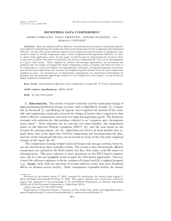
 Andrea Farruggia