


Abstract
Many processes during the evolution of protoplanetary disks and during planet formation are highly sensitive to the sizes of dust particles that are present in the disk: the efficiency of dust accretion in the disk and volatile transport on dust particles, gravoturbulent instabilities leading to the formation of planetesimals, or the accretion of pebbles onto large planetary embryos to form giant planets are typical examples of processes that depend on the sizes of the dust particles involved. Furthermore, radiative properties like absorption or scattering opacities depend on the particle sizes. To interpret observations of dust in protoplanetary disks, a proper estimate of the dust particle sizes is needed. We present DustPy: a Python package to simulate dust evolution in protoplanetary disks. DustPy solves gas and dust transport including viscous advection and diffusion as well as collisional growth of dust particles. DustPy is written with a modular concept, such that every aspect of the model can be easily modified or extended to allow for a multitude of research opportunities.
Export citation and abstract BibTeX RIS

Original content from this work may be used under the terms of the Creative Commons Attribution 4.0 licence. Any further distribution of this work must maintain attribution to the author(s) and the title of the work, journal citation and DOI.
1. Introduction
Dust plays an important role in many processes of planet formation. Interstellar micrometer-sized dust particles accumulate in protoplanetary disks due to angular momentum conservation and grow to millimeter-sized pebbles via collisional growth. However, various growth barriers prevent particles from growing directly into planetesimals, e.g., the charge barrier, the bouncing barrier, the drift barrier, or the fragmentation barrier. As soon as particles reach millimeter sizes gravoturbulent instabilities can play an important role. These instabilities have the ability to concentrate particles in pebble clouds, which can subsequently collapse under their own gravity into planetesimals if they are massive enough (see Youdin & Goodman 2005; Johansen et al. 2007). These planetesimals can collide to form larger bodies and eventually planetary embryos. Leftover dust pebbles in the disk accrete onto these embryos to assemble terrestrial planets or the cores of giant planets (see Ormel 2017).
The efficiency of said processes like planetesimal formation (Krapp et al. 2019; Paardekooper et al. 2020) or pebble accretion onto planetary embryos (Liu & Ormel 2018; Ormel & Liu 2018) is highly sensitive to the sizes of dust particles available in protoplanetary disks. To understand the formation of planets and to interpret the population and composition of observed exoplanets it is therefore crucial to know which particle sizes can exist at any specific time and location in the lifetime of protoplanetary disks. Furthermore, it is important to understand the size evolution of dust particles when interpreting observations of dust in protoplanetary disks (Sierra et al. 2021).
To simulate the collisional evolution of micrometer-sized dust particles up to planets it is unfeasible to simulate every dust particle individually. Several techniques have been developed in the past to overcome this. One is the Monte Carlo method wherein several dust particles are combined into a few representative particles, whose evolution can be simulated (see Ormel et al. 2007; Zsom & Dullemond 2008; Drażkowska et al. 2013). Another method is to simulate the evolution of a particle size distribution instead of individual particles (see Weidenschilling 1980; Nakagawa et al. 1981; Dullemond & Dominik 2005; Brauer et al. 2008; Birnstiel et al. 2010). The advantage of Monte Carlo methods is that it is relatively easy to include additional particle properties like electrical charge, porosity, or composition, while this is a rather complex task in the case of particle distributions (see Okuzumi et al. 2009; Stammler et al. 2017). Monte Carlo methods, however, are computationally expensive, while methods with particle distributions can cover longer time spans of disk evolution.
We developed the Python package DustPy, 3 which simulates the evolutions of a dust mass distribution in protoplanetary disks accounting for collisional growth and transport of dust particles, as well as the evolution of the gas disk. It can be used to simulate the evolution of the gas and dust within a protoplanetary disk over its entire life span.
The main object of DustPy is to calculate the evolution of the gas surface density Σg and Nm dust surface densities Σd,i of different particle masses in a protoplanetary disk with Nr radial grid cells, including viscous evolution of the gas, advection and diffusion of the dust, as well as collisional dust growth by solving the Smoluchowski equation. It is therefore one-dimensional in space. DustPy itself uses the Simframe framework for scientific simulations (Stammler & Birnstiel2022), which allows the user to easily customize every aspect of the model or to extend it with additional functionality. This publication, therefore, discusses the default functionality of DustPy, i.e., the model that is run without any customization. DustPy is written in Python to allow for easy access and great flexibility. Computationally expensive routines are written in Fortran. However, the main focus is on usability, not on optimizing the execution time.
This publication is structured as follows. Section 2 introduces the relevant equations for gas evolution. In Section 3 we discuss dust evolution, which consists of two major parts: dust transport in Section 3.1 and collisional dust growth in Section 3.2. In Section 4 we compare the coagulation algorithm of DustPy to test cases that have analytical solutions. In Section 5 we present example simulations that show the full potential of DustPy customizations. Finally, in Section 6 we summarize the features and caveats of DustPy.
2. Gas Evolution
DustPy assumes an axisymmetric disk. All quantities, therefore, only have one spatial coordinate, the radial distance r from the star. If applicable, DustPy assumes vertical hydrostatic equilibrium in the z direction, i.e., the height above the midplane of the disk. By default, DustPy viscously evolves the gas surface density via the viscous advection-diffusion equation

including external source terms Sext, which can be used to implement, for example, infall of matter onto the disk or losses due to photoevaporation. In the default model Sext is set to zero. The radial gas velocity is given by

with the Keplerian velocity  and the viscous accretion velocity given by Lynden-Bell & Pringle (1974) as

with the kinematic viscosity ν. G is the gravitational constant and M* the mass of the central star. In the default DustPy model the kinematic viscosity is given by  , with the α viscosity parameter introduced by Shakura & Sunyaev (1973), the sound speed cs, and the Keplerian frequency
  . η is the pressure gradient parameter, given by

with the pressure scale height  . The parameters A and B in Equation (2) are used to implement the dynamic back reaction of dust particles onto the gas. In the default model DustPy uses A = 1 and B = 0, i.e., no back reaction. This is accurate as long as the dust mass is small compared to the gas mass. With decreasing A and increasing B, gas accretion can be halted or even reversed. Gárate et al. (2020) implemented back reaction of dust particles onto the gas in a region with an increased dust-to-gas ratio caused by a "traffic jam" at the line into DustPy. For details on the implementation of A and B we refer to that publication.
2.1. Algorithm
Equation (1) can be discretized and written as a matrix equation implicitly in  , where the superscript n represents the time coordinate

The Jacobian  is a tri-diagonal matrix, since the radial grid cells only interact with themselves or with neighboring grid cells.
A sketch of the Jacobian  can be seen in Figure 1. Exceptions to the tri-diagonal shape of the Jacobian are the first and the last rows, which are used to set the boundary conditions. By default the inner boundary is set to a constant gradient, while the outer boundary is set to the gas floor value to prevent inflow of gas through the outer boundary. Since most of the elements of
  are zero, DustPy uses the scipy.sparse package (Virtanen et al. 2020) to store the Jacobian in a sparse matrix format.

Figure 1. Sketch of the gas Jacobian in an example with 15 radial grid cells. The Jacobian consists of the main diagonal and one upper and one lower off-diagonal, because the gas can only interact with itself or with neighboring grid cells. Exceptions are the first and the last rows, which are used to set the boundary conditions.
Download figure:
Standard image High-resolution imageEquation (5) can be solved for  via
via

by inverting the matrix  . To achieve this, the matrix is factorized with scipy.sparse.linalg.splu, before solving the system of equations with scipy.sparse.linalg.SuperLU.solve.
3. Dust Evolution
Dust evolution in DustPy consists of two parts: dust transport and dust growth. Dust transport is calculated by solving the advection-diffusion equation, similar to gas evolution. Dust growth is calculated by solving the Smoluchowski equation. The dust quantities consist of Nm different dust species of different masses at every radial position.
3.1. Dust Transport
To account for dust transport DustPy solves the advection-diffusion equation (Clarke & Pringle 1988) for every dust species i:

The radial dust velocity vd,i is given by

with the maximum drift velocity given by

where A and B are the back reaction coefficients introduced in Equation (2). The Stokes number, Sti , is a measure of the aerodynamic size of a dust particle. DustPy considers by default two aerodynamic drag regimes: the Epstein and the Stokes I regimes:

with the dust particle radius ai , the dust bulk density ρs,i , and the mean free path of the gas λmfp. The Stokes I regime is typically only important for large particles in the inner parts of protoplanetary disks. The dust diffusivity in Equation (7) is taken from Youdin & Lithwick (2007) and is given by

The parameter δr describes the strength of radial diffusion of the dust particles and is similar to the turbulent α parameter.
3.2. Dust Growth
Modeling collisional dust growth in protoplanetary disks is challenging. To form an Earth-like planet out of micrometer-sized dust particles one would need to simulate the evolution of about 1040 individual dust particles, which is not feasible. To overcome this problem a number of strategies have been developed in the past. One is the so-called Monte Carlo method, in which many physical particles are combined into a few representative particles whose evolution can be calculated (see Ormel et al. 2007; Zsom & Dullemond 2008; Drażkowska et al. 2013).
DustPy, on the other hand, calculates dust growth by solving the Smoluchowski equation:

Instead of tracking individual particles, DustPy calculates the collisional evolution of a distribution  of particles with masses m. The first double integral on the right-hand side sums over all possible collisions of particles with masses
  and
and  and collision rate
  . The matrix
  holds information about the collision outcomes of each collision and describes the amount that gets added into
  from a single collision of particles with masses
  and
and  . A perfectly sticking collision would be described with
  .
.
The upper boundary of the inner integral is  instead of ∞ , because collisions of particles with masses
  and
and  are identical to collisions of particles with masses
  and
and  and should not be counted twice. The negative term on the right-hand side accounts for the particles that get removed from the distribution, because they have collided with other particles.
DustPy discretizes  on a mass grid with Nm
mass bins by integrating
on a mass grid with Nm
mass bins by integrating  over the mass bin width:

With this the discretized Smoluchwoski equation can be written as

Please note the Kronecker δ in the second term on the right-hand side. For equal particle collisions  two particles from the same mass bin have to be removed from the distribution.
This section discusses the various challenges in implementing Equation (14) into the numerical algorithm of DustPy. This is rather technical. Readers that want to skip the derivation can continue reading at Section 3.2.3. In a typical DustPy simulation the user does not need to modify the collisional subroutines, unless the goal is to implement a custom collision model.
3.2.1. Coagulation
The case of pure coagulation, i.e., perfect sticking of two particles forming a new larger body, has a number of computational challenges. First, the mass grid of DustPy is logarithmically spaced to cover a large dynamic range from submicrometer-sized particles to large boulders. This has the disadvantage that the resulting mass of two colliding particles mcoll = mi + mj will in general not fall exactly onto the mass grid itself, but in between two mass bins. We follow the approach of Brauer et al. (2008) to linearly distribute the newly formed particle between the two adjacent mass bins. Assuming the mass of the particle resulting from a sticking collision of particle mi and mj falls in between the two mass bins mm ≤ mcoll < mn , we split the coagulation rate linearly between both mass bins:

where  is given by

If mcoll = mm
⇒ = 1 and the entire particle will be distributed into mass bin mm
. Since by definition mn
> mcoll, mass will always be distributed into a mass bin that is larger than the combined mass of the colliding particles, leading to artificial growth. The mass grid, therefore, needs to be fine enough to limit this numerical inaccuracy. This limitation is discussed in Section 4.1 in more detail.
Another challenge is purely computational and is caused by the limited precision of computers. For double-precision numbers, for example, we face the problem that mi + mj = mi , if mi is more than 15 orders of magnitudes more massive than mj . This would prevent large particles from growing by sweeping up many small particles. This problem can be solved by rearranging the sums in the discrete Smoluchowski equation. We, again, follow the approach of Brauer et al. (2008). Figure 2 shows a sketch of three types of particle collision that are dealt with separately in this section.
Starting from Equation (14) we can separate the diagonals from the first term on the right-hand side, i.e., the equal-mass particle collisions, and combine it with the Kronecker δ of the negative term:

The superscript "s" denotes that these are the source terms and collisions rates for purely sticking collisions. The sum over i does not need to go all the way to Nm but only up to k, because sticking collisions involving particles larger than mk can never positively contribute to nk . We now look more closely at the second and third terms on the right-hand side and separate the case k = i from the second term, i.e., those collisions that can be affected by machine-precision errors, when a large particle with mass mk is sweeping up a small particle mj such that the resulting mass is in between mk and mk+1:

The second term on the right-hand side with Kkjk represents these special collisions for which particles with masses mk and mj collide, but still have a positive contribution to nk (type 1 in Figure 2). The term only describes particle collisions for which mk + mj ≤ mk+1, otherwise the resulting mass of the collision would be too large to positively contribute to nk . We therefore introduce a number, c, which is defined as the smallest integer for which the condition mk + mk+1−c ≤ mk+1 is fulfilled. In general, c would depend on k. But since the mass grid of DustPy is regular logarithmic, c will be a constant as long as the mass grid does not change. We can now replace the upper boundary of the sum in the second term with k + 1 − c and combine it with the respective negative part of the sum in the third term:

Please note that c ≥ 2, since the equal-size collisions  are already included in the first term in Equation (17). In any case, mass grids with Kkkk
≠ 0 that lead to mk
≤ mk
+ mk
< mk+1 would have fewer than
are already included in the first term in Equation (17). In any case, mass grids with Kkkk
≠ 0 that lead to mk
≤ mk
+ mk
< mk+1 would have fewer than  mass bins per decade. Simulations should have at least seven mass bins per decade for simple collision models (Ohtsuki et al. 1990), and even more for complex collision models (Drażkowska et al. 2014). Further, note that the collision rates are symmetric, i.e.,
  . Collisions of particle mj
with mk
occur at the same rate as collisions of particle mk
with mj
. Since Kkjk
in the first term means that mk
≤ mk
+ mj
< mk+1 we can set mm
= mk
and use Equation (15) to get
. Collisions of particle mj
with mk
occur at the same rate as collisions of particle mk
with mj
. Since Kkjk
in the first term means that mk
≤ mk
+ mj
< mk+1 we can set mm
= mk
and use Equation (15) to get

In collisions prone to machine-precision errors, a computer would falsely calculate mk + mj = mk . Already manipulating Kkjk − 1 in advance in these collisions eliminates these errors. Using this for the first term and combining it with the second term, we get

with

Up to this point the coagulation equation reads

Now we look at the second term on the right-hand side for the case i = k − 1:

These are the other types of collision that can be affected by machine-precision errors. In this case particles with masses mk−1 and mj collide and have a positive contribution to nk . We can distinguish two cases here. In the first case the resulting mass of the colliding particles falls in between mk−1 ≤ mk−1 + mj < mk (type 2a in Figure 2). This means mk = mn in Equation (15) and therefore

These collisions are identical to type 1 but look at the mass that is distributed into the larger mass bin. In the second case the resulting mass falls in between mk ≤ mk−1 + mj < mk+1 (type 2b in Figure 2). Here we have mk = mm in Equation (15) and therefore

Cases with mk−1 + mj
> ≥ mk+1 do not contribute positively toward nk
. The Heaviside step function takes care of these cases. In both cases either 1 − or itself can be affected by machine-precision errors. It is therefore advisable to manipulate directly these cases in advance, as shown above. We can now split the sum into both cases using the constant c that has been introduced earlier:

The matrix E is given by

The full coagulation equation now reads

It is useful to bring the equation into a double sum form:

where the Kronecker δ and the Heaviside step function Θ are used to pick the correct values and ranges for i and j. In that way the coagulation equation can be written with one single double sum. Note that the inner sum has to go up until Nm
, because the matrices Dji
and Ejk
are not symmetric. Since i and j are integer numbers, the terms of  and
and  in the Heaviside step functions are used to avoid a potentially undefined behavior for
  .
.

Figure 2. Sketch of the mass grid with three special types of collisions highlighted. Type 1: particle of mass mj collides with particle of mass mk with the resulting mass being between mk and mk+1. Type 2a: particle of mass mj collides with particle of mass mk−1 with the resulting mass being between mk−1 and mk . Type 2b: particle of mass mj collides with particle of mass mk−1 with the resulting mass being between mk and mk+1.
Download figure:
Standard image High-resolution imageFrom a computational perspective it is beneficial to bring the equation into a symmetrical form to save half of the iterations. DustPy, therefore, solves the following equation:

with

and

Please note that diagonal entries  must not be counted twice. All diagonals need therefore a factor of
  . Only the first two terms of Equation (30) contain diagonals. The first term contains only diagonal entries, while the second term contains both diagonal and off-diagonal entries. However, since c ≥ 2, this means for the diagonals of the second term Dkk
= −1. This is one particle that gets removed from the distribution in collisions with two equal-size particles. The other particle is removed by δik
in the first term of Equation (30). We can therefore omit the δik
in the first term and the factor of
. Only the first two terms of Equation (30) contain diagonals. The first term contains only diagonal entries, while the second term contains both diagonal and off-diagonal entries. However, since c ≥ 2, this means for the diagonals of the second term Dkk
= −1. This is one particle that gets removed from the distribution in collisions with two equal-size particles. The other particle is removed by δik
in the first term of Equation (30). We can therefore omit the δik
in the first term and the factor of  for the second term in Equation (33).
For any given collision of particles with masses mi and mj , Cijk will either have zero, three, or four nonzero elements. Cijk will always have two positive entries for k = m and k = n (the two mass bins in between which the resulting collisional mass falls) and negative entries for k = i and k = j (the colliding particles), leading to four nonzero entries. In special cases, when i = j, k = i, or k = j, this number can be reduced to three. If mi + mj is larger than the largest mass of the mass grid Cijk will be set to zero to prevent mass loss through the upper boundary of the mass grid.
A peculiar property of Cijk for any particle collision is

Since the coagulation equation described above works on number densities, the sum of Cijk over k for any combination of i and j has to be −1 as long as the mass of the colliding particles is within the mass grid. Two particles collide, stick, and form a single larger particle. Therefore, for every sticking collision the total number of particles is reduced by one.
Cijk
only needs to be calculated once in the beginning of the simulation as long as the mass grid does not change. Because there are a maximum of four nonzero elements for any combination of i and j, the coagulation problem is of the order  .
.
Equation (31) can be written in matrix form:

with the sticking Jacobian Js being defined as

A sketch of the structure of the Jacobian with the contributions of the four terms in the definition of  in Equation (33) is shown in Figure 3 for a mass resolution of seven mass bins per decade. The last column is always empty, since collisions with particles of mass
  will always result in a particle exceeding the mass grid. In this setup the element J21 is empty, because it represents collisions involving at least one particle of mass m1 that have a positive contribution to n2. However, the mass grid is fine enough, such that m1 + m1 > m3, which means that n2 cannot be filled from these types of collisions. The first term represents equal particle collisions, the second term contains the
  matrix with the negative contributions to the distribution, the fourth term contains the contribution of the
  matrix, and the third term contains the remaining collisions.

Figure 3. Sketch of the sticking Jacobian with the contributions of the four terms in Equation (33).
Download figure:
Standard image High-resolution image3.2.2. Fragmentation
If the relative velocity of the colliding particles exceeds the fragmentation velocity, particles fragment rather than stick and grow. DustPy distinguishes by default two types of fragmentation events: full fragmentation and erosion.
Full fragmentation means that both colliding particles fully fragment, leaving behind a fragment distribution that follows a power law:

The exponent γ has to be determined experimentally. DustPy uses by default  , taken from Dohnanyi (1969). Erosion, on the other hand, happens when both colliding particles differ significantly in mass. The smaller projectile particle then fully fragments while chipping off some mass from the larger target particle. The outcome of a erosive collision is a fragment distribution and a slightly less massive remnant target particle. In DustPy the transition between full fragmentation and erosion is by default at a particle mass ratio of 10.
To calculate the contribution of fragmenting collisions, DustPy uses the  algorithm developed by Rafikov et al. (2020). We slightly modified the algorithm to make it strictly mass conserving and to account for the DustPy code units, where the dust quantities are integrated over the mass bin. For this purpose we define a normalized fragment distribution:

φij is the amount that gets added to nj from a fragment distribution with a total mass 1 and a largest fragment mass of mi . The Heaviside step function sets φij to zero if the index j is greater than the largest mass bin of the fragment distribution. The exponent is 1 + γ instead of γ, because the quantity is integrated over the mass bin. As another quantity we define the total mass of fragments that is created in a single particle collision event:

For fully fragmenting collisions the fragment mass is the total mass of the colliding particles. For erosive collisions the projectile particle chips off a fraction of χ of its own mass from the target particle. In DustPy χ = 1 by default. Without loss of generality, mj is always the mass of the smaller projectile particle. Another quantity that is needed is the largest mass, mk , of the fragment distribution. The index of the largest fragment is given by

In fully fragmenting collisions the fragment distribution goes all the way up to the largest particle. In erosive collisions, the largest particle of the fragment distribution has the mass of the projectile particle. With these quantities we can now sum up the contribution of all collisions to the total fragment distribution multiplied with their individual fragment mass and weighted by their collision rates and store them in a vector,  , at the position of the largest fragment:

where the superscript "f" denotes the collision rates for fragmenting collisions. The contribution from fragments of all collisions into nk is then given by

In both cases, full fragmentation and erosion, the smaller projectile particle will fully fragment and has to be removed from the particle distribution:

Similarly, the larger target particle has to be removed in fully fragmenting collisions. In erosive collisions, however, the target particle has to be removed from the distribution and then added, as a remnant particle, at another place in the distribution:

The matrix  is similar to Kijk
in Equation (15) from the previous section and decides between which two mass bins the remnant particle has to be distributed, but with the mass of the remnant particle instead of the total mass of both collision partners. If the remnant particle has a mass mi−1 ≤ mi
− χ
mj
< mi
, mass would be removed and then added into the target particle's mass bin ni
. If that is the case, a similar manipulation as for the coagulation can be performed to avoid machine-precision errors. Since the mass grid of DustPy is logarithmically spaced and the transition between full fragmentation and erosion is defined by the mass ratio of the colliding particles, we can define a constant p, such that full fragmentation happens if j ≥ i − p:
is similar to Kijk
in Equation (15) from the previous section and decides between which two mass bins the remnant particle has to be distributed, but with the mass of the remnant particle instead of the total mass of both collision partners. If the remnant particle has a mass mi−1 ≤ mi
− χ
mj
< mi
, mass would be removed and then added into the target particle's mass bin ni
. If that is the case, a similar manipulation as for the coagulation can be performed to avoid machine-precision errors. Since the mass grid of DustPy is logarithmically spaced and the transition between full fragmentation and erosion is defined by the mass ratio of the colliding particles, we can define a constant p, such that full fragmentation happens if j ≥ i − p:

The first term now holds both the positive and the negative contribution for the target particle from erosive collisions. We can distinguish two cases. In the first case the positive and negative contributions can be combined, since they both affect the same mass bin:
1. mi−1 ≤ mi − χ mj < mi :

2. mm ≤ mi − χ mj < mn < mi :

The full equation for fragmentation and erosion is therefore the sum of all three contributions:

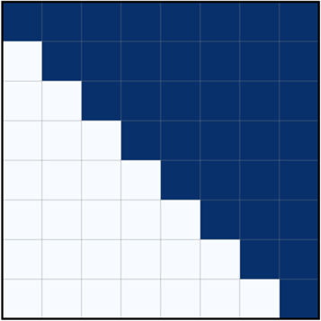
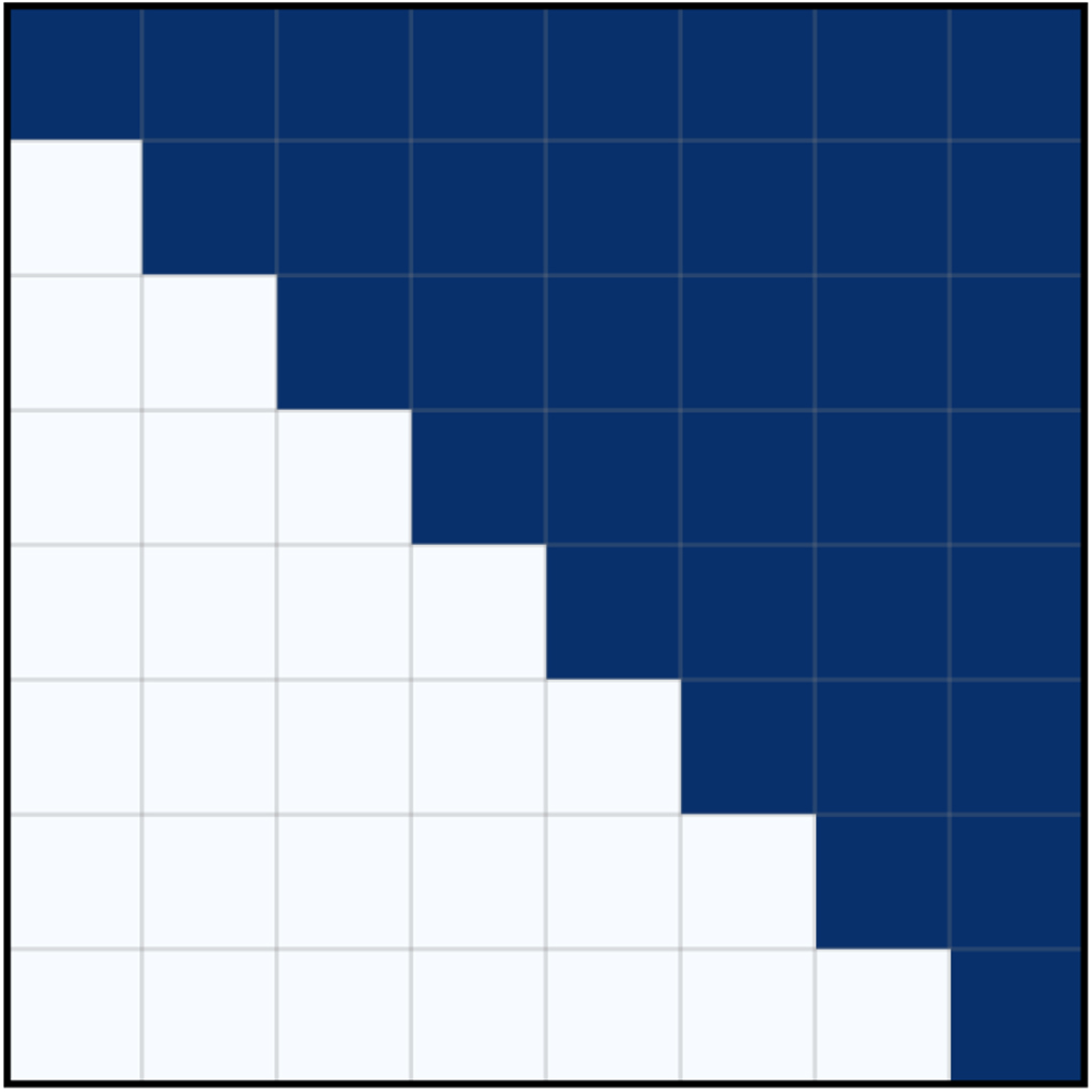
The source terms of fragmentation can also be written in matrix form. A sketch of the fragmentation Jacobian is shown in Figure 4 for a model where every collision leads to a fragmentation event. The fragmentation Jacobian is a simple upper triangular matrix.

Figure 4. Sketch of the fragmentation Jacobian.
Download figure:
Standard image High-resolution imageThis fragmentation and erosion prescription is of the order  . The full dust growth equation can then be simply combined to

with the dust Jacobian being the sum of the sticking and fragmentation Jacobians:

3.2.3. Collision Rates
The collision rates for sticking/fragmenting collisions are the product of the geometrical cross section, the relative velocities of the particles, and the sticking/fragmentation probabilities, respectively:

with  . However, please note that the DustPy quantities are vertically integrated, which has been ignored so far. Vertical integration of the Smoluchowski equation introduces a correction factor, which will be incorporated into the collision rates. This is discussed in Section 3.2.6 in more detail. Further note, that a population of N equal-sized particles has
  possible collisions amongst each other, which is
  in the limit of large N. Equal particle collisions, therefore, need a factor of
  , which is incorporated via the
  in the collision rates in Equation (51).
3.2.4. Relative Velocities
DustPy considers by default five different sources of relative velocities between dust particles: Brownian motion, radial and azimuthal drift, vertical settling, and turbulence.
Figure 5 shows all five contributions to the relative velocities in an example simulation of the default DustPy model at a distance 1 au from the star. Brownian motion is especially important as a driver of initial dust growth, when the particles are rather small.

Figure 5. Example of the different sources of relative velocities in the default model of DustPy at a distance of 1 au.
Download figure:
Standard image High-resolution imageBrownian motion. The relative velocities due to Brownian motion are given by

Since this formula is diverging for very small particle masses, the relative velocities are limited to the sound speed cs. However, one should note that for very small particles and high temperatures, the relative velocities due to Brownian motion can easily exceed typical values for the fragmentation velocity. In the simple collision model that is used by default in DustPy, there is no distinction on particle size when deciding between sticking and fragmentation. Even though these small particles would in reality still stick (or bounce) at these velocities (Chokshi et al. 1993; Blum & Wurm 2008), DustPy would treat those collisions as fragmentation events.
Azimuthal drift. Since dust particles of different sizes have different degrees of sub-Keplerian motion, this leads to a relative velocity in azimuthal direction, which is given by

Dust particles of the same Stokes number do not experience any relative velocity due to azimuthal drift, because they drift at the same speed.
Radial drift. Dust particles of different sizes have different radial drift speeds. This induces relative velocities between dust particles. They are given by

with the radial dust velocities from Equation (8).
Vertical settling. Dust particles of different sizes settle with different velocities toward the midplane. DustPy uses the descriptions of Dullemond & Dominik (2004) and Birnstiel et al. (2010) to account for this effect:

where hi is the dust scale height, given by Dubrulle et al. (1995) as

δz is the vertical settling parameter similar to the turbulent α parameter.
Turbulent motion. To calculate the relative velocities due to turbulent motion we follow the prescription of Ormel & Cuzzi (2007). Instead of the turbulent α parameter we use the δt parameter, which works in an identical way but allows us to disentangle both effects.
The total relative velocity is then the quadratic sum of all contributions:

3.2.5. Coagulation/Fragmentation Probabilities
If the relative collision velocity exceeds the fragmentation velocity, particles start to fragment instead of growing to larger bodies. In the default DustPy model the fragmentation velocity is set to vfrag = 1 ms−1.
Different particles, however, do not collide with a single relative velocity as described in Section 3.2.4. Instead, the relative velocities follow the Maxwell–Boltzmann distribution:

with the rms velocity vrms, which DustPy assumes to be the single velocity derived in Section 3.2.4.
The collision rate for fragmenting collisions described in Section 3.2.3 would therefore be an integral over all possible relative velocities in the Maxwell–Boltzmann distribution, which are above the fragmentation velocity:

This integral has an analytical solution, and therefore the fragmentation probability in Equation (51) can be written as

with the mean velocity of the Maxwell–Boltzmann distribution  . In that way, it is sufficient to only calculate one relative velocity per particle collision while accounting for the velocity distribution in the fragmentation probability.
The sticking probability is then given by

Bouncing, i.e., neither sticking nor fragmentation, is not included in the default model of DustPy, but can be easily implemented if  . Figure 6 shows the Maxwell–Boltzmann distribution in the case of an rms velocity equal to the fragmentation velocity and the sticking/fragmentation probabilities for different relative velocities.

Figure 6. Left: Maxwell–Boltzmann velocity distribution for a rms velocity of 1 m s−1. Assuming a fragmentation velocity of 1 m s−1, some of the particles may fragment while some others can still grow. Right: sticking and fragmentation probabilities depending on the rms velocity assuming a Maxwell–Boltzmann velocity distribution and a fragmentation velocity of 1 m s−1.
Download figure:
Standard image High-resolution imageThe same approach of a velocity distribution was used by Windmark et al. (2012), while Birnstiel et al. (2010) originally used a simple formula for the transition between sticking and fragmentation at the fragmentation velocity.
3.2.6. Vertical Integration
So far we have ignored the vertical dimension of the disk. The Smoluchowski equation discussed in previous chapters works on volume densities. DustPy, on the other hand, only has one spatial dimension, the distance from the star r. Here we describe the method of Birnstiel et al. (2010) in vertically integrating the Smoluchowski equation. We assume that the vertical dust distribution can be described with a Gaussian:

with the dust scale height hk given by Equation (56). Integration over z leads to

Every single term in the collisional dust source terms introduced in Sections 3.2.1 and 3.2.2 contain the product of two densities with the collision rates Rij ni nj . Integrating this term over z and assuming to zeroth order that the collision rates do not depend on z leads to

Vertically integrating the Smoluchowski equation can therefore be achieved by simply replacing the midplane volume densities ni
with the vertically integrated number densities Ni
and by multiplying the collision rates with a correction factor. The quantity  is stored as kernel in DustPy.
DustPy does not store the vertically integrated number densities but uses dust surface densities, which are simply given by

Note that by using surface densities instead of number densities, this introduces further mass factors in quantities like Cijk
,  , or Hijk
introduced above. This is straightforward to do, but increases the complexity of the equations presented here. We therefore refer the interested reader to the software for details on the implementation.
, or Hijk
introduced above. This is straightforward to do, but increases the complexity of the equations presented here. We therefore refer the interested reader to the software for details on the implementation.
Further note, that only the dust densities have been vertically integrated. Other quantities, like the relative velocities needed for  , are still calculated in the midplane. This is a valid simplification, since most of the mass will settle anyway rather quickly toward the midplane.
3.3. Algorithm
Similar to the gas evolution algorithm, dust evolution can be written as a matrix equation. To achieve this, the two-dimensional (distance and mass) dust surface densities are flattened into a one-dimensional vector:

With this definition the dust evolution equation can be written in an implicit form:

The Jacobian in the case of dust evolution consists of two parts, hydrodynamic transport and dust growth. This equation can be solved for the new dust surface densities via

by inverting the matrix  .
.
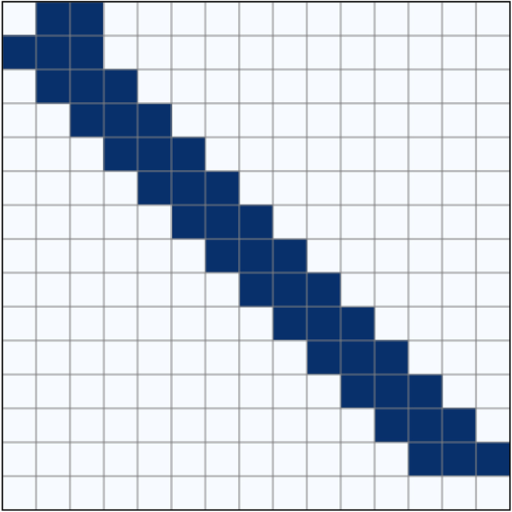
Figure 7 shows a sketch of the dust Jacobian in the case of six radial grid cells and eight mass bins. The Jacobian has a size of Nr Nm × Nr Nm . The large coarse boxes represent the radial grid cells, while the fine grids within the larger boxes represent the mass grid. As was the case for gas evolution, grid cells only interact with themselves or with neighboring radial grid cells for dust transport. These are the main diagonal and the off-diagonals that are Nm rows above and below the main diagonal.

Figure 7. Sketch of the dust Jacobian in an example with six radial grid cells and eight mass bins with only sticking and no fragmentation. The Jacobian has a size Nr Nm × Nr Nm . The 6 × 6 larger squares represent the radial grid, while the smaller 8 × 8 subgrids within each larger square represent the mass grid. Since for dust growth dust particles only collide with dust particles within the same radial grid cell, the Jacobian is only densely filled along the large diagonal squares. For dust transport particles only interact with dust particles of the same mass in the same and adjacent radial grid cells. This is represented in the Jacobian by the main diagonal and the two off-diagonals. The first Nm and last Nm rows are exceptions, since they are used to set the boundary conditions.
Download figure:
Standard image High-resolution imageIn the case of dust growth, mass bins can only interact with mass bins in the same radial grid cell. These are the filled boxes along the main diagonal in the Jacobian. The boxes are not completely filled, because in the case of sticking—that is shown here—not all collisions are possible. The Jacobian is set to zero for collisions that would result in particles that are larger than the mass grid. Furthermore, the lower-left triangle within a box is empty, because these terms have been added to the respective entries in the upper triangle to save loop iterations in the software.
The first Nm and last Nm rows of the Jacobian are used to set the boundary conditions without calculating coagulation here. In the default DustPy model the inner boundary is set to a constant gradient, while the outer boundary is set to a floor value. Diffusion is turned off at the boundaries by setting the diffusivity to zero.
Since most of the entries of the Jacobian are zero—in a typical simulation only about 1% of the Jacobian is filled—the Jacobian is stored in a sparse matrix format using scipy.sparse. To invert the matrix and solve the system of equations, in the default DustPy model the matrix is factorized with scipy.sparse.linalg.splu, before the equation is solved with scipy.sparse.linalg.SuperLU.solve. Factorizing the matrix before inversion reduced the runtime of the code in most cases.
Since, the inversion of a large matrix is computationally heavy, DustPy also has two additional options to integrate the dust quantities for large simulation sizes. The first option is to use the generalized minimal residual method, which is an iterative solver, for which DustPy uses scipy.sparse.linalg.gmres. The second option is to integrate the dust quantities explicitly using a fifth-order adaptive Cash–Karp integration scheme, which does not require the inversion of a matrix.
The timestep Δt is calculated such that neither the gas nor the dust densities could become negative in a first-order Euler scheme, while only considering the negative source terms  :
:

4. Test Cases
There are a few test cases with analytical solutions that can be used to benchmark DustPy against. In this section we compare the dust growth algorithm against two collision kernels with analytical solutions, and we compare the gas evolution algorithm against the self-similar solutions for viscous accretion.
4.1. Dust Coagulation
Starting from the Smoluchowski Equation (12):

and assuming perfect sticking, i.e.,  , leads to

This equation has analytical solutions for three special cases: the constant kernel  , the linear kernel
  , and the product kernel
  . The discretized form of this equation for pure sticking was derived in Section 3.2.1.
We will discuss the constant and the linear kernel in this section. The product kernel represents runaway growth that would quickly accumulate the entire mass of the system into a single particle, which cannot be properly addressed within DustPy as it uses particle distributions instead of physical particles. Solutions to the constant and the linear kernel are discussed in Silk & Takahashi (1979) and Wetherill (1990).
4.1.1. The Constant Kernel
The solution of Equation (71) with the constant kernel is given by

where m0 is the smallest possible mass and N0 the initial total number density of particles:

Note that the DustPy code units are the number densities integrated over the mass bin. We therefore initialize the simulation by setting the first mass bin to N0 and all other mass bins to zero.
The result is shown in Figure 8 (left panel) for a simulation with the default mass resolution of DustPy with dotted lines and for a simulation with a four times higher mass resolution with solid lines for α = 1. The analytical solutions given by Equation (72) are plotted with black solid lines. There is a slight deviation visible at the upper mass tail of the distribution in the default resolution run. An explanation for this is given at the end of the next section.

Figure 8. Comparison of the analytical solutions (black solid lines) of the constant kernel (left) and the linear kernel (right) to DustPy simulations with the default mass resolution (dotted colored lines) and with a four times higher mass resolution (solid colored lines).
Download figure:
Standard image High-resolution image4.1.2. The Linear Kernel
The solution of the linear kernel is given by

with N0 being the initial total number density as for the constant kernel and

Initially, only the first mass bin was filled with N0 while all other mass bins were set to zero.
The result is shown in Figure 8 (right panel) for a simulation with the default mass resolution of DustPy with dotted lines and for a simulation with a four times higher mass resolution with solid lines for α = 1. The analytical solutions given by Equation (74) are plotted with black solid lines. As for the constant kernel there is a deviation at the upper mass end of the distribution that is worse the lower the mass resolution is.
The reason for this is the algorithm described in Section 3.2.1. Since the mass grid is logarithmically spaced, the combined mass of both colliding particles in a sticking collision will not directly fall onto the mass grid itself, but has to be distributed between the adjacent mass bins as described in Equation (15). This leads to artificial growth, because material will be added to a bin that is more massive than the combined mass of the collision partners. This causes the simulations to be more massive at the higher mass end and—due to mass conservation—less massive at the lower mass end compared to the analytic solutions. The situation is worse for the linear kernel, because the kernel is proportional to the colliding mass itself. An overestimation of mass will overestimate the kernel itself.
But since the computational time is highly sensitive to the number of mass bins, one has to find a compromise between accuracy and execution time. For the simple collision model in the default DustPy simulation, the default mass resolution should be sufficient, since growth will be eventually halted by the fragmentation or by the drift barrier. Only the growth timescale might be slightly underestimated. For more complex collision models, including, for example, mass transfer, a higher mass resolution might be crucial. For more details on this we refer to Drażkowska et al. (2014), which performed mass resolution tests for more complex collision models. In any case, we advise to always run selected simulations with a higher mass resolution to verify that the default mass resolution was sufficient.
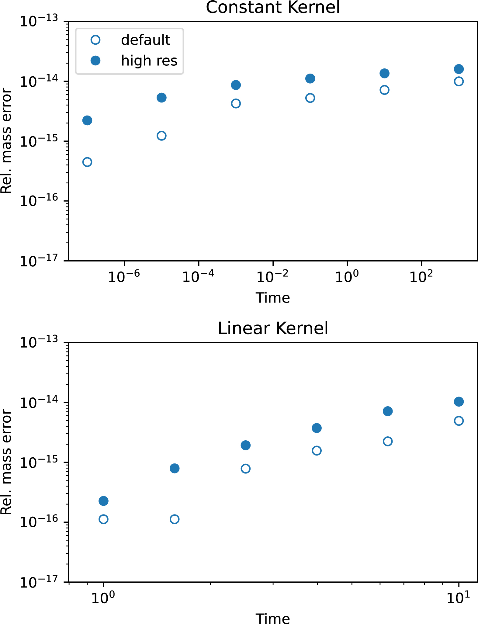
Figure 9 shows the relative errors in mass for the two benchmark models of the constant and linear kernels with the default and the high-resolution runs. In all cases the errors are very close to machine-precision levels for double-precision floating point numbers. The coagulation algorithm of DustPy is therefore mass conserving.

Figure 9. Relative error in mass in the benchmarks for the constant (top) and linear (bottom) kernels in the default (open circles) and the high-resolution (filled circles) runs.
Download figure:
Standard image High-resolution image4.2. Gas Transport
Viscous gas accretion as given by Equations (1) and (3) has an analytical solution, as discussed by Lynden-Bell & Pringle (1974) and Hartmann et al. (1998) and is given by

with the dimensionless time  , with a dimensionless scaling of the radial grid
  , and with the viscosity at the scaling location
  . γ is the exponent of the viscosity assuming it is a power law:

In the default DustPy simulation with s = 0 and  it follows that γ = 1. The scaling factor of time is given by

and the mass normalization factor

with M0 being the initial mass of the disk. We compare in Figure 10 a simulation with the default DustPy parameters against the analytical solution given by Equation (76). As can be seen, the result of DustPy is in good agreement with the analytical solution. Only in the last snapshot there is a small deviation close to the outer edge of the grid. The reason for this is that the outer gas boundary is set to the gas floor value, which is a very small number. This causes a minor underestimation of the surface density when the disk expands and reaches the outer boundary.

Figure 10. Comparison of the gas evolution of DustPy against the analytical solution of Equation (76).
Download figure:
Standard image High-resolution imageA word of caution on other slopes of the surface density: with the above default parameters of DustPy the surface density slope in the inner disk will be −1. If one wants to achieve slopes other than −1, it is not enough to simply change the initial surface density profile. Over time the surface density will approach −γ as given by Equation (77), since the viscosity profile determines the gas profile in the long run. One has to change the slopes of the viscosity or the temperature profile accordingly.
Similarly, the inner boundary has to be changed from a constant gradient to constant power law, for any other surface density profile than −1. For more details we refer to the documentation. 4
5. Examples
In this section we discuss selected examples of simulations performed with DustPy. The left panel of Figure 11 shows the default model of DustPy that is run when no parameter or function has been modified. The plotted snapshot is after 1 Myr. The quantity σd that is plotted is defined by

such that it is independent of the mass grid, since the code units of DustPy are integrated over the mass bin and therefore depend on the mass grid.

Figure 11. Example simulations of dust evolution with DustPy after a simulation time of 1 Myr. Left: the default model. Center: the default model with three ice lines changing the fragmentation velocity. Right: the default model including Jupiter and Saturn opening gaps.
Download figure:
Standard image High-resolution image
Table 1 lists the key parameters of the default model. But since DustPy is under continuous development, these parameters might be subject to change in the future. We would therefore like to refer to the documentation, 5

with the stellar radius and temperature R* and T*.
Table 1. Key Parameters of the Default DustPy Model
| Parameter | Description | Value | Equations |
|---|---|---|---|
| Rin | Inner grid boundary | 1 au | |
| Rout | Outer grid boundary | 1000 au | |
| Nr | Number of radial grid cells | 100 | |
| mmin | Minimum particle mass | 10−12 g | |
| mmax | Maximum particle mass | 105 g | |
| Nmbpd | Number of mass bins per decade | 7 | |
| M* | Stellar mass | 1 M⊙ | |
| R* | Stellar radius | 2 R⊙ | (81) |
| T* | Stellar effective surface temperature | 5772 K | (81) |
| Mdisk | Initial disk mass | 0.05 M⊙ | |
| p | Power law of surface density | −1 | |
| Rc | Initial critical cutoff radius | 30 au | |
| Initial dust-to-gas ratio | 10−2 | ||
| α | α-viscosity parameter | 10− 3 | (3) |
| δr | Radial mixing parameter | 10− 3 | (11) |
| δt | Turbulent mixing parameter | 10− 3 | |
| δz | Vertical mixing parameter | 10− 3 | (56) |

| Maximum initial particle size | 1 μm | |
| β | Initial particle size distribution 
| −3.5 | |
| γ | Fragment distribution | −11/6 | (37) |
| Mass ratio for erosion | 10 | ||
| ρs | Dust bulk mass density | 1.67 g cm−3 | |
| vfrag | Fragmentation velocity | 1 m s−1 | (60) |
| χ | Excavated erosive mass fraction | 1 | (39) |
Download table as: ASCIITypeset image
The blue line in Figure 11 is the fragmentation barrier. As particles grow their relative velocities increase, as shown in Figure 5. If their relative velocities exceed the fragmentation velocity, which is 1 m s−1 in the default model, the particles start to fragment instead of growing further. The fragmentation barrier is an estimate by Birnstiel et al. (2012) and is given by

where afrag is the maximum size a particle can reach at any location in the disk where particle growth is fragmentation limited.
The green line is the drift barrier. As seen in Equation (8), particles have increasing drift speeds with increasing Stokes numbers, i.e., with increasing size, until they reach the maximum drift speed at a Stokes number of unity. At some point the particles drift more rapidly toward the star, before they can grow to larger sizes. This is called the drift barrier and estimated by Birnstiel et al. (2012) as

where adrift is the maximum size particles can reach anywhere in the disk where growth is drift limited. The white lines in Figure 11 represent particle sizes with a Stokes number of unity, i.e., particles with the highest drift speeds and highest relative velocities. To achieve this simulation result only seven lines of Python code were needed including the import of modules and the initialization.
The center panel of Figure 11 shows the default model but with three ice lines at which the fragmentation velocity is changing. The model is similar to the model of Pinilla et al. (2017). The idea behind the model is that the fragmentation velocity of particles depends on their chemical composition, where icy particles could be more sticky than pure silicate particles (Schäfer et al. 2007; Wada et al. 2009). The adopted fragmentation velocity in this model is given by

Please note, however, that newer experiments suggest that the fragmentation velocity does not change that dramatically with composition (Musiolik & Wurm 2019). In regions with higher fragmentation velocity particles can grow to larger sizes, before they fragment. Since larger particles drift more rapidly, this depletes the outer disk rather quickly, enriching the inner disk inside the water ice line with material. To set up this model, only 14 lines of Python code were required, mainly to write a function for the fragmentation velocity. Please note further, that this example is only a showcase of the potential of DustPy and does not include evaporation and condensation of the molecules in question. It is relatively easy to include additional gas species in DustPy. The addition of new dust parameters like ice contents would require greater modifications to the dust distributions (see Okuzumi et al. 2009; Stammler et al. 2017).
The right panel of Figure 11 shows the default model but with Jupiter and Saturn inserted at their current locations. The planets open gaps in the gas disk and, since dust particles follow pressure gradients, the gap is also cleared of dust. It is difficult to achieve this gap opening in an one-dimensional simulation self-consistently. We therefore use the gap profiles provided by Kanagawa et al. (2017) obtained from two-dimensional hydrodynamical simulations. Since we also want to model gas accretion, we cannot simply set the gas surface density directly to these profiles. But since the product of the viscosity ν and the gas surface density Σ g is a constant in steady state, we can impose the inverse of the gap profile on the viscosity.
As seen in Figure 11, the planetary regions are cleared of gas. Since the Stokes number is inversely proportional to the gas surface density, the white line for particles of Stokes number unity is directly proportional to the gas surface density. The particles in the planetary regions have larger Stokes numbers due to the reduced gas surface density leading to higher relative velocities and therefore smaller particles sizes. To set up this simulation about 80 lines of Python code were necessary, where most of the code is needed to define the gap profiles of Kanagawa et al. (2017).
Further examples of research that have been done with DustPy include Stammler et al. (2019), which implemented planetesimal formation in dust rings at the outer edges of gaps to explain the observed optical depths in protoplanetary disks. In a similar model, Miller et al. (2021) showed that moving pressure bumps could explain the observations of wide exo-Kuiper belts. Gárate et al. (2020) implemented back reaction of dust particles onto the gas in DustPy to investigate the influence of dust enrichment at ice lines on the accretion rate. Pinilla et al. (2021) performed a parameter study on the α, δr , δt , and δz parameters to investigate their influence on the maximum particle sizes dust particles can reach. Drażkowska et al. (2021) used DustPy to benchmark a simple model for the prediction of the pebble accretion rate in protoplanetary disks.
6. Summary
We developed DustPy, a Python package to simulate dust evolution in protoplanetary disks. DustPy solves for viscous gas evolution, dust advection and diffusion, and dust growth by coagulation and fragmentation. Computationally expensive routines are written in Fortran and called from within the Python environment.
DustPy uses the Simframe framework for scientific simulations, which makes it easy to change every aspect of the code to allow for a multitude of research opportunities.
Dust growth is simulated by solving the Smoluchowski equation for a dust mass distribution. In contrast to Monte Carlo methods, which simulate the evolution of representative particles, the advantage of DustPy is its execution time. The default model of DustPy takes about 25 minutes to evolve a full protoplanetary disk for 100,000 yr. The Monte Carlo model of Drażkowska et al. (2013), for example, takes about 25 days to simulate an annulus within a protoplanetary disk for 30,000 yr with 100,000 representative particles. The advantage of Monte Carlo methods, however, is that it is straightforward to add additional parameters to them, such as porosity or ice fraction to the dust particles, while this requires greater modifications to the dust densities in Smoluchowski solvers (see Okuzumi et al. 2009; Stammler et al. 2017).
DustPy is a one-dimensional code that only has one spatial coordinate, the radial distance from the star, to simulate axisymmetric disks. Nonaxisymmetric features as reported by Drażkowska et al. (2021) can therefore not be modeled. The vertical extent of the disk—the height above the midplane—is assumed to be always in hydrostatic equilibrium. This assumption is good enough for most parts of the disk, but might be violated in parts, where the collisional timescale becomes significantly shorter than the mixing timescale (see Krijt & Ciesla 2016; Klarmann et al. 2018). Furthermore, sedimentation-driven coagulation by particles settling toward the midplane cannot be modeled (Zsom et al. 2011).
DustPy uses a logarithmic mass grid to cover large dynamic ranges from submicron interstellar medium grain sizes to meter-sized boulders. Particles resulting from hit-and-stick collisions will therefore not generally lie on the mass grid itself. Their mass will be added into the two adjacent mass bins. This will, however, artificially create particles that are too large. In the default model this will not be an issue since dust growth is halted by fragmentation and drift; only the growth timescale will be slightly underestimated. In more complex collision models, as in Windmark et al. (2012), where large particles can continue growing by sweeping up small particles, it is crucial to not overestimate the sizes of the largest particles. Other algorithms, like Lee (2000), Dullemond & Dominik (2005) or Lombart & Laibe (2021), may be better suited to conserve the shape of the particle distribution. The coagulation algorithm of DustPy, on the other hand, conserves the dust mass up to machine-precision. In any case, we advise users to always compare their results to high-resolution runs and check for convergence.
We thank the referee for their very helpful comments and suggestions as well as the rigorous cross-checking of the equations presented in this publication. The authors acknowledge funding from the European Research Council (ERC) under the European Union's Horizon 2020 research and innovation program under grant agreement No. 714769 and funding by the Deutsche Forschungsgemeinschaft (DFG, German Research Foundation) under grant Nos. 361140270, 325594231, and under Germany 's Excellence Strategy—EXC-2094-390783311.
Footnotes
- 3
DustPy repository: https://github.com/stammler/dustpy. Documentation: https://stammler.github.io/dustpy/. Installation of the latest version: pip install dustpyDustPy v1.0.1: https://doi.org/10.5281/zenodo.6874878.
- 4
Documentation: https://stammler.github.io/dustpy/.
- 5
Documentation: https://stammler.github.io/dustpy/. This will always list the most recent model parameters. The default temperature profile is that of a passively irradiated disk with an irradiation angle of 0.05.