
Abstract
Carbon budgets provide a useful tool for policymakers to help meet the global climate targets, as they specify total allowable carbon emissions consistent with limiting warming to a given temperature threshold. Non-CO2 forcings have a net warming effect in the Representative Concentration Pathways (RCP) scenarios, leading to reductions in remaining carbon budgets based on CO2 forcing alone. Carbon budgets consistent with limiting warming to below 2.0 °C, with and without accounting for the effects of non-CO2 forcings, were assessed in inconsistent ways by the Intergovernmental Panel on Climate Change (IPCC), making the effects of non-CO2 forcings hard to identify. Here we use a consistent approach to compare 1.5 °C and 2.0 °C carbon budgets with and without accounting for the effects of non-CO2 forcings, using CO2-only and RCP8.5 simulations. The median allowable carbon budgets for 1.5 °C and 2.0 °C warming are reduced by 257 PgC and 418 PgC, respectively, and the uncertainty ranges on the budgets are reduced by more than a factor of two when accounting for the net warming effects of non-CO2 forcings. While our overall results are consistent with IPCC, we use a more robust methodology, and explain the narrower uncertainty ranges of carbon budgets when non-CO2 forcings are included. We demonstrate that most of the reduction in carbon budgets is a result of the direct warming effect of the non-CO2 forcings, with a secondary contribution from the influence of the non-CO2 forcings on the carbon cycle. Such carbon budgets are expected to play an increasingly important role in climate change mitigation, thus understanding the influence of non-CO2 forcings on these budgets and their uncertainties is critical.

Original content from this work may be used under the terms of the Creative Commons Attribution 3.0 licence.
Any further distribution of this work must maintain attribution to the author(s) and the title of the work, journal citation and DOI.
1. Introduction
Limiting global mean warming to well below 2.0 °C in accordance with the Paris Agreement [1] requires a cap on the total amount of carbon dioxide emitted [2]. The Intergovernmental Panel on Climate Change [3,4] (IPCC) assessed such carbon budgets [3–7] based on CO2 alone, and accounting for all forcings. Those based on CO2 forcing alone were calculated from the Transient Climate system Response to cumulative carbon Emissions (TCRE), which was assessed from models and observations [3,8], while carbon budgets based on all forcings were calculated directly from RCP8.5 simulations. Here we compare 1.5 °C and 2.0 °C carbon budgets with and without accounting for the effects of non-CO2 forcings, evaluated using a consistent threshold-exceedance [7] approach from CO2-only and RCP8.5 simulations [9, 10]. We make use of simulations from eleven comprehensive Earth system models (ESMs) from the Fifth Coupled Climate Model Intercomparison Project [11] (CMIP5), driven by specified concentrations of CO2 and other greenhouse gases for the historical period and for the future period represented by the Representative Concentration Pathway 8.5 (RCP8.5) scenario [9, 10], which reaches a radiative forcing level of 8.5 W m−2 by year 2100, and includes forcing from both CO2 and non-CO2 agents (such as methane, nitrous oxide, halocarbons and aerosols; supplementary figure S1 available at stacks.iop.org/ERL/13/034039/mmedia), and prescribed land use change (Methods). Consistent with the IPCC approach [3, 7, 12], carbon dioxide emissions were diagnosed by summing increases in atmospheric, ocean and land carbon burdens and an estimate of land use change emissions [3, 9].
2. Methods
2.1. Cumulative emissions and carbon budgets
Cumulative carbon emissions (CE) were computed using the monthly mean output from the 1% per year CO2 increase (1PCTCO2), historical, and RCP8.5 prescribed CO2 simulations of the eleven CMIP5 Earth system models that had the data available, by addition of the net time-integrated atmosphere-land and atmosphere-ocean carbon fluxes, with the atmospheric burden and land use change emissions. Carbon budgets (CEB) are the cumulative carbon emissions consistent with limiting anthropogenic warming to below a specific temperature threshold (i.e. 1.5 °C or 2.0 °C, specified in text).
We make use of simulations from eleven comprehensive ESMs from the Fifth Coupled Climate Model Intercomparison Project [11] (CMIP5), including all models which had available output to compute cumulative carbon emissions from CO2-only and ALL-forcing simulations, as described below. The Earth system models used in this study include coupled carbon cycles. The ALL-forcing RCP8.5 simulations include specified land use changes [9]. These land use changes result in land use change emissions in the models [13], but these emissions cannot be diagnosed from the model output. Therefore, an estimate of the land use change emissions from the prescribed land-use change RCP8.5 scenario from the RCP database [9] was added to the total cumulative emissions, consistent to the approach used in the IPCC AR5 [12], in order to account for the carbon emissions from land use change that are simulated by the models forced with the RCP8.5 scenario, except for BCC-CSM 1.1 and BCC-CSM 1.1 m models, in which land use change is not prescribed, and therefore in which diagnosed emissions already correspond to total emissions.
In the 1PCTCO2 simulations [8], the atmospheric CO2 concentration increases at a rate of 1% per year for 140 years, starting from the pre-industrial value of approximately 285 ppm (specified to the exact value for each model, if such data was available). The ALL-forcing RCP8.5 simulation (ALL-forcing) includes prescribed concentrations of CO2, other greenhouse gases and aerosols (supplementary figure S1), and land use change [9], while the CO2-only simulations for CanESM2 are based on RCP8.5 CO2 forcing only.
The differences between the ALL-forcing simulation and the CO2-only simulation in the relationship between the temperature and the cumulative carbon emissions are shown in supplementary figure S2. We do not use the RCP 2.6 and RCP 4.5 simulations in our analysis, to avoid bias towards models that warm more strongly, because some of the RCP 2.6 simulations do not reach 1.5 °C global warming by 2100, and not all RCP 4.5 reach 2.0 °C. However, there are no significant differences between carbon budgets consistent with a given warming threshold computed from different RCP scenarios for low warming targets, since the ratio of CO2 to non-CO2 forcing does not vary very much across the different RCP scenarios in that case (supplementary figure S1).
2.2. Cumulative frequency distributions
Cumulative frequency distributions of carbon budgets (shown in figure 2) were calculated as in [14], according to equations 1.1 and 1.2 below. In equation 1.1 the carbon budgets (CEBl) simulated in individual ensemble members of all models considered are sorted in ascending order, and the cumulative frequency distribution is defined as:
where
and L is chosen such that CEBL < CEB < CEBL+1, I is the number of models considered, and Nl is the size of the ensemble from which the lth simulation is drawn. This approach uses all available ensemble members, but gives equal weight to each model [14]. If only one ensemble member is used from each model, it is identical to the approach used to generate a similar figure in the IPCC assessment ([3]: TFE.8, figure 1).
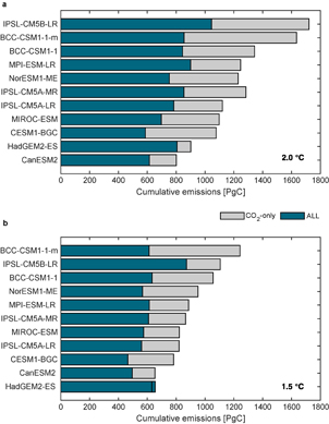
Figure 1. Cumulative carbon budgets in individual CMIP5 models. Cumulative carbon budgets consistent with limiting warming to 2.0 °C (panel a) and 1.5 °C (panel b) due to CO2-only forcing (grey bars), and ALL-forcing (blue bars) in RCP8.5 simulations of eleven CMIP5 models.
Download figure:
Standard image High-resolution image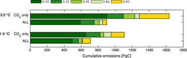
Figure 2. Cumulative frequency distribution of carbon budgets consistent with staying below 1.5 °C and 2.0 °C global mean warming relative to 1861–1880, based on eleven CMIP5 models and the RCP8.5 scenario. Top bars in each pair indicate carbon budgets based on CO2-only forcing from 1PCTCO2 simulations. Bottom bars in each pair indicate carbon budgets based on RCP8.5 simulations that include all forcings (‘ALL’). Cumulative frequency distributions were calculated from simulated CMIP5 carbon budgets as described in Methods. Note: the percentiles indicated in the legend refer to the right hand edge of each bar.
Download figure:
Standard image High-resolution imageThe probability density distributions (figure 3(b)) were calculated using Gaussian kernel density estimators, where the overall estimate of the PDF is based on the weighted sum of individual carbon budgets for each simulation (using the Silverman’s rule of thumb estimate of the standard deviation for each individual Gaussian). The individual Gaussians were scaled by the weights shown in equation 1.2. The probability density distributions for the IPCC carbon budgets reported in figure 3(a) are Gaussians fitted to the assessed 33%–66% ranges (figure 2; supplementary table S1).
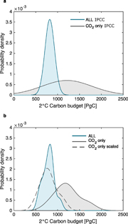
Figure 3. Comparison of 2.0 °C carbon budget probability density distributions. Blue curves indicate probability density distributions for carbon budgets based on simulations that include all forcings as in RCP8.5; grey curves are based on carbon budgets calculated for CO2 only (see Methods). The PDFs in panel (a) are based on IPCC AR5 values [3] (see Methods). Panel (b) shows PDFs based on the eleven CMIP5 models in this study, calculated using Gaussian kernel density estimators (see Methods).
Download figure:
Standard image High-resolution image2.3. Land use change in CanESM2
To diagnose land use change emissions in CanESM2, we derived the global integral of land-atmosphere carbon fluxes in an additional set of CanESM2 simulations, with prescribed changes in land use change only and atmospheric CO2 concentration held constant at the preindustrial level. This corresponds to the emissions caused by land use change alone, without conflating these with changes in land carbon due to changed atmospheric CO2. Since these simulations end in year 2006, for the subsequent years (until year 2040, before which both 1.5 °C and 2.0 °C targets are reached), we extended the land use change emissions using the RCP8.5 estimate of land use change emissions (supplementary figure S3(a)), and using the RCP8.5 land use change emissions estimate offset to agree with the mean of the model land use change emissions for the last decade before the historical period ends (supplementary figure S3(b)). The difference between these two estimates is only 5 PgC at the time of exceedance of 1.5 °C and 14 PgC at the time of exceedance of 2.0 °C. The land use change emissions diagnosed directly from the model output are lower than the RCP estimate of land use change emissions, but still within the uncertainty range of the observation-based land-use change emission estimates [15, 16]. The results presented in figure 4 and supplementary figure S4 depend on the representation of the terrestrial carbon cycle in the CanESM2 model, and are therefore model-dependent [13].
2.4. The effects of non-CO2 forcings on carbon budgets due to direct warming and due to land use change and carbon cycle
The reductions in CO2 only carbon budgets due to the effects of non-CO2 forcing occur due to a combination of the direct climate warming effects, and the combined effects of the land use change and the carbon cycle responses to additional warming. The combined carbon cycle feedback and land use change effect can be quantified by taking the difference between the cumulative carbon emissions in the ALL-forcing and CO2-only simulation in the year in which ALL-forcing simulation reaches the temperature target (supplementary figure S4, green arrow), since this directly represents the effect of non-CO2 forcings on the carbon emissions budget at the time of ALL-forcing threshold exceedance. The climate warming effect of the non-CO2 emissions on the budget can be quantified by noting that the warming caused by non-CO2 forcings is equal to the difference in temperature in the ALL-forcing and CO2-only simulation in the year in which the ALL-forcing simulation exceeds the threshold, or equivalently the warming simulated in the CO2-only simulation between the years in which the ALL-forcing simulations meets the threshold and the year in which the CO2-only simulation meets the threshold (as in [19]). The cumulative carbon emissions which would cause this much warming are hence the difference in cumulative emissions in the CO2-only simulation between the year in which ALL-forcing meets the threshold and the year in which CO2-only meets the threshold (supplementary figure S4, red arrow). The direct warming effect and the carbon cycle effect result together in the total difference in carbon budgets due to the non-CO2 forcings (supplementary figure S4, blue arrow).
3. Results
3.1. Distribution of carbon budgets
Carbon budgets consistent with a given warming threshold were assessed for each model by evaluating cumulative carbon dioxide emissions in the year prior to which the temperature threshold was first exceeded (figure 1, blue bars). Since carbon budgets calculated from CanESM2 simulations in which the atmospheric CO2 concentration increases at a rate of 1% per year (1PCTCO2) [8], give rise to statistically indistinguishable carbon budgets to those calculated based on CO2-only CanESM2 simulations with specified historical and future CO2 (supplementary figure S2; Supplementary figure S5; Methods), we calculated CO2-only carbon budgets for the eleven comprehensive Earth System Models in the same way from their respective 1% per year CO2 increase (1PCTCO2) simulations (figure 1, grey bars).
The results presented in figure 1 vary widely among different models, due to their different representations of carbon cycle processes. In particular, different representations of the terrestrial carbon cycle among the models [16] contribute to the differences among the carbon budgets calculated for the low warming climate targets. While most models exhibit CO2-only carbon budgets being greater than the ALL-forcing budgets (figure 1), due to net positive radiative forcing from non-CO2 forcings in the RCP8.5 scenario (supplementary figure S1), the ALL-forcing 1.5 °C carbon budget is actually greater than the CO2-only budget for the HadGEM2 model. Such behaviour likely arises from either a more negative aerosol radiative forcing and/or a greater sensitivity to that negative forcing.
Synthesizing results from all eleven models using an approach similar to that used by the IPCC [3, 7, 12] (Methods), carbon budgets consistent with limiting warming to 1.5 °C and 2.0 °C based on both CO2-only and ALL-forcing simulations, are shown in figure 2 as cumulative frequency distributions (Methods). Corresponding probability density functions (PDF) for 2.0 °C warming are shown in figure 3(b) (Methods; supplementary table S1). Comparing the 2.0 °C carbon budget PDF accounting for non-CO2 forcings calculated in this study (figure 3(b), blue PDF) with that reported by the IPCC [3] (figure 3(a), blue PDF), we note that the budgets in which non-CO2 forcings are accounted for are very similar, as expected, since we use a similar approach and set of CMIP5 simulations (Methods, supplementary table S1). Comparing budgets calculated in a consistent way with and without non-CO2 forcings, we find that accounting for the effects of non-CO2 forcings decreases the median carbon budget consistent with limiting warming to 1.5 °C by 257 PgC, and the median budget consistent with limiting warming to 2.0 °C by 418 PgC (figure 2, lower bars; supplementary table S1), similar to the 390 PgC decrease reported by the IPCC [3] (figure 3(a)).
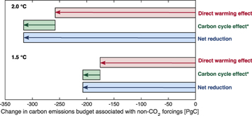
Figure 4. Separation of the effects of non-CO2 forcings on 1.5 °C and 2.0 °C carbon budgets in CanESM2. Red bars represent carbon budget reductions due to the direct warming effect, green bars represent reductions in carbon budget due to the net carbon cycle effect that includes carbon cycle feedbacks and land use change (Methods), and blue bars represent a net change in carbon budget (difference between red and green bars).
Download figure:
Standard image High-resolution image
3.2. Differences in ranges between CO2-only and ALL-forcing carbon budgets
While the difference in median budgets calculated here is similar to that reported by the IPCC, the carbon budget PDF consistent with limiting warming to 2.0 °C due to CO2-forcing alone, computed from the 1PCTCO2 simulations (figure 3(b), grey PDF) is much narrower than that reported by IPCC (figure 3(a), grey PDF): its 33%–66% range is 186 PgC, compared to 570 PgC. As explained in the IPCC assessment ([12], pg. 103), the IPCC-reported carbon budget range accounting for non-CO2 forcings is narrower than that of the IPCC-reported budget range for CO2-only in part because whereas the non-CO2 budget was estimated directly from the distribution of budgets in CMIP5 models, the CO2-only budget was inferred from an assessed range of TCRE. This TCRE range was itself based on CMIP5 models and observationally-constrained estimates, and with the range inflated to account for uncertainties not sampled over in CMIP5 models. However, our analysis shows that even when both sets of 2.0 °C carbon budgets are derived from CMIP5 simulations using a consistent approach, the 33%–66% spread based on ALL-forcing carbon budgets (figure 3(b), blue PDF) is narrower than that based on CO2-only simulations (figure 3(b), grey PDF) by a factor of two (see also supplementary table S1).
3.3. Understanding the narrower spread of ALL-forcing carbon budgets
To explore the factors contributing to this difference in the wide range of CO2-only carbon budgets, and much narrower range of carbon budgets from ALL-forcing simulations (figure 3), we explore the individual differences between CMIP5 models for CO2-only carbon budgets (from 1PCT CO2-simulations; figure 1 grey bars) and ALL-forcing carbon budgets (figure 1 blue bars), based on the RCP8.5 scenario. Why should there be less spread in the ALL-forcing budget compared to the CO2-only budget? If the temperature response to non-CO2 forcings simply scaled linearly with the temperature response to cumulative carbon emissions at the time of threshold exceedance in each model, then the ALL-forcing PDF would be a scaled version of the CO2-only PDF with its range scaled down by the ratio of the weighted mean budgets (dashed black line in figure 3(b)). Since the variances in this scaled PDF and the ALL-forcing PDF were not significantly different, this explanation is consistent with the narrower PDF seen for the ALL-forcing response. Thus, the narrower uncertainty ranges are explainable under the simplified assumption that the net warming response to non-CO2 forcings at the time of threshold exceedance is proportional to the net warming in response to CO2 in each model.
3.4. Separation of the effects of non-CO2 forcings on carbon budgets: due to direct warming, and due to carbon cycle effects
In the second part of this study we assess the mechanisms by which non-CO2 forcings influence cumulative carbon budgets. It is typically assumed that the effect of the non-CO2 forcings on cumulative carbon budgets is simply to increase the warming in a given year (direct warming effect), but these non-CO2 forcings are also expected to reduce the carbon uptake by terrestrial and marine carbon sinks through their additional net-warming effects, as shown in recent studies using an Earth system model of intermediate complexity [17–19]. Over land, warming increases both heterotrophic and autotrophic respiration from dead and live carbon components, respectively, but warming also generally adversely affects vegetation productivity in tropical regions [21], balanced in part by warming benefits to mid-high latitude vegetation where growth is currently limited by temperature. The net effect of all these processes is that warming leads to release of carbon from land. Over oceans, warming leads to a lower carbon uptake associated with reduced CO2 solubility in sea water [22]. In addition, warming leads to a stronger stratification of the upper layers of the ocean, which in turn, results in a lower ocean carbon uptake, due to reduced mixing between surface layer and deep waters, reducing the effective volume of the ocean that is exposed to high atmospheric CO2 [22]. We quantify these indirect effects of non-CO2 forcing on carbon budgets by comparing warming and diagnosed cumulative carbon emissions in prescribed-concentration RCP8.5 simulations of CanESM2 which include land use changes, with that in a similar set of simulations in which only CO2 varies and with no changes in land use (supplementary figure S2; Methods). Land use change emissions were calculated directly from CanESM2 simulations with specified land use change and prescribed preindustrial CO2 (see Methods), and were added to diagnosed fossil fuel emissions from the RCP8.5 simulations. Since the RCP8.5 simulations include both land use change and other non-CO2 forcings, effects of land use change on land carbon uptake could not be separated from effects of other non-CO2 forcings on land carbon uptake (Methods), therefore they are treated as a joint effect. Figure 4 separates the reduction in carbon budgets due to non-CO2 forcings (blue bars) into parts associated with climate warming (pink bars) and parts associated with carbon cycle changes (green bars).
The primary influence of the non-CO2 forcings is through climate warming (leading to reductions by 175 PgC and 258 PgC of the 1.5 °C and 2.0 °C carbon budgets due to the direct warming effect alone; supplementary figure S4), and their effect on carbon cycle feedbacks and carbon sinks is secondary. Reference [19] also reported reductions in carbon budgets due to non-CO2 forcings on carbon cycle feedbacks to be less than the reductions due to the climate warming of non-CO2 forcings, using an Earth system model of intermediate complexity [19]. Greater reductions in the CO2-only carbon budgets due to the climate warming effect are projected for higher temperature targets (figure 4), as the net warming effect of non-CO2 forcings increases with time in the RCP scenarios (due to declining aerosol forcing; supplementary figure S1). Since the representation of terrestrial carbon processes largely varies between different CMIP5 models [16, 23], these responses based on one model only should be treated with caution.
4. Discussion and conclusions
The results presented here are sensitive to uncertain future scenarios of non-CO2 greenhouse gases and aerosol forcing [24–26]. However, we would not expect significant differences in the carbon budgets consistent with 1.5 °C and 2.0 °C levels of warming calculated from other RCP scenarios, as CO2 is the dominant forcing, and the ratio of CO2 to total forcing is approximately constant across the RCP scenarios (supplementary figure S1). The scenario independence can be also noted in [3] (SPM, figure 10 (a)), and is supported by a recent study of [19] who also found only small differences between carbon budgets for different RCP scenarios using a simpler model but with a better representation of the permafrost feedback. While [27] reports differences in the remaining 1.5 °C carbon budgets when calculated from the RCP 2.6 than when calculated from RCP8.5, which they ascribe to mitigation of non-CO2 drivers in RCP 2.6, they use different sets of models to evaluate carbon budgets from RCP 2.6 and RCP8.5 scenarios, which could be the reason causing those differences. Reference [28] show that carbon budgets in a given model (with multiple ensemble members) are not significantly different for different RCP scenarios in the case of remaining 1.5 °C carbon budgets.
Carbon budgets presented here are threshold exceedance budgets [7], calculated at the time of exceedance of the given temperature threshold in RCP8.5 simulations. ALL-forcing carbon budgets may also be assessed using scenarios which avoid exceeding a given temperature threshold (threshold avoidance budgets [7]). While we examine carbon budgets for CO2 alone under the assumption of a fixed relationship between non-CO2 forcing and cumulative carbon emissions, recent studies [20, 29, 30] propose alternative approaches to a separate consideration of short-lived forcing agents in the cumulative emission framework, instead of their CO2 equivalents.
The IPCC [3, 4] assessed 2.0 °C carbon budgets in inconsistent ways, making the effects of non-CO2 forcings hard to identify. Using a consistent approach, we find that inclusion of non-CO2 forcings has a net-warming effect [17–19], leading to carbon budget reductions compared with the CO2-only simulations, by 257 PgC and 418 PgC, for 1.5 °C and 2.0 °C temperature targets, respectively, and results in a narrower range of the ALL-forcing carbon budgets spread, compared to the spread of CO2-only carbon budgets. Understanding the influence of non-CO2 forcings on carbon budgets and their uncertainties is crucial for international climate policies regarding mitigation of both CO2 and non-CO2 agents [24, 26, 29].
Acknowledgments
We thank M Berkley for assistance with data acquisition, J Melton and N Swart for providing feedback on the initial version of the manuscript, and M Eby for helpful discussions. We acknowledge support from the Natural Sciences and Engineering Research Council of Canada (NSERC) Discovery Grant Program, and support from the UK Natural Environment Research Council SMURPHS project (grant no. NE/N006143/1). We acknowledge the World Climate Research Programme’s Working Group on Coupled Modelling, which is responsible for CMIP, and we thank the climate modelling groups for producing and making available their model output. For CMIP the US Department of Energy’s Program for Climate Model Diagnosis and Intercomparison provides coordinating support and led development of software infrastructure in partnership with the Global Organization for Earth System Science Portals.