


Abstract
The collapse of a protostellar envelope results in the growth of a protostar and the development of a protoplanetary disk, playing a critical role during the early stages of star formation. Characterizing the gas infall in the envelope constrains the dynamical models of star formation. We present unambiguous signatures of infall, probed by optically thick molecular lines, toward an isolated embedded protostar, BHR 71 IRS1. The three-dimensional radiative transfer calculations indicate that a slowly rotating infalling envelope model following the "inside-out" collapse reproduces the observations of both 
 and CS
  lines, as well as the low-velocity emission of the HCN
  line. The envelope has a model-derived age of 12,000 ± 3000 yr after the initial collapse. The envelope model underestimates the high-velocity emission at the HCN
  and H13CN
  lines, where outflows or a Keplerian disk may contribute. The ALMA observations serendipitously discover the emission of complex organic molecules (COMs) concentrated within a radius of 100 au, indicating that BHR 71 IRS1 harbors a hot corino. Eight species of COMs are identified, including CH3OH and CH3OCHO, along with H2CS, SO2 and HCN v2 = 1. The emission of methyl formate and 13C-methanol shows a clear velocity gradient within a radius of 50 au, hinting at an unresolved Keplerian rotating disk.
Export citation and abstract BibTeX RIS
1. Introduction
The infall of gas and dust transforms dense cores into protostars. The collapse of protostellar envelopes begins when the gravitational force exceeds the thermal and nonthermal pressure support, due to turbulence and magnetic fields. Several theoretical models have proposed solutions for the evolution of the collapsing envelope with different assumptions and initial conditions (e.g., Larson 1969; Penston 1969; Shu 1977); however, their predictions need to pass the observational tests. For example, an "inside-out" collapse from a singular isothermal sphere (Shu 1977) matches the data (Zhou 1992), whereas a Larson–Penston similarity solution (Larson 1969; Penston 1969) predicts a much larger linewidth compared to observations of low-mass cores (Zhou et al. 1990). Based on the paradigm of Shu (1977), the models considering rotation (Terebey et al. 1984, hereafter TSC; Saigo & Hanawa 1998) and magnetic fields (Galli & Shu 1993a, 1993b) provide increasingly realistic predictions. In the last few decades, many observational studies tested collapse models with various aspects (e.g., Ohashi et al. 1997; Di Francesco et al. 2001; Yen et al. 2013; Evans et al. 2015). Numerical simulations have also provided insights regarding the dynamical evolution of collapsing protostellar envelope (e.g., Gong & Ostriker 2009, 2015; Tomida et al. 2013, 2015; Vaytet & Haugbølle 2017), but those models are not usually well-adapted to detailed observational tests against particular sources (e.g., different mass and luminosity, insufficient resolution, etc.). Only a few studies comprehensively test the interplay between infall, kinematics, and magnetic fields with observational constraints (e.g., Yen et al. 2019).
Observations that probe the kinematics of infalling envelopes place important constraints on theoretical models. Molecular transitions that have high critical density are easily excited only in the densest part of the protostellar envelopes, tracing the kinematic structure of the inner envelopes (Evans 1999). However, rotation and outflows produce comparable kinematic signatures on the line profiles of molecular emission, complicating the interpretation. Leung & Brown (1977) first proposed using optically thick molecular emission to probe the infalling gas in the envelope (see also Snell & Loren 1977). The opaque infalling gas in the foreground leads to redshifted absorption in the line profile (Zhou & Evans 1994; Choi et al. 1999). With single-dish observations, outflows and foreground large-scale clouds may also contribute to the line profile due to the large beam, confusing the interpretation of the redshifted absorption (Choi et al. 2004). Di Francesco et al. (2001) demonstrated that a smaller beam would observe the redshifted absorption below the continuum, placing the infalling gas indisputably at the foreground of the central protostar. Moreover, a smaller beam greatly reduces the contamination from unrelated kinematic signatures, such as the broad emission from outflows. Thus, we would begin to observe the absorption of the compact continuum by the infalling opaque gas; if this absorption is redshifted, it provides an unambiguous signature of infall.
The Atacama Large Millimeter/submillimeter Array (ALMA) provides the best instrument for measuring the infall. Pineda et al. (2012) reported the first detection with ALMA of the infall signature from the emission of methyl formate toward IRAS 16293−2422 B, fitted with a two-layer infall model (Myers et al. 1996). The 
 line toward an edge-on embedded protostar, HH 212, also shows clear redshifted absorption against the continuum (Lee et al. 2014). Evans et al. (2015) demonstrated a 1D comprehensive modeling of the infall signatures detected toward B335 using the optically thick molecular transitions, including
 , HCN
, HCN  , and CS
  . Constraining the underlying infall kinematics requires radiative transfer calculations using models of the envelope structure along with the chemical abundance profile of the selected tracers. Analytic approximations of the chemical abundance can successfully reproduce observations of simple molecules, such as CO (Jørgensen et al. 2005), and agree with the results of self-consistent chemodynamical modeling, where the chemistry is solved along with the dynamics (Lee et al. 2004). However, for other molecules, such as CS, H2CO, and CN, the chemodynamical model suggests substantially different abundance profiles compared to the analytic approximations. However, a chemo-dynamical model is not always available; it also has a greater uncertainty for more complex molecules, where only a few observations exist to constrain the chemistry at the central region of the protostellar cores (Aikawa 2013).
Heavier or more complex molecules, such as cyclic-C3H2, SO, and complex organic molecules (COMs), are in the gas phase at the inner protostellar envelope (T ≳ 100 K), exclusively tracing the kinematics at the inner region where a disk may be forming (Aikawa 2013; Sakai et al. 2014). In the review by Herbst & van Dishoeck (2009), COMs are defined as carbon-bearing molecules that contain six atoms or more. The kinematics of a rotating infalling envelope has been analyzed with the observations of heavier or more complex molecules, such as CH3OH and CH2DOH for HH 212 (Lee et al. 2017), CS for IRAS 04365+2535 (Sakai et al. 2016) and L483 (Oya et al. 2017), cyclic-C3H2 for L1527 (Sakai et al. 2014), OCS for IRAS 16293−2422 A (Oya et al. 2016), and methanol and HCOOH for B335 (Imai et al. 2019). However, a uniform picture of the kinematics traced by COMs has not been established yet. For example, Oya et al. (2017) and Jacobsen et al. (2019) derive different kinematic structures for the rotation signatures observed from the emission of COMs toward an embedded protostar, L483.
BHR 71 is a Bok globule near the Southern Coalsack at 200 pc (Seidensticker & Schmidt-Kaler 1989; Straizys et al. 1994), hosting two protostars, IRS1 and IRS2, separated by 16'' (Bourke 2001; Tobin et al. 2019). Tobin et al. (2019) detect opposite velocity gradients toward IRS1 and IRS2, suggesting that the binary system is likely formed via turbulent fragmentation. BHR 71 IRS1 dominates the luminosity of BHR 71 with L = 13.5  (Yang et al. 2018), whereas IRS2 only has 1.7
  (Tobin et al. 2019). Because of the wide separation and low luminosity of IRS2, we focus on IRS1 in this study. BHR 71 IRS1 (hereafter BHR 71 if not mentioned specifically) is a Class 0 protostar, based on its bolometric temperature and the fraction of its emission in submillimeter wavelengths (Green et al. 2013; Yang et al. 2018). The envelope of BHR 71 shows blueshifted emission in the east and redshifted emission in the west, indicating the rotation of the inner envelope (Chen et al. 2008; Tobin et al. 2019). BHR 71 drives outflows in the north–south direction (Bourke et al. 1997; Parise et al. 2006a). Yang et al. (2017, hereafter Y17) performed 3D continuum radiative transfer calculations of a TSC envelope model modified to include outflow cavities and a disk to constrain the structure of BHR 71, using primarily the Herschel spectra along with archival Spitzer spectra and photometry. The best-fitting TSC envelope suggested an age of 36,000 yr with an inclination angle of 130°. The age is defined as the time since the onset of the collapse in the TSC model; the source inclination angle is measured from the observer's line of sight (LOS) to the rotation axis of the envelope, using the right-hand rule. An inclination angle of 90° indicates an edge-on system, and inclination greater than 90° indicates the rotation vector is behind the plane of sky. High-resolution ALMA 13CO observations also indicate an inclination angle between 115° and 153° under the same definition (Tobin et al. 2019). BHR 71 also shows prominent outflows in the north–south direction (Bourke et al. 1997), resulting in several active shocked regions (Garay et al. 1998; Gusdorf et al. 2011, 2015).
In this study, ALMA data are used to constrain the infall kinematics toward BHR 71, and survey the emission of COMs. Section 2 describes the observation and data reduction; Section 3 shows the observed continuum and molecular lines; Section 4 discusses the infall signatures and the modeling that constrains the infall kinematics; Section 5 presents the spectra of COMs and the line identification; Section 7 shows the compact HCN features along the outflow direction, and finally Section 8 summarizes the conclusions.
2. Observations
The observations of BHR 71 were obtained in Project 2016.0.00391S (PI: Y.-L. Yang) on 2016 November 18 by ALMA with 45 12 m antennas and the Band 7 receiver in the C40-4 configuration. The minimum and maximum projected baselines were 12.1 m and 631.3 m, respectively; the minimum and maximum measured baselines were 15.1 m and 918.9 m, respectively. The water vapor during the observation was stable, varying between 0.64 and 0.72 mm. The flux calibration source was J1107−4449, which has a flux uncertainty of 10%.
The ALMA Correlator was configured to have four spectral windows, each with 1920 channels. The local oscillator was tuned to observe HCN  (354.505473 GHz),
 (356.734242 GHz), CS
  (342.882857 GHz), and H13CN
  (345.339756 GHz). Table 1 lists the basic properties of these lines. The first three windows have 234.38 MHz bandwidth (∼200 km s−1) and 0.122 MHz (0.1 km s−1) spectral resolution, while the H13CN
  window has 468.75 MHz (∼400 km s−1) and 0.244 MHz (0.2 km s−1) resolution.
Table 1. Basic Data of the Modeled Transitions
| Parameters | HCN 
|
 
|
CS 
|
H13CN 
|
|---|---|---|---|---|
| Frequency (MHz) | 354505.478 | 356734.288 | 342882.850 | 354505.478 |
| Einstein-A (s−1) | 2.05 
|
3.63 
|
8.40 
|
2.05 
|
| Dust opacity (cm2 g−1) | 1.84 | 1.86 | 1.74 | 1.76 |
Download table as: ASCIITypeset image
2.1. Data Reduction
The data were reduced by the ALMA Pipeline, version 38366 with the Common Astronomy Software Applications (CASA) version 4.7.0-1 (McMullin et al. 2007). We further performed self-calibration with the CASA version 4.7.2, and the imaging was performed with CASA version 5.1.1. The strong continuum source, 0.56 Jy beam−1, with a signal-to-noise ratio (S/N) of 222, in the pipeline-reduced data, allows further self-calibration on both the phase and the amplitude. Prior to the self-calibration, we flagged the channels that contain spectral lines, assuming that the lowest flux in the spectra represents the continuum. We update this flag again after extracting the 1D spectra for each spectral window by using the same criterion to select the spectral lines from the 1D spectra, and rerun the entire calibration process. The continuum comes from 11% of channels (876 of 7680) after the flagging. For the phase calibration, we gradually reduce the solution interval from inf to int in order to ensure the quality of the calibration solution. For amplitude calibration, we set the solution interval to inf (e.g., one solution per scan). The S/N of the continuum source increases from 222 to 819 after the self-calibration. The solutions of the self calibration apply to both continuum and line data.
We perform the imaging with CASA version 5.1.1 to use the tclean task, which has better efficiency and flexibility than the clean task. Using the "Högbom" method for deconvolution and the "briggs" weighting with a robust parameter of 0.5, the root mean square (rms) noise reaches 0.904 mJy beam−1 for the continuum. The calibration uncertainty is 10%. For the line emission, we use the "auto-thresh" method for selecting the source emission for deconvolutions in the tclean process with a flux threshold of 45 mJy, which is three times the rms noise of the image reduced by the standard pipeline. The mask resolution is restricted to 0 5, to avoid selecting structures smaller than the synthesized beam. The continuum emission remains in the spectral cubes until the line emission is imaged to prevent imaging artifacts, similar to the procedures in Evans et al. (2015). The deconvolution during the clean process is only performed at the pixels beyond noise threshold. Subtracting the continuum in the uv-space would move a significant fraction of the absorption signal, mostly the wings of the absorption, into the threshold. As a result, those absorption signals are excluded from the deconvolution, leading to artifacts in the images. Then the primary beam correction applies to the image cubes for both the continuum and lines. Finally, we flag the emission for the second time by assuming no absorption existing in the spectra except for the regions around the four targeted lines (HCN,
  , CS, and H13CN), and run the entire calibration and imaging processes again.
The resulting synthesized beam is 039 × 027, corresponding to 78 × 54 au at the distance of BHR 71 (200 pc). The lowest flux in the spectra should approximate the continuum emission, which is removed in the image plane using the CASA imcontsub task. The rms noise reaches 13 mJy beam−1, 14 mJy beam−1, 12 mJy beam−1, and 8 mJy beam−1 for the spectral windows centered on HCN  ,
, 
 , CS
, CS  , and H13CN
  , respectively.
3. Results
3.1. Continuum
The ALMA observations reveal a marginally resolved continuum source with a deconvolved size of 70 au × 56 au fitted with a 2D Gaussian profile using the CASA imfit task (Figure 1 and Table 2). In addition to the compact emission, the continuum source has faint emission (10–20 mJy beam−1) extending toward a radius of 2''. This extended emission is likely tracing the inner envelope; however, with a maximum recoverable scale of ∼3'', most of the extended emission is resolved out.
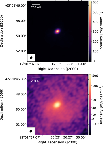
Figure 1. The continuum emission of BHR 71 at 356 GHz shown in linear scale (top) and symmetric logarithmic scale (bottom). For the bottom figure, the brightness is shown in logarithmic scale for  mJy beam−1, and in linear scale for
  . The synthetic beam is shown in the lower left corner. Table 2 lists the properties of the continuum source.
Download figure:
Standard image High-resolution imageTable 2. The Best-fitted Continuum Emission
| Parameter | Value |
|---|---|
| R.A. | 12h01m36 4988 ± 00001 4988 ± 00001 |
| Decl. | −65d08m493819 ± 00007 |
| Convolved size | |
| Semimajor axis FWHM | 521.3 ± 2.1 mas |
| Semiminor axis FWHM | 394.0 ± 1.3 mas |
| Position angle | 124 91 ± 048 91 ± 048 |
| Deconvolved size | |
| Semimajor axis FWHM | 349.5 ± 3.6 mas |
| Semiminor axis FWHM | 278.9 ± 2.7 mas |
| Position angle | 1137 ± 20 |
| Integrated flux | 1.129 ± 0.006 Jy |
| Peak flux | 586.9 ± 2.2 mJy beam−1 |
| Beam size | 039 × 027 (PA = 13125) |
Download table as: ASCIITypeset image
Dust emission can provide the dust mass if the dust emission is optically thin. Any optically thick matter, such as a compact disk, will make the derived mass an underestimation. The mass of optically thin dust can be evaluated with the following equation,
where Sν is the continuum flux density, d is the distance to BHR 71, κ356 GHz is the dust opacity at 356 GHz, 1.86 cm2 g−1, and Bν(356 GHz, Tdust) is the Planck function at 356 GHz given a temperature of Tdust. The assumption of a single dust temperature results in ∼10–50% uncertainty on the derived mass (Figure A.1 of Kauffmann et al. 2008). Thus, we use a mass-weighted temperature of 148 K (Equation 8 of Kauffmann et al. 2008) as the dust temperature for Equation (1). The derivation of the mass-weighted temperature assumes the density profile of a purely infalling envelope ( ; Ulrich 1976), the opacity of the dust covered with thin ice mantles at a gas density of 106 cm−3 (hereafter the OH5 dust, κν ∝ ν1.8; Ossenkopf & Henning 1994) and T(r) = 114 K evaluated at 70 au (035) from the Y17 model. The optically thin dust mass is 2.3
  ± 1.2
± 1.2  M⊙, suggesting a gas mass of 2.3 ± 0.01 M⊙ with a gas-to-dust ratio of 100. The error only represents the uncertainty of the flux measurement, whereas the systematic uncertainties from other origins, such as the dust opacity and calibration, are not included.
3.2. Molecular Emission
3.2.1. Intensity Maps
The intensity maps of HCN,  , CS, and H13CN emission (Figure 2) illustrate the structure of the outflows and the inner envelope within the central 12'', separated into the ranges of −5 km s−1 < v − vlsr < 0 km s−1 (blueshifted) and 0 km s−1 < v − vlsr < 5 km s−1 (redshifted). The source velocity is −4.45 km s−1, measured from the NH3 spectra in Bourke et al. (1997). While the emission peaks at the center of BHR 71 across a range of velocities (
 km s−1), the low-velocity (
 km s−1) emission also traces the morphology of outflows along the north–south direction. Here, we describe the red- and blueshifted velocity morphologies in detail.
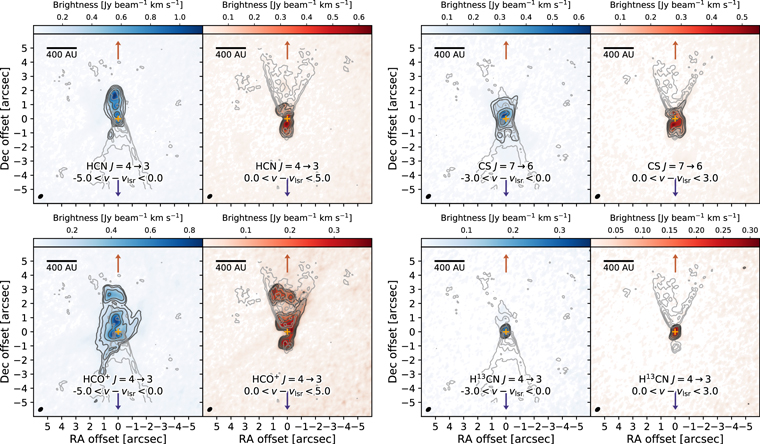
Figure 2. Moment 0 maps of the HCN  ,
, 
 , CS
, CS  , and H13CN
  lines, shown separately for blueshifted and redshifted velocities with respect to the source velocity. Orange plus signs indicate the position of the continuum source identified in Section 3.1, while the black ellipses indicate the beam sizes. For comparison with the CO outflows, the gray contours show the ALMA CO
  moment maps with a beam of 023 × 020, indicated by the white ellipse on top of the beam of the corresponding molecular lines. CO moments are calculated with the same velocity range as that of the corresponding molecular lines. Blue CO contours are separated linearly from 0.08 to 0.56 Jy beam−1 km s−1, while red CO contours are separated linearly from 0.11 to 0.42 Jy beam−1 km s−1. These maps only show the central 12'' of the entire observation, as regions outside of this area contain no significant emission. Contours show five equally separated levels in logarithmic scale from 2σ to their maximum values. There is very little emission at
  km s−1 for the CS
  and H13CN
  lines; therefore, we reduce the velocity range to better visualize the weak emission. Red and blue arrows indicate the large scale red- and blueshifted outflows (Bourke et al. 1997; Tobin et al. 2019).
Download figure:
Standard image High-resolution imageThe brightness of the HCN  line extends toward the north at the blueshifted velocities and toward the south at the redshifted velocities; this is opposite to the direction of the large-scale outflows observed in CO (Bourke et al. 1997; Parise et al. 2006b). The HCN emission is concentrated into a few compact features with a size of ∼05 or less, which will be further discussed in Section 7.
At redshifted velocities, the 
 emission resembles the shape of a triangular outflow cavity, similar to the outflow traced by CO (Tobin et al. 2019). In contrast, at blueshifted velocities, the emission becomes more extended than the morphology at the redshifted velocities, containing two filamentary structures at the west and south of BHR 71. A boxy feature with a size of 2'' × 3'' appears at 3'' north of BHR 71 at both blueshifted and redshifted velocities.
The CS  line also traces the morphology of the outflow cavities. At blueshifted velocities, the emission becomes more extended to the north and only traces the outflow cavity walls at the south; at redshifted velocities, the emission shows a similar morphology but reflects through the east–west plane, tracing the outflow cavity walls at the north and extending toward the south. The emission of
  and CS trace a shape that is similar to that of the outflow cavities.
The H13CN  emission has two peaks less than 05 away from the center of BHR 71, one at the north and one at the south. The morphology of H13CN emission is similar at blueshifted and redshifted velocities. As discussed in later sections (Section 5.2 and Appendix D), the emission of SO2 contaminates the H13CN
  line. The estimated brightness of this SO2 line is about one-third of the H13CN line, which dominates the intensity map shown in Figure 2. However, the morphology of another SO2 line at 356,755 MHz has a similar double-peaked morphology, suggesting the emission of both SO2 and H13CN may have the same origin. Overall, all four emission lines have morphologies more complex than a single peak, tracing structures along the outflow direction. Both CS and
  trace the outflow cavities, while HCN and H13CN appear as collections of compact features.
3.2.2. Velocity Maps
Figure 3 shows the first moment (the intensity-weighted velocity) maps of all four lines. The HCN, CS, and H13CN lines show redshifted emission at the south and blueshifted emission at the north, opposite to the kinematics of the large scale of CO outflows (Bourke et al. 1997; Parise et al. 2006b). However, the high-velocity emission appears in the north and south at redshifted and blueshifted velocities, respectively, consistent with the kinematics of the large-scale outflows (Figure 4).
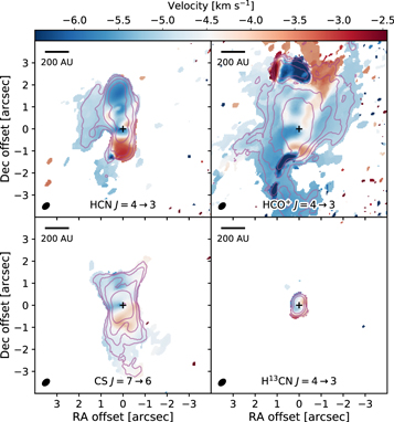
Figure 3. Moment 1 maps of the HCN  ,
, 
 , CS
, CS  , and H13CN
  lines shown together with the moment 0 maps in magenta contours, which show five equally separated levels in logarithmic scale from 2σ to their maximum values. From left to right, and top to bottom, the 2σ values are 0.02, 0.02, 0.02, and 0.01 Jy beam−1 km s−1, respectively; the maximum values are 1.47, 1.05, 0.93, and 0.62 Jy beam−1 km s−1, respectively. Both moment 0 and 1 maps are calculated from
  km s−1. Plus signs indicate the position of the continuum of BHR 71.
Download figure:
Standard image High-resolution image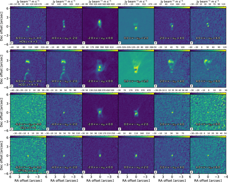
Figure 4. Channel maps of HCN  ,
, 
 , CS
, CS  , and H13CN
  from the top to bottom rows. Subset images show the moment 0 map calculated with the velocity ranges shown in the images, and each image has its own scaling to show a complete structure at each channel. The synthesized beam is shown at the lower left corner of each image.
Download figure:
Standard image High-resolution imageThe moment 1 map of the  emission shows a complex structure. The redshifted emission resides at the western side of BHR 71, while the blueshifted emission surrounds the source. Toward the south, a red-to-blue velocity gradient appears to align with the filamentary structure found in the intensity map. At the northern feature identified in the intensity map (Figure 2), a strong velocity gradient from blueshifted in the west to redshifted in the east coincides with this feature, along with the weak redshifted emission right next to the blueshifted component of this feature.
3.2.3. Channel Maps
Figure 4 shows the channel maps of all four lines, providing a detailed view of the velocity structure of these lines. For the HCN  line, we identify four compact features at low velocity, especially −4 km s−1 < v − vsource < 2 km s−1. We further discuss the origin of these HCN features in Section 7. The channel maps of the
 line show a similar morphology to the moment 0 map. The extended emission in the north disappears at low velocities, where more filamentary structure appears around the source. The CS
  line shows a single compact emission at most of the velocities except for the low velocities, where the emission exhibits an hourglass shape resembling that of the outflow cavities. The hourglass shape also appears in the low-velocity emission of HCN and
  . The converging ends of the outflow cavity extend ∼06–1'' perpendicular to the direction of outflows, corresponding to 120–200 au. Since these are optically thick transitions, the radius is an upper limit. Finally, the H13CN line maps show a single compact source at high velocity, consistent with the kinematics of the large-scale outflows, while two compact sources appear at low velocities with a separation of ∼05 (100 au). As shown in the moment 1 map of the H13CN
  line (Figure 3), the northern and southern sources have brighter emission at blueshifted and redshifted velocities, respectively, which shows the opposite kinematics as the high-velocity emission. As we pointed out in Section 3.2.1, a SO2 line contaminates the H13CN
  line, which also has a double-peaked morphology in the intensity map (Appendix D). However, zoom-in channel maps of these two lines (Figure 5) show different morphology variations as a function of velocity, suggesting that the observed morphology at the H13CN
  line is mostly due to H13CN. The redshifted part of the SO2 line peaks at the south, whereas the redshifted part of the H13CN
  line peaks at the north.
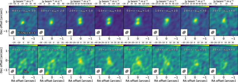
Figure 5. Zoomed-in channel maps of the SO2 line at 356,755.2 MHz and the H13CN  line. Each panel shows the moment 0 map within a 1 km s−1 interval from −4 km s−1 to 4 km s−1.
Download figure:
Standard image High-resolution image4. Infall Kinematics
We use four molecular lines, HCN,  , CS, and H13CN, to trace the infall kinematics in the envelope of BHR 71. The infall signature is best illustrated by the 1D line profiles. Here, we first characterize the observed line profiles, then present a radiative transfer model to constrain the underlying kinematics traced by these lines. The radiative transfer uses a 2D axisymmetric envelope model calculated in full 3D to include the effect of inclination.
4.1. The Infall Signature
We extract the spectra of HCN,  , CS, and H13CN lines from the region of continuum emission (052 × 039) in order to search for the redshifted absorption against the continuum, indicative of the infalling gas in the envelope in front of the source (Leung & Brown 1977; Zhou 1992; Choi et al. 1999; Di Francesco et al. 2001; Evans et al. 2005, 2015). The LOS toward the continuum source would have the deepest absorption as well as the least contamination from the outflows, making it the best position to search for the infall signature. We use the CASA specflux task to calculate the mean intensity, and fit the baseline for the second time. For each spectral window, a linear polynomial is fitted to the line-free channels visually selected from each spectral window (see the discussion in Section 5.1) in order to achieve a better baseline calibration.
Figure 6 shows the line profiles of HCN,  , CS, and H13CN targeted for measuring the infall kinematics. All four lines show blue asymmetric double-peaked profiles with the
 line having the greatest asymmetry among these four, followed by CS
  , HCN
, HCN  , and H13CN
  , whose two peaks have almost an equal intensity. Both the HCN
  and
and 
 lines show redshifted absorptions below the continuum, which is an unambiguous signature of infall. The absorption of the HCN
  line is narrower and has a greater redshift than that of the
 line. Within the absorption feature, if we take the midpoint of the velocities where the flux density is lower than the continuum as an estimate of the redshift of the absorption feature, the absorptions in the HCN
  and
and 
 lines center at 0.17 km s−1 and 0.14 km s−1, respectively. The CS and H13CN lines also show absorptions at their line centers, but not below the continuum flux. The HCN line profile has several narrow absorption features with decreases of ∼6 K, inconsistent with the hyperfine splitting of the HCN
  line. Therefore, the nature of these absorption features remains unclear. The FWHM of the line profiles excluding the absorption are 6.0 km s−1, 3.1 km s−1, 3.2 km s−1, and 4.1 km s−1, for the HCN
  ,
, 
 , CS
, CS  , and H13CN
  lines, respectively, showing that the HCN line is significantly broader than the other lines. The profile of the
  line best represents the infall signature as first proposed by Leung & Brown (1977), Zhou et al. (1993), and Di Francesco et al. (2001).
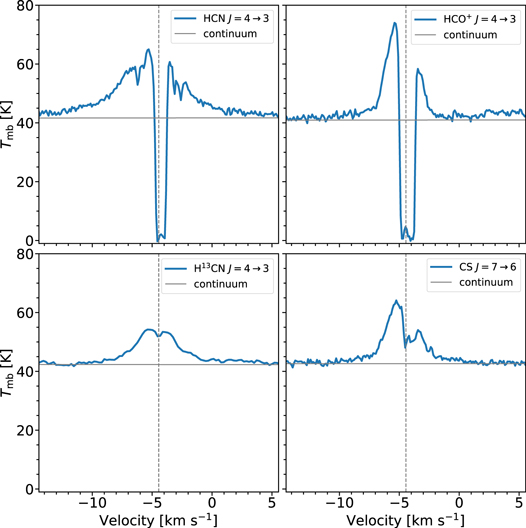
Figure 6. The spectra of HCN  ,
, 
 , CS
, CS  , and H13CN
  tracing the infalling envelope. The source velocity is −4.45 km s−1 (Bourke et al. 1997). The horizontal lines indicate the fitted continuum, while the vertical lines indicate the source velocity.
Download figure:
Standard image High-resolution imageThe absorption features seen in the  and HCN lines have a small peak at the bottom, where the envelope should absorb most of the emission. Because this small peak appears on top of a deep absorption, the origin of this peak must be in front of the dense envelope. Such emission could arise from the surface layer of the envelope heated by the interstellar radiation field.
4.2. Modeling the Infall
We successfully detect the infall signatures from our ALMA observations (Section 4.1). The redshifted absorption against the continuum provides strong evidence for the presence of infalling gas along the LOS. The absorption allows us to probe the velocity field and thus the age and rotation of the infalling envelope. To constrain the underlying kinematics, we model the line profiles using non-LTE radiative transfer in 3D to properly consider the absorption. By introducing the chemical abundance, a series of non-LTE radiative transfer calculations optimizes the 2D axisymmetric envelope model based on Y17 to reproduce the observations. The modeling focuses on the spectra toward the central continuum source, to minimize the contamination of outflows. However, given the moderate inclination of BHR 71 and the broad line profiles of the HCN  and H13CN
  lines, outflows may still contribute to the spectra at the beam toward the continuum source, especially the emission at velocities greater than ±2 km s−1. Thus, the radiative transfer modeling is mostly constrained by only the low-velocity emission, and aims to investigate how well an envelope model can explain the observed infall signature.
There are two types of inclination angles adopted in this study, one in the observer coordinates and another one in the model coordinates. Figure 7 shows the rotated BHR 71 system as viewed by observers. For characterizing models, we typical show quantities in the model coordinates and from θ = 0° to 90°; for comparisons with the observations, the model is viewed from θobs (130°). For the model, viewing from θ = 50° is equivalent to the view from θobs (130°) because of the symmetry of the envelope model with the outflows at the north–south direction.
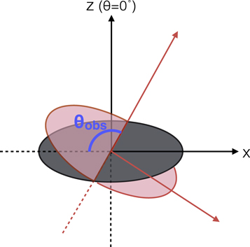
Figure 7. An illustration of a rotated system similar to the orientation of BHR 71. The y-axis is perpendicular to the figure. The black/gray system represents the spherical coordinates of the BHR 71 model with θ as the polar coordinates and the +z-axis as the rotation axis of the system. As viewed by observers from −x-axis, BHR 71 is rotated away from the line of sight (−x) by 130°, illustrated by the red/pink system. The inclination angle viewed by observers is denoted as θobs.
Download figure:
Standard image High-resolution image4.2.1. Updating the Continuum Model
Y17 presented a TSC envelope with the geometry of outflow cavities. The prescription of the model is 2D axisymmetric, but the calculations are carried out in 3D to model the inclination of the rotation axis. We discovered a numerical error in calculating the density around the centrifugal radius (13 au in the Y17 model), causing an underestimation of the density around the centrifugal radius. The updated radial density profile (Figure 8) has a clear density peak at the centrifugal radius similar to the analytical solution of the disk in Ulrich (1976) and Cassen & Moosman (1981). Dominated by the envelope, the radial brightness profile extracted from the synthetic image at 160 μm still agrees with the Herschel observation after correcting this numerical error, which determines the age of the TSC model (Yang et al. 2017).
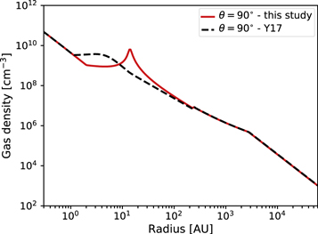
Figure 8. Radial density profile of the updated continuum model of BHR 71 (red) compared with the profile shown in Y17 (dashed black). Only the density profiles along the midplane of the envelope are shown here. The envelope age is 36,000 yr.
Download figure:
Standard image High-resolution image4.2.2. The Radiative Transfer Model
We perform radiative transfer calculations to constrain the kinematics of the infalling envelope. Figure 9 illustrates the workflow for modeling the infall signature. Using hyperion (Robitaille 2011), Y17 constrains the parameters of the 2D axisymmetric TSC envelope model with the far-infrared Herschel spectra and the archival data of BHR 71, which provides the gas density, velocity vector fields, and dust temperature (Tdust) as functions of radius r and polar angle θ. The temperatures of gas and dust are in equilibrium when the gas density is greater than 104–105 cm−3 (Young et al. 2004), where the Y17 model suggests ∼104 au for both the radius of ngas = 104 cm−3 and the radius of Tdust = 10 K. Thus, we set the gas temperature to the dust temperature when Tdust > 10 K, and then apply an external heating correction when Tdust < 10 K, following the model in Young et al. (2004).
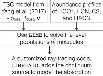
Figure 9. Workflow of modeling the infall profile. The ρgas, Tdust, and  represent the gas density, dust temperature, and velocity vector, respectively.
Download figure:
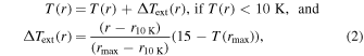
Standard image High-resolution imageAn external heating correction applies for the cells with temperatures lower than 10 K. The correction is a linear function that increases with the radius such that the temperature at the edge of the envelope becomes 15 K, described as
where rmax is the envelope outer radius of 0.315 pc, and r10 K is the radius where the temperature becomes less than 10 K. A typical r10 K is ∼10,000 au, similar to the values derived from self-consistent radiative transfer calculations of dense cores (Young et al. 2004). Figure 10 shows the radial temperature profiles before and after applying the external heating. While the external heating correction has no significant impact on the synthetic line profile, we apply the external heating as described in Equation (2) to the model, for consistency.
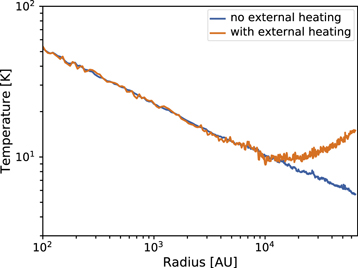
Figure 10. Radial temperature profiles along the midplanes of the envelopes with cavities. The same external heating correction also prescribes to the entire envelope. The orange line shows the profile with the external heating, while the blue line shows the profile without the external heating.
Download figure:
Standard image High-resolution imageWith all other parameters taken from the best-fitting dust model, the abundances of the molecules are the main free parameters in this study. The main parameters for the Y17 model of the TSC envelope are sound speed, rotational speed, and age, which are 0.37 km s−1, 5  rad s−1, and 34,000 yr, respectively. In Section 4.2.4, we investigate the impact of different abundance profiles on the observed infall signature. The following paragraphs describe the procedures of calculating the synthetic line profiles. We employ the Line Modeling Engine (lime; Brinch & Hogerheijde 2010) to obtain the molecular level populations and then post-process the model with a customized ray-tracing code to include a central continuum source. lime iteratively solves the equation of radiation transport assuming non-local thermodynamical equilibrium (non-LTE), and produces image cubes for the specified molecular transitions.
Gridding is critical to ensure a realistic representation of the input model. lime automatically determines the gridding based on the temperature and density profiles. However, discontinuities, such as the cavities, in models often lead to unrealistic cell structure in the gridding. Thus, we run lime with the density profile without the cavities to ensure a robust gridding. We assume a zero abundance in the outflow cavities, as these molecular lines show little emission along the outflows at high velocities. Molecules around the cavity walls may contribute to the observed spectrum. Modeling the emission from outflow cavity walls requires an accurate model for the kinematics and abundance, which has been elusive and is beyond the scope of this study. The synthetic continuum emission may be slightly overestimated—but negligibly so, due to the low density in the cavities.
We set up the lime model with 50,000 grid points distributed in a spherical envelope of 30,000 au according to the density profile. The minimum spatial scale is 1 au. While using more grid points will reduce the potential clustering, where the grid points show an unusual overdensity at a localized region, we find no difference in the synthetic line profiles calculated with 50,000 grid points versus 500,000 grid points. We also set the maximum radius in lime smaller than the maximum radius in the model, 64,973 au, to better sample the high-density regions. Extending the model to the full size of the envelope has negligible effect on the synthetic line profiles. lime uses sink points at the surface of the model to collect the emitting rays for imaging. Because we post-process the derived level populations output to add the central continuum source, the number of the sink points is irrelevant.
Simulating the absorption against the continuum requires a central continuum source, which is beyond the capability of lime. Therefore, we developed a ray-tracing package, lime-aid (LIME-Additional Intensity Decoder), to include continuum sources in our model, taking the level populations from lime along with the temperature, density, velocity, and abundance to calculate the LOS image cubes. The code itself is a derivative of the Cosmic Lyα Transfer code (colt; Smith et al. 2015), with the Monte Carlo scattering procedures replaced by ray-tracing. The code also runs natively on unstructured data (Smith et al. 2017), i.e., the Voronoi tessellation of points, which is efficiently and robustly constructed with the Computational Geometry Algorithms Library (The CGAL Project 2018). Appendix A provides a detailed description of lime-aid.
4.2.3. The Kinematics of Infalling Envelopes
In a TSC envelope, matter rotating infalls onto the midplane of the envelope. Figure 11 illustrates the velocity in spherical coordinates along three different polar angles. The velocity vector is defined with respect to the origin of the model, the center of the envelope (i.e., negative in vr indicates infall). Along the midplane of the envelope (θ = 90°), the centrifugal force becomes significant at small radii compared to other θ. Thus, the radial velocity decreases most slowly along the midplane of the envelope, where the azimuthal velocity increases most rapidly as the radius decreases. In the polar direction (θ = 0°), gas infalls without rotation; therefore, the radial velocity increases the fastest as the radius decreases, while the polar and azimuthal velocities remain zero. The TSC envelope does not follow the dynamical evolution within the centrifugal radius, where a disk may form. Thus, a Keplerian disk does not evolve from the TSC model.
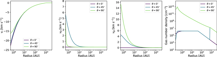
Figure 11. The radial, polar, and azimuthal velocity profiles, as well as the gas density as a function of radius from the best-fitted TSC envelope (from left to right), which is the same model in Y17 with an age of 12,000 yr instead. The dust sublimation at high temperature leads to the decrease of density at the innermost region along the θ = 0° and 45°. The velocity profiles along three different polar angles are shown, where θ = 0° is face-on and θ = 90° is edge-on. The negative velocity for vr indicates that the gas is moving toward the center.
Download figure:
Standard image High-resolution image4.2.4. Constraining the Abundance Profile
The molecular abundance is a strong function of temperature and density in the protostellar envelope. At the outer envelope, the molecules become photodissociated by the external radiation field. As the radius decreases, molecules become abundant due to the shielding from dust. However, molecules may freeze onto the dust grains at low temperature and high density. The freeze-out timescale for molecules is inversely proportional to the gas density and the squared root of the temperature (Lee et al. 2004). In the envelope, the density increases much more rapidly than the temperature as the radius decreases. Thus, molecules become increasingly frozen-out toward smaller radii. When the temperature is higher than the evaporation temperature of the molecules, the abundance increases again as the molecules are released from the ices. Jørgensen et al. (2004) use a "drop function," a constant abundance along with a region of lower abundance, to simplify the freeze-out process for modeling the CO line profiles. Here, we start with the simple drop function for the abundance profile, to try to fit the observed infall profiles.
The drop function depends on four parameters: the evaporation temperature (Tevap), the depletion density (ndepl), the density at which the molecule depletes (X0), and the depleted abundance (Xdepl). We test the feasibility of the drop function on the 
 , whose profile resembles a typical infall signature, i.e., a redshifted absorption against the continuum along with a clear blue-asymmetric double-peaked profile. The desorption temperature of CO determines the production of
  ; therefore, we set the evaporation temperatures of
  to either a typical temperature of 20 K (Lee et al. 2004) or to a slightly higher temperature of 30 K (Jørgensen et al. 2002). Additionally, we add a destruction temperature of 100 K, where water becomes evaporated and destroys
  (Jørgensen et al. 2013), acting as an inner cutoff radius of the abundance profile. We explore the parameter space using 54 models with 10−10 ≤ X0 ≤ 10−7, 10−11 ≤ Xdepl ≤ 10−8, 105.5 ≤ ndepl (cm−3) ≤ 108, and Tevap = 20, 30 K, distributed linearly in logarithmic scale. Figure 12 shows the spectra of all 54 synthetic line profiles compared with the observation. The models with the drop function result in too much emission at high velocities, when the synthetic spectra agree with the absorption feature. The synthetic spectra underestimate the high-velocity wings when matching the peaks of the observations. Our experiments suggest that the drop function fails to provide the required flexibility to model the high-resolution ALMA spectra. Evans et al. (2005) also found that a simple step function requires unlikely combinations of parameters to fit the observations of B335.
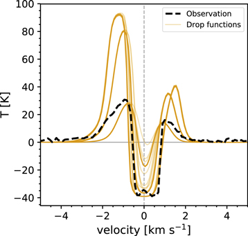
Figure 12. Observed 
 line profile along with the spectra modeled with the drop function abundance. A total of 54 models are presented here. The lack of agreement with the observations suggests the need for a more complex abundance profile than the drop function.
Download figure:
Standard image High-resolution imageTo overcome the limitation of the drop function abundance, we construct a parameterized abundance profile that resembles the features in the chemophysical modeling (Lee et al. 2004). Such a profile has the flexibility to reproduce not only the abundance of  but also HCN, CS, and H13CN. Here, we use
  as an example to describe the effect of each parameter (Table 3).
  is a daughter molecule of CO and
  formed by the reaction, described as

Thus, the freeze-out of CO dominates the abundance of  when the temperature is lower than the evaporation temperature of CO, 20 K (Lee et al. 2004). When the temperature becomes higher than the evaporation temperature of CO, the abundance of
  increases. The low abundance of
  due to the low ionization in the high-density inner regions makes the abundance in the evaporation zone lower than the abundance in the outer envelope. Instead of a sudden drop in the abundance in the "drop function," we set the abundance proportional to r2 in the freeze-out zone until CO becomes evaporated at the inner high-temperature region. The high CO abundance enhances the production of
  and other carbon-bearing molecules. When the temperature becomes higher than 100 K, water (a major destroyer of
  ) sublimates, reducing the abundance of
  . For other molecules, such as HCN and CS, the gas-phase chemical equilibrium may also reduce their abundance at high temperature. Toward the edge of the envelope, the external radiation field photodissociates the
  . Thus, we introduce a decrease of the abundance at the outer radius as r−2. Finally, we set the abundance at the inner evaporation zone (Xevap) lower than the outer region, which has the maximum abundance (Xout). The value of Xout is not necessarily greater than that of Xevap for other molecules. Figure 13 illustrates the constructed abundance profiles and the corresponding parameters.
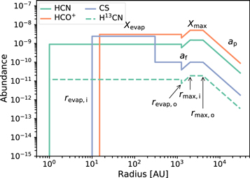
Figure 13. Best-fitted parameterized abundance profiles for HCN,  , CS, and H13CN. The H13CN abundance is one-third of the abundance of HCN.
Download figure:
Standard image High-resolution imageTable 3. Parameters of the Abundance Profiles (Figure 13)
| Parameter | Description |

|
HCN | CS | H13CN |
|---|---|---|---|---|---|
| Xout | Maximum abundance | 5.0 
|
8.0 
|
1.0 
|
2.7 
|

|
Abundance of the evaporation zone | 2.0 
|
1.0 
|
2.5 
|
3.3 
|
| rmax, i | Inner radius of the maximum abundance region | 1000 au | 1000 au | 1000 au | 1000 au |
| rmax, o | Outer radius of the maximum abundance region | 1500 au | 1200 au | 1500 au | 1200 au |

|
Inner radius of the evaporation zone | 50 au | 1 au | 10 au | 1 au |

|
Outer radius of the evaporation zone | Set to 1250 au | |||
| af | Power-law index of the freeze-out zone | Set to 2.0 | |||

|
Power-law index of the outer decreasing region dominated by photodissociation | Set to −2.0 | |||
Download table as: ASCIITypeset image
The chemical evolution of CO also controls the abundance profiles of HCN and CS. When CO freezes onto dust grains, HCN and CS abundances are also reduced. Once CO becomes evaporated, the gas-phase production of HCN and CS increases (Lee et al. 2004). For HCN, the gas-phase abundance eventually becomes unsustainable for chemical equilibrium, such that its abundance decreases in the higher-temperature region (i.e., inner radius). Lee et al. (2004) find three peaks in the abundance profile of HCN in the protostellar stage, corresponding to the evaporation of CO, HCN, and CN; however, our experiment suggests that the abundance with only one evaporation zone can reproduce the observations. The abundance of H13CN follows the abundance of HCN divided by the isotope ratio of 77 (Wilson & Rood 1994). CS has two peaks in its abundance profile. The first one occurs where CO is evaporated, while the second one occurs at an inner radius where CS (which has a higher evaporation temperature) is evaporated. The abundance of CS remains high at the inner radius, where most of the oxygen still freezes onto dust grains as atomic oxygen and water. Thus, sulfur atoms tend to stay in CS rather than SO, which would be preferred if oxygen abundance increases. At large radii, CS has a low abundance, due to the destruction by UV photons.
Our experiments with the CS abundance profile suggest a need for two evaporation zones to describe the observations. With only one evaporation zone, the synthetic spectrum typically overestimates the absorption. Our experiments show that only decreasing the abundance in the evaporation zone can effectively reduce the absorption, but it also reduces emission at the same time (Figure 14). As Lee et al. (2004) demonstrate, the abundance of CS has two peaks inside the region where the temperature is greater than the CO evaporation temperature. Thus, we set up two evaporation zones, corresponding to 20 K for CO and 35 K for CS for the abundance of CS.
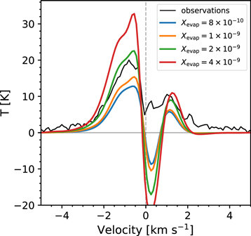
Figure 14. Synthetic CS line profiles as a function of the abundance in the evaporation zone.
Download figure:
Standard image High-resolution imageIn general, the properties of the evaporation zone (abundance, inner and outer radii) dominate the resulting synthetic spectra, while the combination with the outer abundance profile has secondary effects to tune the line profile. To constrain the abundance profile, we set the initial parameters with insights into the chemical modeling found in Lee et al. (2004). Next, we manually search for the best-fitting abundance profile while exploring the effect of each parameter. During the search, the evaporation radius is fixed to 1000 au, where the temperature is ∼20 K in the midplane of the envelope. The slopes of freeze-out and photodissociation are fixed to 2 and −2, to reduce the number of degrees of freedom.
4.3. The Best-fitting Model
Figure 15 shows the best-fitting infall profiles sampled with the same uv-coverage of our ALMA observation using the CASA tasks simobserve and simanalyze. We take the best-fitted parameters from Y17 as the initial guess of the model, and iterate the abundance profiles and ages to find the best-fitting models. The lime-aid program includes the central continuum source according to the 2D continuum fitted from the line-free channel in each spectral window, instead of an averaged continuum over all spectral windows. Table 4 lists the properties of the continuum emission fitted at each molecular line.
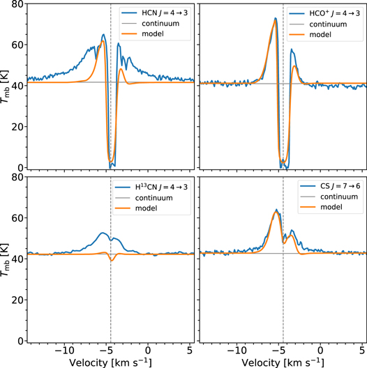
Figure 15. Synthetic spectra of HCN  ,
, 
 , CS
, CS  , and HCN
  in orange, along with the observed line profile in blue, and the continuum fitted from the observations in gray. Emission of identified COMs is subtracted for the spectra of
 and H13CN
  lines, which makes the spectra slightly different than the spectra shown in Figure 6.
Download figure:
Standard image High-resolution imageTable 4. The Observed and Fitted Continuum Emission at Each Molecular Line
| Line | Size | PA | Observed Fcont | Fitted Fcont |
|---|---|---|---|---|
| ('') | (°) | (Jy) | (Jy) | |
HCN 
|
0.31 ± 0.03 × 0.27 ± 0.03 | 97 ± 39 | 1.11 | 1.12 |
 
|
0.37 ± 0.03 × 0.28 ± 0.03 | 106 ± 17 | 1.16 | 1.20 |
CS 
|
0.32 ± 0.03 × 0.27 ± 0.03 | 99 ± 22 | 1.03 | 1.06 |
H13CN 
|
0.33 ± 0.02 × 0.27 ± 0.02 | 118 ± 15 | 1.04 | 1.05 |
Download table as: ASCIITypeset image
Sampling the synthetic image cube with the ALMA uv-coverage is the last step of modeling. Due to the imperfect uv-coverage of the ALMA observations, the resulting spectra after simulating the ALMA visibility show a systematic decrease of 2 K on the continuum, and the decrease becomes as high as 4 K at the peak of the line, which is consistent with some contribution from the extended line emission and the compact continuum source. Thus, we tune the input continuum flux densities to match the observed continuum. Table 4 lists the best-fitted continuum fluxes.
As we will further discuss in Section 5.2, the emission of acetone (CH3COCH3) and deuterated methanol (CH2DOH) contributes to the line profile of the 
 line, and the emission of SO2 contaminates the H13CN
  line profile; thus, we subtract the modeled emission of those molecules from the observed line profiles, for an accurate comparison against the models. We also summarize the effect of cavities and inclination in Appendix B. Figure 13 shows the best-fitting abundance profiles of
  , HCN, CS, and H13CN with the best-fitting parameters listed in Table 3. Moreover, Table 5 lists other important parameters of the model.
Table 5. Important Parameters of the Model of BHR 71
| Parameter | Description | Value |
|---|---|---|
| tage | Age of the protostellar system after the start of collapse | 12,000 yra |

|
Effective sound speed of the envelope including the turbulent velocity | 0.37 km s−1 |

|
Turbulence velocity | 0.34 km s−1 |
| Ω◦ | Initial angular speed of the cloud | 2.5 × 10⁻¹³ rad s−1 |
| Renv | Envelope outer radius | 0.315 pc |
| Rcen | Centrifugal radius | 0.6 aua |
| θcav | Cavity opening angle | 20° |
| θobs | Inclination angle of the protostar | 130° |
Notes. Please see Yang et al. (2017) for detailed prescription of the composite model of BHR 71, especially the treatment of the disk.
aThe age is reduced to fit the molecular lines. The centrifugal radius is also changed correspondingly.Download table as: ASCIITypeset image
4.3.1. The Implied Protostellar Age
The parameterized abundance profile provides a great flexibility to model the infall signature. However, the velocities where the line profile peaks are less variable than the changes in the abundance profile. We take the averaged difference of the peak velocities,  =
=  +
+ , as an indicator of the goodness of the fitting for the peak positions. Figure 16 shows the
  map of a grid of models for the
 line where only the chemical abundance profile varies. This grid of models has an age of 36,000 yr, the age derived in Y17. While the abundance parameters vary by more than two orders of magnitude,
  only decreases from 1.1 to 0.5 km s−1. Moreover, the model with lower abundances produces a better match to the peak positions, because the line profile becomes much flatter and only the low-velocity emission appears. This model fails to reproduce the intensity of the observed infall signatures, but with an younger age of 12,000 yr, the
  becomes 0.2 km s−1 for the
 line without compromising of the intensity. Thus, the age parameter is more effective at changing the velocities where the line profile peaks, making the peak positions a strong diagnostic of age.
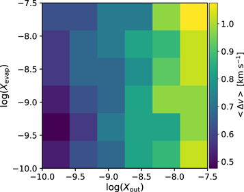
Figure 16. The squared difference of the peak velocities, (Δv)2, from a grid of models of the 
 line. The definition of Δv is described in Section 4.3.1. All models have an age of 36,000 yr, but with different evaporation abundances (Xevap) and maximum abundances (Xout) as indicated in the figure. In comparison, the Δv becomes 0.4 km s−1 for the best-fitting model of the
 line with an age of 12,000 yr.
Download figure:
Standard image High-resolution imageA TSC model with an age of 36,000 yr produces infall signatures that peak at higher velocities than that of the observations. The  and HCN lines require an age less than 20,000 yr, while the CS line requires an age of 12,000 yr. The envelope with a younger age still agrees with the radial brightness profile of BHR 71, because the χ2 value essentially levels off below 36,000 yr (Yang et al. 2017). To further characterize the uncertainty of the model-derived age, we run a grid of models whose ages range from 10,000 to 15,000 yr with 1000 yr increments, and compare the velocities of the peak positions against the CS line profile, which demands a younger age. The minimum averaged velocity difference occurs at the age of 12,000 yr with
  km s−1. The difference becomes 0.10 km s−1 and 0.11 km s−1 for the ages of 13,000 and 11,000 yr. If we take the spectral resolution, 0.1 km s−1 as a threshold for the uncertainty, the derived age is 12,000 ± 2000 yr.
With the updated age, the total infalling gas mass becomes 0.15 ± 0.04  , instead of 0.43
  from the age best-fitted with the continuum SED, which is only 6.5% of the gas mass derived from the continuum. If we consider the optically thick dust emission, the discrepancy becomes even greater. Such discrepancy hints that the infall rate may have been higher in the past.
4.3.2. Turbulence Velocity
We iteratively test different abundance profiles for each molecule to find the best-fitting model. While the synthetic profiles qualitatively reproduce the observations, the modeled absorption feature has always been slightly broader than the observations, where changing the abundance profile has little effect. Thus, we decrease the turbulence velocity from 0.34 km s−1, derived in Y17 based on the ammonia observations by Bourke et al. (1995), to 0.25 km s−1 (Figure 17). In comparison, Y17 derive an effective sound speed of 0.37 km s−1, contributed by a thermal velocity dispersion with T = 13 K derived by Bourke et al. (1995) and a turbulence velocity of 0.34 km s−1. The discrepancy in the turbulence velocity is similar to the uncertainty in the line width measurements of the ammonia observations, 0.1 km s−1.
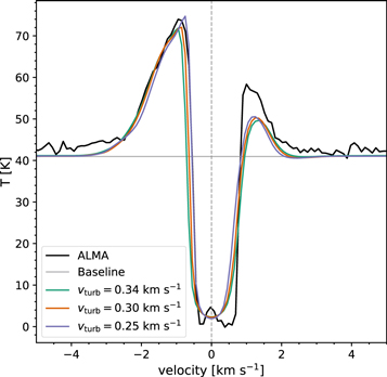
Figure 17. The synthetic line profiles of the 
 line with three different turbulence velocities. A vturb of 0.34 km s−1 is the same as the one used by Y17, but a vturb of 0.25 km s−1 reproduces the line profiles reasonably well.
Download figure:
Standard image High-resolution image4.3.3. The Compact Continuum Emission
The shortcomings of the infalling envelope model at the inner ∼100 au and the COMs emission suggest a compact rotational structure with a radius of ∼50 au, just below the spatial resolution of our observations. To test the possibility of a compact source, we compare the observed uv-visibility with our envelope model. The continuum visibility shows a peak at small uv-distance and a slowly declining tail at the long uv-distance (Figure 18). The compact continuum source fitted from the image (Figure 1) has FWHMs of 035 × 028, which correspond to Gaussian widths of 312 kλ and 391 kλ in uv-visibility, respectively. A Gaussian fit to the observed uv-visibility at uv-distance greater than 150 kλ finds a Gaussian with a width of 332 kλ, which is consistent with the compact continuum source (Figure 18). Our envelope model qualitatively agrees with the visibility after subtracting the compact source. Both models of the envelope and the compact continuum source underestimate the visibility at large uv-distance, suggesting a more compact unresolved source within the continuum shown in Figure 1.
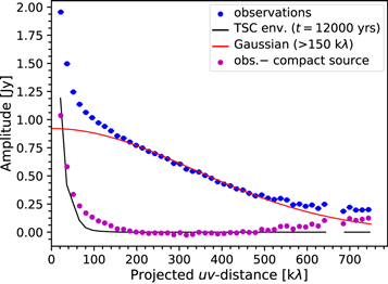
Figure 18. The uv-visibility of the observed continuum compared with the TSC envelope model of an age of 12,000 yr. Weighted visibility is binned into 50 bins, where the mean and uncertainty are calculated. Observations and envelope model are shown in blue and black, respectively. Red line indicates a Gaussian fit to the visibility with uv-distance >150 kλ. The Gaussian is centered at zero with an amplitude of 0.92 J7 and a Gaussian width of 332 kλ. Magenta dots show the visibility after subtracting the fitted Gaussian component.
Download figure:
Standard image High-resolution image4.3.4. Shortcomings of the Model
Our models reproduce the line profiles of HCN  (except for the high velocity wings),
 , and CS
  lines, but fail to reproduce the H13CN
  line. The TSC model has its limitations. For instance, the model ignores the angular momentum transportation within the centrifugal radius, where a disk should be forming. Thus, the rotation velocity within the centrifugal radius remains constant instead of approaching Keplerian under the TSC model (see Figure 11). The Larson–Penston type of collapse is an alternative to the TSC model. Hunter (1977) describes the similarity solution after the core formation following a Larson–Penston collapse (see also Saigo & Hanawa 1998). With a higher infall velocity, a Larson–Penston collapse results in a greater peak separation than that of the observations (Zhou 1992). Adopting a Larson–Penston collapse in our 3D radiative transfer modeling is challenging because most of the models are in 1D (e.g., Saigo & Hanawa 1998). Numerical simulations are another alternative to the TSC model (e.g., Gong & Ostriker 2015; Tomida et al. 2015). However, most of the numerical models are not optimized to a certain source. Fully characterizing the numerical models require exploration of parameter space and realizations along the dynamical evolution, which are beyond the scope of this study.
The High-velocity Wings of the HCN Line—The best-fitting HCN model has high abundance at the region as close as 1 au to the central protostar, driven by the broad peak at the blueshifted velocity and the chemical modeling (Lee et al. 2004). However, line width increases rather moderately, indicating that the inner evaporation radius is ill-constrained. None of the models under our setup can reproduce the broad high-velocity emission. Outflows may contribute to the high-velocity HCN emission; however, the high-velocity emission is mostly concentrated at the center (Figure 4) instead of following the morphology of the outflows. Thus, the high-velocity emission suggests an unexpected structure at the inner envelope, possibly an unresolved disk (see Section 6.3).
The H13CN Line—To model the profile of the H13CN  , we start with scaling down the HCN abundance by 77, the isotope ratio of 12C/13C (Wilson & Rood 1994). However, this abundance profile produces a very weak line profile, inconsistent with the observation. Next, we test different 12C/13C ratios and find the best fit for a ratio of 3 for the model best-fitting the observation, which has a ratio of 3 for 12C/13C. While a 12C/13C ratio of 3 is highly unlikely, such a high ratio suggests that the H13CN
  line requires additional structures on top of our model. Given the compact morphology of the H13CN emission (Figure 2), a highly concentrated structure at the center of BHR 71 may reproduce the observations. The model for another protostar, B335, also shows a similar discrepancy between the models and the H13CN
  line (Evans et al. 2015). The possible underlying structure remains unknown, but future observations of the emission of COMs that are concentrated in the central region may provide insights to this inconsistency. Aside from from the overall strength of the H13CN
  line, our model predicts a significant absorption, whereas our observations show only a self-absorption of ∼5 K. Typically, increasing the exponent of the power law for the outer photodissociation region reduces the absorption, but in the case of H13CN, where we drastically decrease the abundance at the outer envelope (Figure 13), the absorption still largely disagrees with the observation. The best-fitting CS abundance has a large evaporation zone ranging from 10 to 400 au. To match the observed absorption feature, we not only need to make the abundance decrease more rapidly at the photodissociation region but also to reduce Xout.
Comparison with the Single-dish Observations—Figure 19 shows the synthetic spectrum of the 
 line using the best-fitting model of
  compared with the archival APEX observation, which has a 233 beam. While the synthetic emission has a strength comparable to the observation, the line profile is significantly different. The observation shows significant blue asymmetry between the two peaks, whereas the model suggests an equal-strength double-peaked profile. Given that our model is optimized for the ALMA observations, which is only sensitive to the structure smaller than 3'', we do not optimize our model for the single disk observation. However, a comparable strength of the double-peaked profile suggests that the TSC envelope cannot fully describe the structure of BHR 71. From the Herschel/SPIRE 500 μm image, the envelope of BHR 71 exhibits an asymmetric structure elongated along the northwest–southeast direction (e.g., Yang et al. 2017; Tobin et al. 2019). If the foreground is more opaque than the TSC model predicts, the absorption would be shifted toward the velocities where it is observed. Also, at larger scales, the envelope deviates significantly from spherical symmetry (Tobin et al. 2010). Observations that measure the chemical abundance of
  (e.g., the observation of H13CO+) and probe the intermediate scales between the single dish data and our ALMA observation may revise our model to fit the data at both low and high resolutions.
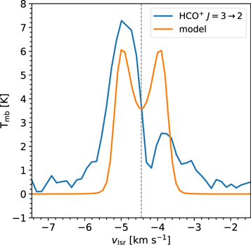
Figure 19. Synthetic 
 line profile (orange) compared with the archival APEX observation (blue). The model is the same best-fitted model for the
 line extracted from a 233 circular aperture without any beam correction.
Download figure:
Standard image High-resolution image5. Complex Organic Molecules
The bandwidths of our observations (∼200 km s−1 and ∼400 km s−1) allow us to not only measure infall indicators but also survey the emission of complex molecules at similar frequencies. Throughout the dynamical evolution of dense cores from prestellar to protostellar, the chemical state of the molecular gas evolves as the material experiences variations in both density and temperature, which determines the available chemical reactions. Over the last decade, observations have revealed a new class of protostars that exhibit rich spectra of COMs from a warm inner region of their envelopes (T ≳ 100 K), the so-called "hot corinos" (Ceccarelli 2004; Ceccarelli et al. 2007). The formation of COMs depends on the environments, including temperature, density, and the sites of formation, which are constantly modified by the dynamical evolution of the star formation (Garrod et al. 2008; Aikawa 2013). While ALMA is revolutionizing the discovery of hot corinos (e.g., The ALMA Protostellar Interferometric Line Survey; Jørgensen et al. 2016), the link between the physics of star formation and the hot corino chemistry is relatively unknown. In this section, we analyze the emission of molecules that do not trace the infall in the ALMA spectra extracted from the continuum size (052 × 039) smoothed to 1 km s−1 to optimize the line detectability.
5.1. The Spectra of COMs
The entire spectra of our ALMA observations shows many emission lines apart from the emission that probes the infall (Figure 20). On average, these emission mostly come from the central 050 ± 013 × 021 ± 009 (100 au × 42 au) region, while several emission lines shows extensions in the north–south direction (∼1'' in size), consistent with higher abundances of COMs due to the increased temperature in the outflow cavity. The mean line width of these emission is 4.5 ± 2.5 km s−1 with a median width of 3.7 km s−1; however, the widths of some lines may be overestimated due to the blending with other lines. Appendix C describes the fitting and properties of these emission lines.
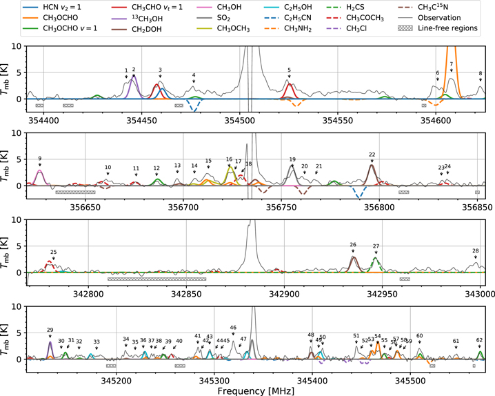
Figure 20. The 1D spectra of BHR 71 with molecular species labeled. Confirmed identifications are shown as positive spectra, while the tentative species are shown as negative spectra. Observed spectra are smoothed with an 1D Gaussian kernel that has a FWHM of 1 km s−1 to achieve a higher S/N on the weak emission. The numbers of the identified features are consistent with the line number shown in Table 9. Line 46 is identified as the emission of CH3OD, which is not included in the database queried by xclass, hence not modeled. Horizontal bars beneath the spectra indicate the line-free regions selected for baseline fitting and calibration.
Download figure:
Standard image High-resolution image5.2. Line Identification
We use splatalogue15 and xclass (Möller et al. 2017) to identify the lines seen in Figure 20. The spectroscopic data are taken from the Cologne Database of Molecular Spectroscopy (Müller et al. 2001, 2005; Endres et al. 2016) and the Jet Propulsion Laboratory (Pickett et al. 1998). Here, we list only the references that cover the frequencies relevant to this study. For HCN v2 = 1, the data were taken from Thorwirth et al. (2003). For CH3OH, the data were taken from Xu et al. (2008); for CH2DOH, the data were taken from Pearson et al. (2012); for 13CH3OH, the data were taken from Xu & Lovas (1997). For CH3OCHO, the data were taken from Ilyushin et al. (2009), which includes the data from Plummer et al. (1984), Oesterling et al. (1999), Carvajal et al. (2007), Maeda et al. (2008a). For CH3CHO, the data were taken from Kleiner et al. (1996). For CH3OCH3, the data were taken from Endres et al. (2009). For CH3COCH3, the data were taken from Groner et al. (2002). For CH3Cl, the data were taken from Wlodarczak et al. (1986). For CH3C15N, the data were taken from Müller et al. (2009) together with the data from Pearson & Mueller (1996). For CH3NH2, the data were taken from Kréglewski & Wlodarczak (1992). For gauche-C2H5OH, the data were taken from Pearson et al. (2008) together with the data from Pearson et al. (1996). For CH3CH2CN, the data were compiled from Pearson et al. (1994) and Brauer et al. (2009). For SO2, the data were taken from Müller & Brünken (2005) with additional data from Lovas (1985), Helminger & De Lucia (1985), and Belov et al. (1998). Finally, for H2CS, the data were taken from Müller et al. (2019) together with the data from Johnson et al. (1971) and Maeda et al. (2008b).
To confirm identifications, we observe the following guidelines in Snyder et al. (2005)
- 1.Rest frequency: The identified transition has to have its rest frequency measured in-laboratory or calculated to have an uncertainty at least on the order of 1 part in 10 million, corresponding to ∼0.04 MHz for our data.
- 2.Frequency agreement: To assign a robust identification from the selected possible transitions, the assigned transition needs to agree with the observed line within the half width at half maximum of the line.
- 3.Relative intensity: After a transition is assigned, the relative strengths of all other transitions for the identified molecules need to match with the observation.
For each line, we search the transitions with a maximum upper energy of 1000 K, and test if the corresponding species produces spectra consistent with the observations using xclass, assuming a typical model of an excitation temperature of 100 K and a line width of 3.5 km s−1. The xclass program considers the optical depths of both dust and molecules. The best-fitting envelope model (Section 4.2.1) provides an estimate of the dust column density. The emission of each molecule does not interact with those of others. Table 6 lists the results of the line identification. The emission of CH3OD is identified with the results in Anderson et al. (1988) instead of the modeling with xclass.
Table 6. Line Identification
| Formula | Name | Frequency (MHz) | Transitiona | Einstein-Ab | Eu (K) | Line No. |
|---|---|---|---|---|---|---|
| Confirmed identifications | ||||||
| CH3OH | Methanol | 356626.667(0.016) | [J, K] = [23, 4] → [22, 5] | 8.041(−5) | 728 | 9 |
| 13CH3OH | Methanol | 345132.599(0.05) | [4, 0, 4] → [3, 1, 3] | 8.239(−5) | 36 | 29 |
| 13CH3OH | Methanol | 354445.95(0.05) | [4, 1, 3] → [3, 0, 3] | 1.274(−4) | 44 | 2 |
| CH2DOH | Methanol | 356697.9372(0.0099) | [9, 2, 8] → [9, 0, 9] | 3.536(−6) | 133 | 13 |
| CH2DOH | Methanol | 356796.1421(0.0034) | [8, 6, 3] → [7, 6, 2] | 6.277(−5) | 234 | 22 |
| CH2DOH | Methanol | 356796.1421(0.0034) | [8, 6, 2] → [7, 6, 1] | 6.277(−5) | 234 | 22 |
| CH2DOH | Methanol | 345398.9037(0.0112) | [16, 2, 14] → [15, 3, 13] | 4.275(−5) | 310 | 48 |
| CH2DOH | Methanol | 342935.6452(0.0118) | [17, 2, 16] → [17, 1, 17] | 1.227(−4) | 343 | 26 |
| CH3ODc | Methanol | 345319.587(0.359) | [J, K, parity] = [8, 2, −] → [8, 1, +] | 8.1 (μ2Σ S) | 100 | 46 |
| CH3OCHO | Methyl formate | 345465.3445(0.0023) | [16, 13, 4] → [16, 12, 5], Sym = E | 2.513(−5) | 192 | 54 |
| CH3OCHO | Methyl formate | 354608.0913(0.003) | [33, 0, 33] → [32, 1, 32] | 1.097(−4) | 293 | 7 |
| CH3OCHO | Methyl formate | 354608.0919(0.003) | [33, 1, 33] → [32, 1, 32] | 6.792(−4) | 293 | 7 |
| CH3OCHO | Methyl formate | 354608.0923(0.003) | [33, 0, 33] → [32, 0, 32] | 6.792(−4) | 293 | 7 |
| CH3OCHO | Methyl formate | 354608.0928(0.003) | [33, 1, 33] → [32, 0, 32] | 1.097(−4) | 293 | 7 |
| CH3OCHO | Methyl formate | 345461.011(0.1) | [28, 13, 15] → [27, 13, 14], Sym = E | 4.94(−4) | 352 | 53 |
| CH3OCHO | Methyl formate | 345486.602(0.1) | [28, 13, 16] → [27, 13, 15], Sym = E | 4.941(−4) | 352 | 58 |
| CH3OCHO | Methyl formate | 356711.841(0.1) | [29, 17, 12] → [28, 17, 11] | 4.561(−4) | 448 | 15 |
| CH3OCHO | Methyl formate | 356711.841(0.1) | [29, 17, 13] → [28, 17, 11] | 4.561(−4) | 448 | 15 |
| CH3OCHO v = 1 | Methyl formate | 345162.544(0.1) | [11, 8, 3] → [10, 7, 3], Sym = E | 7.091(−5) | 269 | 32 |
| CH3OCHO v = 1 | Methyl formate | 345148.04(0.1) | [28, 6, 23] → [27, 6, 22], Sym = A | 5.947(−4) | 452 | 31 |
| CH3OCHO v = 1 | Methyl formate | 356686.906(0.1) | [29, 6, 24] → [28, 6, 23] | 6.584(−4) | 469 | 12 |
| CH3OCHO v = 1 | Methyl formate | 345473.217(0.1) | [28, 9, 19] → [27, 9, 18], Sym = E | 5.626(−4) | 481 | 55 |
| CH3OCHO v = 1 | Methyl formate | 345510.004(0.1) | [28, 9, 20] → [27, 9, 19], Sym = A | 5.635(−4) | 481 | 60 |
| CH3OCHO v = 1 | Methyl formate | 345571.314(0.1) | [27, 5, 22] → [26, 5, 21], Sym = E | 6.055(−4) | 481 | 61 |
| CH3OCHO v = 1 | Methyl formate | 345248.21(0.1) | [28, 10, 19] → [27, 10, 18], Sym = E | 5.481(−4) | 493 | 39 |
| CH3COCH3 | Acetone | 342780.0361(0.0357) | [17, 17, 0] → [16, 16, 1] | 1.85(−3) | 147 | 25 |
| CH3COCH3 | Acetone | 342780.0345(0.0357) | [17, 17, 1] → [16, 16, 0] | 1.85(−3) | 147 | 25 |
| CH3COCH3 | Acetone | 345256.0368(0.0368) | [18, 15, 4] → [17, 14, 3] | 1.287(−3) | 151 | 40 |
| CH3COCH3 | Acetone | 345305.3651(0.0367) | [18, 15, 3] → [17, 14, 4] | 1.288(−3) | 151 | 45 |
| CH3COCH3 | Acetone | 356675.1969(0.0814) | [19, 13, 6] → [18, 12, 7] | 6.123(−4) | 158 | 11 |
| CH3COCH3 | Acetone | 356658.4123(0.0187) | [27, 10, 17] → [26, 11, 16], Sym = EA | 1.215(−3) | 275 | 10 |
| CH3COCH3 | Acetone | 356658.4780(0.0187) | [27, 11, 17] → [26, 10, 16], Sym = EA | 1.215(−3) | 275 | 10 |
| CH3COCH3 | Acetone | 356658.5351(0.0184) | [27, 10, 17] → [26, 11, 16], Sym = AE | 1.215(−3) | 275 | 10 |
| CH3COCH3 | Acetone | 356658.6016(0.0184) | [27, 11, 17] → [26, 10, 16], Sym = AE | 1.215(−3) | 275 | 10 |
| CH3COCH3 | Acetone | 356729.9828(0.0153) | [27, 10, 17] → [26, 11, 16], Sym = EE | 1.215(−3) | 275 | 18 |
| CH3OCH3 | Dimethyl ether | 356705.204(0.004) | [8, 4, 4] → [7, 3, 5], Sym = AE | 9.249(−5) | 55 | 14 |
| CH3OCH3 | Dimethyl ether | 356712.951(0.002) | [8, 4, 5] → [7, 3, 5], Sym = EE | 6.255(−5) | 55 | 15 |
| CH3OCH3 | Dimethyl ether | 356724.457(0.003) | [8, 4, 4] → [7, 3, 5], Sym = AA | 2.095(−4) | 55 | 16 |
| CH3OCH3 | Dimethyl ether | 356724.864(0.003) | [8, 4, 5] → [7, 3, 5], Sym = AE | 1.17(−4) | 55 | 16 |
| C2H5OH | gauche-Ethanol | 345173.9493(0.0112) | [J,  , ,  , vt] = [7, 7, 1(0), 0] → [6, 6, 1(0), 1]d , vt] = [7, 7, 1(0), 0] → [6, 6, 1(0), 1]d
|
2.515(−4) | 140 | 33 |
| C2H5OH | gauche-Ethanol | 345229.238(0.05) | [J,  , ,  , vt] = [21, 1, 21, 0] → [20, 1, 20, 0] , vt] = [21, 1, 21, 0] → [20, 1, 20, 0] |
3.728(−4) | 242 | 36 |
| C2H5OH | gauche-Ethanol | 345295.3553(0.0022) | [J,  , ,  , vt] = [21, 1, 21, 1] → [20, 1, 20, 1] , vt] = [21, 1, 21, 1] → [20, 1, 20, 1] |
3.731(−4) | 246 | 43 |
| C2H5OH | gauche-Ethanol | 345408.1651(0.0022) | [J,  , ,  , vt] = [21, 0, 21, 1] → [20, 0, 20, 1] , vt] = [21, 0, 21, 1] → [20, 0, 20, 1] |
3.743(−4) | 246 | 49/50 |
| SO2 | Sulfur dioxide | 356755.1899(0.0014) | [10, 4, 6] → [10, 3, 7] | 3.281(−4) | 90 | 19 |

|
Thioformaldehyde | 342946.4239(0.0500) | [10, 0, 10] → [9, 0, 9] | 6.08(−4) | 91 | 27 |
| HCN v2 = 1 | Hydrogen cyanide | 354460.4346(0.0007) | J = 4 
|
1.869(−3) | 1067 | 3 |
| Tentative identifications | ||||||
| CH3CHO vt = 1 | Acetaldehyde | 354522.7114(0.1995) | [6, 6, 1] → [7, 5, 3] | 3.184(−6) | 304 | 5 |
| CH3CHO vt = 1 | Acetaldehyde | 354457.6646(0.0409) | [18, 2, 16] → [17, 2, 15] | 1.585(−3) | 375 | 3 |
| CH3C15N | Methyl cyanide | 356761.0470(0.002) | [J, K] = [20, 1] → [19, 1] | 3.962(−3) | 187 | 20 |
| CH3CH2CN | Ethyl cyanide | 354476.6596(0.0015) | [40, 3, 38] → [39, 3, 37] | 3.767(−3) | 361 | 4 |
| CH3Cl | Methyl chloride | 345408.9874(0.0023) | [J, K, F] = [13, 3, 12.5] → [12, 3, 11.5] | 7.764(−4) | 183 | 49/50 |
Notes.
aThe typical quantum numbers are listed as [J, ,
,  ] unless specified.
bThe number in the parentheses indicates the power of 10 (e.g., 8.041(−5) represents 8.041
] unless specified.
bThe number in the parentheses indicates the power of 10 (e.g., 8.041(−5) represents 8.041  ).
cAnderson et al. (1988).
dTwo degenerate transitions occur for
).
cAnderson et al. (1988).
dTwo degenerate transitions occur for  =
=  and
and  .
.
Download table as: ASCIITypeset image
Some species—such as methyl formate (both ground state and excited state), dimethyl ether, acetone, methanol, and ethanol—have multiple lines detected in our observations, allowing us to further constrain their excitation temperatures and column densities. With xclass, LTE radiative transfer calculations produce synthetic spectra that are optimized to the observations. We further exclude possible optically thick emission from the optimization, based on the line profile, such as significant deviations from Gaussianity and absorption. The properties of methyl formate (both ground state and excited state) and dimethyl ether are fitted simultaneously due to blending between their spectra. Other species, such as acetone, deuterated methanol (CH2DOH), and ethanol, are fitted separately. Table 7 lists the fitted excitation temperatures and column densities for selected species. For methanol and its isotopologues, only CH2DOH has sufficient detections to determine its properties; thus, the fitting of column densities of CH3OH and 13CH3OH assumes the excitation temperature of CH2DOH. Given the distribution of the fitted temperatures, we take 100 K as the typical temperature to fit the column densities for other identified species, also shown in Table 7.
Table 7. The Abundance of Identified COMs
| Species | Formula | No. of Identified Lines | Tex (K) | Column Density (cm−2) | Abundance to 
|
|---|---|---|---|---|---|
| Species with fitted temperatures and column densities | |||||
| Methanol | CH2DOH vt = 0 | 3 | 100 | 6.9 
|
4.1 
|
| Methanol | 13CH3OH vt = 0 | 2 | 100a | 1.3 
|
7.6 
|
| Methanol | CH3OH vt = 0 | 1 | 100a | 2.4 
|
1.4 
|
| Methyl formate | CH3OCHO v = 0 | 4 | 100 | 4.4 
|
2.6 
|
Methyl formate ( ) ) |
CH3OCHO vt = 1 | 7 | 150 | 3.7 
|
2.2 
|
| Acetone | CH3COCH3 v = 0 | 5 | 130 | 9.7 
|
5.7 
|
| Dimethyl ether | CH3OCH3 v = 0 | 3 | 60 | 1.0 
|
5.9 
|
| gauche-Ethanol | C2H5OH v = 0 | 5 | 260 | 1.3 
|
7.6 
|
| Species with fitted column densities assuming Tex = 100 K | |||||
| Sulfur dioxide | SO2 v = 0 | 1 | 100b | 2.7 
|
1.6 
|
| Thioformaldehyde | H2CS v = 0 | 1 | 100b | 9.9 
|
5.8 
|
| Hydrogen cyanide | HCN v2 = 1 | 1 | 100b | 4.0 
|
2.4 
|
Notes. These column density are fitted with an excitation temperature of 100 K. The gas column density within a 05 radius beam is 1.7  cm−2, calculated from the best-fitting envelope model.
Download table as: ASCIITypeset image
Figure 20 shows the best-fitting spectra of the identified COMs along with the spectra of the tentatively identified COMs, which only serves as a consistency test, as our observation cannot confirm the identifications of those species. The lines excluded from the optimization due to suspected high optical depth, such as Lines 7 and 54, have significant deviation from the modeled spectra. While methylamine is not identified, its spectra show some agreement with the observations (see the discussion in Appendix E), which requires future line surveys to confirm. Our identification of COMs and their compact morphology at <1'' region indicate that BHR 71 has a hot corino. Aside from the COMs, ALMA ACA observations detect the emission of carbon-chain molecules (Ł. Tychoniec 2020, in preparation), suggesting that BHR 71 may have different degrees of complex chemistry at different spatial scales.
6. Addressing the Shortcomings of the Infall Model
6.1. An Observational Test of the Best-fitting Infall Kinematics
While the infall signature toward the continuum source provides the least contaminated signature to constrain the underlying infall kinematics, the variations of infall signatures across the envelope will further assess the effects of rotation and abundance profile. Figure 21 shows the PV diagrams of the observations and the best-fitting models. Aside from the H13CN  line, the modeled morphology at the zero offset agrees with the observations relatively well compared with the offset positions, since the models are constrained at the central position. Overall, our models have emission more spatially extended than the observations, suggesting a denser inner region or a lower density at the outer region than the model predicts. Since the envelope model has been constrained with the far-infrared SED, which mainly probes the outer envelope, a denser inner region is a more plausible scenario. Under the TSC framework, a higher density at the inner region requires a younger age or a higher effective sound speed, resulting in a more compact density peak or a higher rotation speed at the inner region, in turn leading to a larger centrifugal radius. However, the uncertainty in the chemical abundance should be characterized before any quantitative comparison.
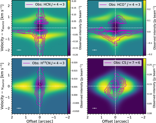
Figure 21. The PV diagrams of the best-fitting envelope models (images) compared with the observed PV diagrams (magenta contours), extracted with a slice across the midplane of the envelope (east–west). Contour levels increase linearly from 0.05 to 0.26, 0.05 to 0.55, 0.02 to 0.17, and 0.05 to 0.28 for the HCN  ,
, 
 , H13CN
  , and CS
  lines, respectively. The synthetic PV diagrams are convolved with the spectral and spatial resolutions of the observations, which are indicated as white error bars.
Download figure:
Standard image High-resolution imageThe variation of the infall signature across the midplane of the envelope presents another way to investigate the infall kinematics. Here, we focus on the 
 line best-fitted by our model. The blue asymmetric double-peaked profile only appears within the inner 05 region, whereas only a single blue peak exists beyond the inner 05 region (Figure 22, solid lines). In the observations, the strength of the red peak increases from east to west, as is expected due to the rotation; however, the observations show a much greater difference than our model. The widths of the two peaks in the infall signature also change from east to west, especially the blue peak, which becomes broader at the 05 offset and narrower at the −05 offset. Except for pointings toward the center and −05, the model disagrees with the observations. The synthetic profile shows a higher intensity when the pointing is displaced by 05 from the center due to the reduction of the optical depth. As we move further away from the center along the midplane, the decrease of molecular abundance starts to dominate the behavior of the synthetic profile, resulting in a gradual decrease in the overall intensity.
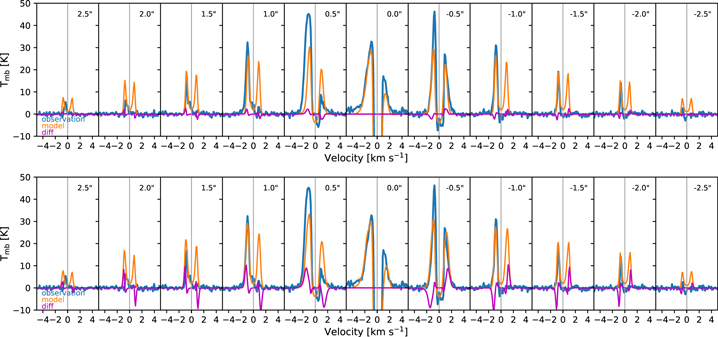
Figure 22. Two grids of the 
 line profiles extracted with 05 × 05 box regions along the midplane of the envelope (east–west). The top panel shows the best-fitting model. The bottom panel shows the same model with a higher Ω of 10−12 rad s−1, whose line profiles peak at slightly higher velocity. Those regions offset from the center ranging from 25 to −25 in RA. Observation is shown in blue. Models are shown in orange. Magenta lines show the difference in the synthetic spectra to the opposite side of the offset (i.e., the line for 05 is the difference of profiles toward 05 and −05).
Download figure:
Standard image High-resolution imageThe comparison between our models and the observations highlights two issues. First, our TSC envelope model underestimates the variation of the redshifted peak across the inner 05 region due to the rotation. As discussed in previous paragraphs, a larger centrifugal radius may reduce the disagreement in the PV diagrams between the observations and the models (Figure 21), suggesting a higher rotation at the inner region. In fact, a TSC envelope with twice the best-fitting rotation speed, 5  rad s−1, leads to a greater asymmetry for the
  line profiles at one side of the midplane than another; for the
  line profile at the 05 offset, the peak of the difference (magenta line in Figure 22) becomes ∼10 K. The observation shows a difference of ∼20 K, suggesting a much faster rotation at the inner 05 region. However, the linewidth variation as a function of the offset cannot be obviously explained by a higher rotation.
Second, the  model fails to explain the disappearance of the redshifted emission beyond the inner 05 region. Moreover, the synthetic infall signatures overestimate the intensity at off-center positions for all four lines, suggesting more complex abundance profiles. The temperature gradient in the envelope governs the degree of asymmetry between the blueshifted and redshifted peaks, and also produces the redshifted emission as long as the warm gas in the foreground of the infalling envelope falls within the LOS. If we increase the depletion in the freeze-out zone of the abundance profile to fit the redshifted peaks, both the blueshifted and redshifted peaks would have the same sudden disappearance beyond the inner 05 region, which is not observed. The lack of redshifted emission may also explain the significant blue asymmetry in the
 line observed by APEX (Figure 19), while our model predicts an equal-strength double-peaked profile.
A model with a higher rotation speed of 10−12 rad s−1 results in a moderately brighter red peak at the −05 position, whereas the brightness of the red peak remains the same at the 05 position (Figure 22). The blue peak shows a similar behavior with a moderate brightness at the 05 position but the same brightness at the −05 position. Thus, it is unlikely that the behavior of the infall signatures within the inner 05 region is due to a higher rotation speed of the TSC model. A single Gaussian line shifted toward blue and red at the 05 and −05 positions, respectively, with the self-absorption at the source velocity could be consistent with the observations. Such a model would have a greater velocity shift than that of the TSC model, suggesting a higher rotation. Perhaps the higher rotation only occurs at the inner part of the envelope.
Figure 11 shows that the TSC model underestimates the rotation speed within the centrifugal radius. However, the observations show a higher rotation out to ∼100 au, which cannot be reproduced by the envelope model. A model with an older age would have a higher rotation as well as a larger centrifugal radius—indicating a larger disk, as our analyses hint. In contrast, the molecular line profiles require an age as young as 12,000 yr (Section 4.3.1). Resolving this issue requires a model that consistently describes the kinematics of both the envelope and the disk, as well as the observations targeting the embedded disk, such as the observations of C18O.
6.2. A Compact Rotational Structure Traced by COMs
Figure 23 shows the moment 1 maps of a selection of unblended COM emission, showing a velocity gradient in the west–east direction from blueshifted to redshifted, consistent with the velocity gradient seen in the emission of C18O (Tobin et al. 2019). Two of the COM emission lines, 13CH3OH at 354608.0 MHz and CH3OCHO at 345132.5 MHz, show the velocity gradient with high S/N, allowing further analyses with PV diagrams (Figure 24).
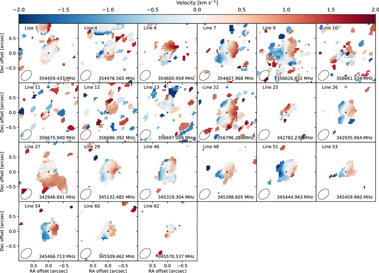
Figure 23. The moment 1 maps of the unblended COM emission, calculated with a 4 km s−1 window centered at the source velocity.
Download figure:
Standard image High-resolution image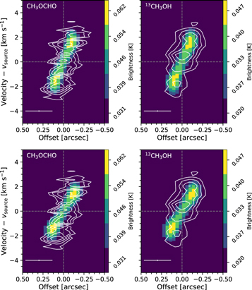
Figure 24. The PV diagrams of the emission of 13C-methanol and methyl formate (white contours) along with the synthetic PV diagrams of Keplerian disks (colored images) with a power-law radial brightness profile (top) and a uniform brightness (bottom). The PV slice is perpendicular to the outflows. The color bar shows the brightness of the modeled images, which are normalized to the maximum brightness of the observed PV diagrams. Ticks of the color bar indicate the contour values of the observed PV diagrams.
Download figure:
Standard image High-resolution imageThe emission of COMs better traces the kinematics at the inner region, as COMs only become abundant in the gas phase at T > 100 K; therefore, the emission only comes from the inner envelope, where a disk may be forming. To investigate the kinematics probed by COMs, we construct the PV diagrams along a slice perpendicular to the outflow direction, north to south (Bourke et al. 1997; Parise et al. 2006b), minimizing the contamination from the outflows. Assuming that the emission of COMs is optically thin due to their low column density, the PV diagrams of 13CH3OH and CH3OCHO allow us to qualitatively constrain the rotational kinematics.
The PV diagrams are first tested against a simple model of a Keplerian rotating disk. In an ideal case, a Keplerian disk would result in blueshifted velocities only at one side of the disk and redshifted velocities only at the other side; however, with a finite spatial resolution, the emission becomes smeared out at the low velocities; therefore, low velocities emission may appear at either side of the source. The emission of a Keplerian disk at any east–west offset from the center, b, can be written as
where θ is the angle between the LOS toward the source and the LOS according to b with respect to the source itself, R is the outer radius of the disk, and θincl is the inclination angle of the disk, 130°. The central mass, M, is set to the total infall mass inferred from our envelope model, 0.15  , and the line width, Δv, is assumed to be 1 km s−1. To match the spatial and spectral resolutions of the observations, a 2D Gaussian kernel is applied to the emission of the Keplerian disk.
The maximum velocity in the PV diagram determines the inner radius of the disk, 15 au, while the maximum spatial extent constrains the outer radius of the disk, 50 au. Next, we test two models of the radial brightness temperature profile, a constant brightness temperature throughout the disk, and a power-law profile, which represents the decrease of density toward outer radius. The disk is likely to be optically thick; however, to qualitatively test the Keplerian disk against our observations we assume the power-law profile has included the effect of optical depth. A more realistic model would have two power-law profiles jointed at a certain radius, representing the transition from optically thick to optically thin. However, such model has more parameters, requiring a better spatial resolution than that of our observations. For a qualitative comparison, the power-law profile is set to r−2, while Salyk et al. (2011) found a power-law slope of −1 to −3 using the two power-law model. Figure 24 shows the synthetic PV diagrams along with the observations, calculated with Equation (4) independent from the modeling of the infalling envelope. The two representative models show PV diagrams similar to the observations, suggesting that a Keplerian disk may contribute to the rotation signatures seen in the emission of COMs. Between the two brightness profiles, the power-law profile leads to the emission peaked at a lower velocity, better reproducing the observations. Although this comparison suggests a Keplerian would reproduce the PV diagrams of COMs, the minor difference between the PV diagrams of the two profiles highlights the need for high-resolution observations to characterize the nature of this rotation signature.
6.3. The Origin of the High-velocity Emission in the HCN and  CN Lines: Disks or Outflows?

While the infall model reproduces most of the ALMA observations, it fails to match the high-velocity wings in the HCN  line and greatly underestimates the H13CN
  line. The compact morphology of the H13CN
  line and the high apparent H13CN/HCN ratio suggest a compact optically thick structure at the center of BHR 71, which could be an unresolved disk motivated by the rotation observed in the emission of COMs (Section 6.2). A compact disk may produce the high-velocity emission observed in the HCN
  and H13CN
  lines; however, outflows may contribute to the high-velocity emission as well. The morphology of outflows (Figure 2) and the moderate inclination angle indicate that the LOS toward the central continuum source includes the outflows. To investigate possible origins of the high-velocity emission, we first test the possibility of an unresolved disk; we then discuss the cases for a disk and outflows.
According to Equation (4), the emission of a Keplerian disk shows a symmetric double-peaked profile (Figure 25). The disk emission is calculated separately from the infalling envelope, resulting in the lack of absorption at the source velocity. We start from a power-law radial brightness profile with the disk suggested from the COMs emission (rmin = 15 au and rmax = 50 au; Section 6.2), and vary the slope of the power-law profile to reproduce the observations. The optimization is done by eye. With a disk from 15 to 50 au, the model only produces emission up to ±3 km s−1 regardless of the power-law profile, whereas the observed profiles extend to velocities up to ±10 km s−1. Matching the wings of the HCN line requires an inner radius of 0.5 au. While a disk extending from 0.5 to 50 au reproduces the high-velocity wings for the HCN and H13CN lines reasonably well, the model overestimates the low-velocity emission of the HCN line. A smaller outer radius of 20 au would reduce the low-velocity emission, producing a better fit to the HCN line.
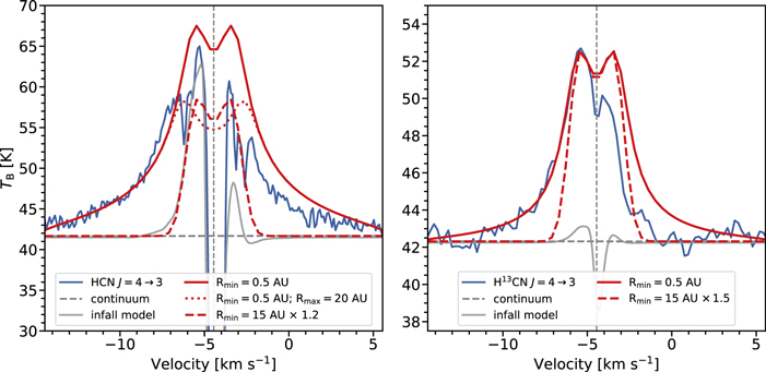
Figure 25. Spectra of the HCN  and H13CN
  lines (blue) along with the synthetic spectra of the infalling envelope (gray) and the Keplerian disk models, including a disk from 15 to 50 au (red dashed), a disk from 0.5 to 50 au (red solid), and a disk from 0.5 to 20 au (red dotted). Models with a disk from 15 to 50 au are scaled from the profiles listed in Equation (5) by 1.2 and 1.5 for the HCN and H13CN lines, respectively.
Download figure:
Standard image High-resolution imageWhile Keplerian disks produce the line profiles consistent with the observations, the underlying best-matched radial brightness temperature profiles are rather unphysical. The best-matched brightness profiles can be written as
Both profiles have unphysically high temperatures at 0.5 au, 103–104 K, and low temperatures at 50 au, 8–14 K, suggesting that a Keplerian disk may not be the origin of the high-velocity emission.
Outflows also produce high-velocity emission. At an inclination angle of 130°, the LOS toward the center is likely to includes some outflowing gas. However, confirming the contribution from outflows will require future models that combine the kinematics of both the infalling envelope and outflows.
7. Peculiar Kinematics of the HCN Compact Features
The channel maps of the HCN  emission reveal four compact features, labeled as N3, N2, N1, and S1 from north to south, peaking at 0.5–1.5 km s−1 relative to the source velocity, located along the outflow direction. Table 8 lists the sizes of these features fitted with a 2D Gaussian profile. Interestingly, if we focus on ±2 km s−1 around the source velocity, the three northern features peak at the blueshifted velocity, while the southern feature peaks at the redshifted velocity, an opposite kinematics to that of the outflow probed by CO (Bourke et al. 1997; Parise et al. 2006b). At velocities greater than 4 km s−1, the HCN emission only appears in the south at the blueshifted velocity and in the north at the redshifted velocity, following the kinematics of the outflows. N2 and N3 also appear in the CO observation with a similar resolution as that of HCN (M. Dunham 2020, private communication) in the same velocity range (Figure 26). At low velocity, the PV diagram along the outflow direction shows a triangular shape in these features, most significantly at N2 and N3.
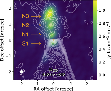
Figure 26. Moment 0 map of the HCN emission shown as an image with the moment 0 of the CO  emission plotted as contours (M. Dunham 2020, private communication). Both moments are calculated from −5 to 0 km s−1. Shown at the bottom left corner, the solid ellipse indicates the beam size of the CO observation, while the the greater ellipse outline indicates the beam size of the HCN observation.
Download figure:
Standard image High-resolution image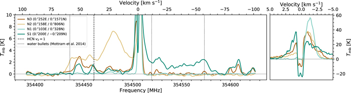
Figure 27. Left: full spectra of the four HCN features extracted from the fitted 2D Gaussian sources (Table 8). Velocities of the water bullets measured by Mottram et al. (2014) are shown in dotted lines, while the rest frequency of the HCN v = 2  line is shown in dashed line. Right: spectra of the same four HCN features, shown only around the line centroid of the HCN
  line.
line.
Download figure:
Standard image High-resolution imageTable 8. Source Fitting of the HCN Features Identified in Figure 26
| Name | R.A. | Decl. | FWHMs (mas) | PA |
|---|---|---|---|---|
| N3 | 12h01m3654 |
−65d08m4781 |
82 ± 3 × 59 ± 2 | 1548 ± 42 |
| N2 | 12h01m3652 |
−65d08m4858 |
66 ± 1 × 50 ± 1 | 1632 ± 22 |
| N1 | 12h01m3652 |
−65d08m4905 |
57 ± 2 × 49 ± 2 | 1455 ± 91 |
| S1 | 12h01m3650 |
−65d08m4959 |
52 ± 1 × 39 ± 1 | 978 ± 19 |
Download table as: ASCIITypeset image
We propose two scenarios for those features that have kinematics opposite to the outflows and small (∼1 km s−1) velocity shifts. The HCN features may be part of the outflows. The emission of the redshifted outflow can appear as blueshifted if the outflow opening angle is large enough to have parts of the outflow at the front side of the envelope. With an outflow opening angle of 225 measured at 10'' from the protostar using CO observations (Tobin et al. 2019) and an inclination angle of 130° (Yang et al. 2017) from the Y17 model, the projected positions of the HCN features are consistent with the region where the outflow extends in front of the plane of sky at high inclination, supporting this scenario (Figure 28). The outflow opening angle is defined as the angle between the rotation axis and the edge of the outflow cavity at 10,000 au (Yang et al. 2017), and the outflow cavity is assumed to have z ∝ ϖ1.5. However, if shocks lead to the excitation of those HCN features, we expect to observe a broad spectral feature from the shocked gas that is blueshifted for N1, N2, and N3, and redshifted for S1. Only N2 and S1 have broad features in their spectra, but the features appear at the velocity opposite to the one we expect (Figure 27).
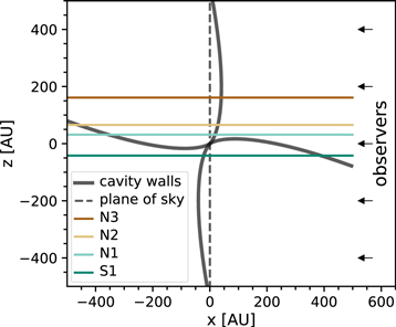
Figure 28. Illustration of the outflow cavity (black thick solid line) and the plane of sky (black dashed line) along with the lines of sight of the HCN features (colored lines), assuming an outflow opening angle of 225 (Tobin et al. 2019) and an inclination angle of 130° (Yang et al. 2017). The opposite kinematics would occur where the cavity walls appear at the opposite side to the majority of the outflow cavities with respect to the plane of sky (i.e., the northern redshifted outflow has parts of its cavity wall in front of the plane of sky).
Download figure:
Standard image High-resolution imageThe blueshifted infalling gas behind the outflow cavity can also result in the small blueshifted emission in the redshifted outflow. The best-fitting model of the infall profile has velocities similar to the velocity offset of those HCN features; however, the model also predicts more redshifted emission, which disagrees with the observation, and the model does not include the kinematics of the outflows. In this case, we expect to see a broad spectral feature at the redshifted velocity for N1, N2, and N3, which is consistent with the spectra of N2. Future high-resolution observations for probing the excitation mechanism of these HCN features, such as SiO tracing the shocked gas, may reveal the nature of the peculiar kinematics.
A compact feature also appears at high velocity. An offset compact emission peaks at ∼354,480 MHz (∼22 km s−1), if the source velocity of −4.45 km s−1 is assumed, in the spectrum centered on the HCN  line, extending over a wide range of frequencies (Figure 29). Measured by the CASA imfit task, this compact high-velocity emission peaks at 12h01m3653 and −65d08m4842 with a size of 054 × 047. Only seen offset from the center, the broad line profile is unlikely to be emitted by COMs. Shock-excited HCN
  v = 0 and v2 = 1 lines may contribute to the broad features extending toward high velocities. A velocity offset of 22 km s−1 to the HCN
  v = 0 and v2 = 1 lines would agree with the observations, and shocks would broaden the linewidth. Comparing to the HCN features defined at low blueshifted velocities, this high redshifted velocity compact feature peaks in between N2 and N3 and much closer to N2, suggesting that the same physical structure may contribute to the emission at both the low blueshift velocity and the high redshift velocity.
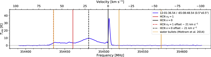
Figure 29. Spectrum of the high-velocity compact feature in the spectral cube centered on the HCN  line extracted from a 05 × 05 region. This feature is identified at ∼354,480 MHz. The black solid and dashed lines indicate the rest frequencies of the HCN
  v = 0 and v2 = 1 lines, respectively, while the red solid and dashed lines show the same two transitions shifted by −21 km s−1 to match the broad peak at 21 km s−1. The orange lines indicate the velocities of the water bullets identified by Kristensen et al. (2012) and Mottram et al. (2014).
Download figure:
Standard image High-resolution imageAcross the entire velocity range, high-velocity broad emission appears at both redshifted and blueshifted velocities, occurring at +09 and −04 to the continuum source (Figure 30, right). Kristensen et al. (2012) identify high-velocity "bullets," narrow offset features, from the water  emission, where Mottram et al. (2014) isolate the bullets at −57.4, −11.8, and 59.0 km s−1. The spectra of S1 and N3 as well as the PV diagrams along the outflows show emission peaks around −57.4 km s−1, but the observations cannot confirm other bullets. However, the spectra of the HCN compact features show broad emission over the velocities of the water bullets; thus, the high-velocity bullets may also present in our observations.
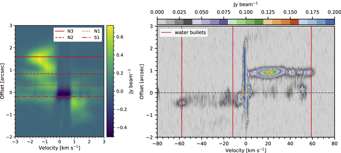
Figure 30. Left: the position–velocity diagram extracted along the HCN features. The horizontal lines indicate the locations of the HCN features. Right: the position–velocity diagram extracted from the same slice as the left figure shown in the full velocity range. The vertical lines indicate the velocities of the water bullets identified by Kristensen et al. (2012) and Mottram et al. (2014).
Download figure:
Standard image High-resolution image8. Conclusions
Using a 03 beam of ALMA, we successfully observe redshifted absorption against the continuum toward BHR 71 from the spectra of the 
 and HCN
  lines, which is an unambiguous signature of infall. The spectra of CS
  and H13CN
  also show redshifted self-absorption.
To constrain the underlying infall kinematics, we test the 2D axisymmetric TSC infalling envelope model (Terebey et al. 1984) with radiative transfer calculations in 3D. The comparison between the synthetic line profiles and the ALMA observations optimizes the envelope model. We iterate the parameterized chemical abundance profiles to find the best-fitting models that reproduce the observations. However, the fitting of the CS  line demands two evaporation zones, consistent with the results of the chemical modeling by Lee et al. (2004). The best-fitting model has a model-derived age of 12,000 yr since the initial collapse, younger than the age fitted with the continuum SED using the same model prescription. The shape of the observed absorption features suggests a turbulent velocity of 0.25 km s−1, lower than the vturb of 0.34 km s−1 derived in Y17, but this discrepancy is comparable to the spectral resolution of the observations, 0.1 km s−1.
While the synthetic spectra reproduce the key features of the 
 , HCN
, HCN  , and CS
  lines, the best-fitting models cannot emulate all the features in the observations. Our model of the TSC infalling envelope underestimates the redshifted emission at the
 and HCN
  lines, and it fails to reproduce the broad high-velocity emission seen in the HCN
  line. Keplerian rotating disks could contribute to the high-velocity emission in the HCN and H13CN lines; however, our observations cannot constrain the properties of the disk. The models also overestimate low-velocity emission at offset positions along the midplane of the envelope. The infall signatures across the midplane of the envelope suggests a higher rotation at the inner 100 au region, which would lead to a larger disk and may mitigate the shortcomings of our model, such as the lack of asymmetry in the PV diagrams (Figure 21).
The ALMA observations serendipitously detect the emission of eight species of COMs along with SO2, H2CS, and HCN v2 = 1 at the central ∼100 au region, suggesting that BHR 71 has a hot corino. For CH2DOH, CH3OCHO, CH3OCHO v = 1, CH3COCH3, and C2H5OH, which have multiple transitions detected in our observations, we estimate their excitation temperatures and column densities with the LTE radiative transfer calculations using xclass. Their excitation temperatures range from 57 to 263 K with a typical temperature of ∼100 K.
The emission of 13CH3OH and CH3OCHO shows a bar-shaped morphology of their PV diagrams, probing the kinematics at the inner ∼100 au region. A Keplerian rotating disk extending from 15 to 50 au produces PV diagrams similar to the observations, after considering the telescope beam size; however, the resolution of the observations prevents us from constraining the disk properties. A 50 au disk is significantly larger than the centrifugal radius of the best-fitting envelope model, 0.6 au, suggesting a faster rotation in the inner region.
We thank Nami Sakai, Benny Tsang, Lars Kristensen, Sebastien Manigand, Nagayoshi Ohashi, Chang Won Lee, James Di Francesco, Kazuya Saigo, and Munan Gong for insightful discussions. Y.-L. Yang acknowledges the supports of University Continuing Graduate Fellowship from The University of Texas at Austin and the JSPS Postdoctoral Fellowship from Japan Society for the Promotion of Science. A.S. acknowledges that support for program number HST-HF2-51421.001-A was provided by NASA through a grant from the Space Telescope Science Institute, which is operated by the Association of Universities for Research in Astronomy, Incorporated, under NASA contract NAS5-26555. This research was supported by the Basic Science Research Program through the National Research Foundation of Korea (grant No. NRF-2018R1A2B6003423) and the Korea Astronomy and Space Science Institute under the R&D program supervised by the Ministry of Science, ICT and Future Planning. The research of J.K.J. is supported by the European Research Council (ERC) under the European Unions Horizon 2020 research and innovation programme through the ERC Consolidator Grant "S4F" (grant agreement No. 646908). This paper makes use of the following ALMA data: ADS/JAO.ALMA#2016.0.00391.S. ALMA is a partnership of ESO (representing its member states), NSF (USA) and NINS (Japan), together with NRC (Canada), MOST, and ASIAA (Taiwan), as well as KASI (Republic of Korea), in cooperation with the Republic of Chile. The Joint ALMA Observatory is operated by ESO, AUI/NRAO, and NAOJ. The National Radio Astronomy Observatory is a facility of the National Science Foundation operated under cooperative agreement by Associated Universities, Inc.
Facility: ALMA. -
Software: astropy (Astropy Collaboration et al. 2013, 2018), CLASS (Gildas Team 2013), XCLASS (Möller et al. 2017), spectral-cube (Robitaille et al. 2016), LIME (Brinch & Hogerheijde 2010), Hyperion (Robitaille 2011), CASA (McMullin et al. 2007).
Appendix A: The Ray-tracing Method of lime-aid
In steady-state conditions without scattering, the specific intensity Iν obeys the radiative transfer equation:

where ds is the traversed distance along the LOS, jν denotes the volume emissivity (in erg s−1 cm−3 Hz−1), and kν denotes the absorption coefficient (in cm−1). Equation (6) may be solved for individual sightlines by integrating along the corresponding rays, starting (finishing) at the far (near) end of a sphere of radius Rmax, with zero-intensity initial conditions. Assuming piecewise constant conditions within each Voronoi cell, the observed intensity is modified according to the solution in homogeneous media:

where Iν,0 denotes the intensity carried over from the previous cell and Δτν = kνΔℓ is the optical depth accrued by traversing an LOS distance Δℓ within the cell. We assume a Gaussian profile for line emission. To account for gas motion, we also need to Doppler shift into the frame of the gas such that the coefficients jν and kν are effectively evaluated at the normalized frequency in the absolute frame:  , where
  with ν0 the frequency at line center,
  is a unit vector in the direction of the observer,
  is the cell velocity, and
  is the line broadening parameter in the cell, with kB the Boltzmann constant, Ti the gas temperature, m the mass of the molecule, and vturb the microturbulent velocity. Assuming thermal and turbulent broadening are dominant, under this prescription, we evaluate the line coefficients as

with the precomputed values at line center given by

where the Einstein coefficients are related by the degeneracies of the two transition levels,  and
and  . The emissivity and absorption coefficients for the dust are

where Bν denotes the Planck function for a given dust temperature, while κ and ρdust are the dust opacity per gram of dust and density, respectively. Finally, for this study, when the ray intersects the LOS midplane, we also add a continuum source whose brightness follows a 2D Gaussian profile in the plane parallel to the image plane. The fitted continuum parameters from the ALMA observation (Table 2) determine the input 2D Gaussian profile. For completeness and concreteness, we list the basic data for the modeled transitions in Table 1.
To ensure convergence of the image cubes in space and frequency, we employ an adaptive convergence scheme. Specifically, we specify a base image resolution and perform ray tracing at each of the pixel corner locations, saving each value. Next, for each pixel, we trace additional rays for the center and midpoints of the edges. We then compare the average pixel intensity based on the trapezoidal (linear) and Simpson's (quadratic) integration schemes, which use four- and nine-point stencils, respectively. This allows us to accurately estimate the error caused by a sparse point sampling. If the relative error is above a specified tolerance level, e.g.,  for any frequency, then we refine the pixel into four sub-pixels. Each of these are tested and adaptively refined until the convergence criterion is met for all frequencies, with the hierarchy of rays tracked maintained with a quadtree data structure, which is eventually aggregated from the bottom up for an efficient and robust determination of the area-averaged intensity for each pixel. Our radiative transfer calculations produce line profiles that are nearly indistinguishable from the results obtained by lime, when we do not include a central continuum source. With lime-aid, we can efficiently and realistically test various models for the abundance profile and viewing angles in a rapid post-processing fashion.
Appendix B: Effects of Cavities and the Inclination of the Envelope
BHR 71 drives outflows in the north–south direction, which carve out cavities within the envelope. Traditional 1D or 2D radiative transfer calculations fail to fully test the effect of the cavity on the infall profile due to the lack of geometric dimensions. With lime and lime-aid, we investigate the effect of the outflow cavities and inclination angles on the infall profile.
Figure 31 illustrates the effect of cavities on the infall profile. The model with cavities has more intensity at low velocity (from −2 to 2 km s−1), while the high-velocity emission remains the same. Although the LOS at an inclination angle of 130° passes through the cavity when r ≲ 1000 au, where the abundance becomes zero, the finite size of the telescope beam still includes parts of the outflow cavity wall at small radii. Thus, with a cavity, the overall intensity increases because of the higher temperature near the cavity walls.
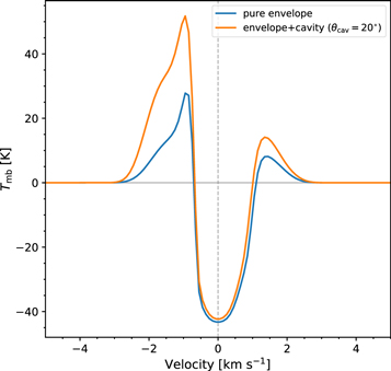
Figure 31. The synthetic continuum-subtracted 
 line profiles calculated with the envelopes with and without the outflow cavities.
Download figure:
Standard image High-resolution imageThe inclination angle is another critical parameter for the synthetic infall profile. Here, we only consider the geometric effect of the inclination angle, as the model does not include the outflowing gas. For the TSC envelope with cavities, the infall profile strongly depends on the inclination angle, which is defined in Appendix A (Figure 32). The line profiles are extracted with the size of the observed continuum source, 052 × 039 with PA = 13125. Along the LOS close to the outflow axis, the infall profile becomes narrower due to the zero abundance in the outflow cavity, which eliminates the emission at high velocity. Along the face-on view, the absorption disappears as the molecular abundance becomes zero in the cavities, and the emission from the inner edge of the envelope dominates the line profile. The inner radius of the evaporation zone is 50 au, which is 025 at 200 pc.
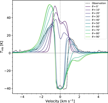
Figure 32. The synthetic continuum-subtracted infall profiles of the 
 line with inclination angles ranging from 0° to 90°. The model has a bipolar outflow with an opening angle of 20°.
Download figure:
Standard image High-resolution imageAs the inclination increases, the infall profile becomes dominated by the envelope, which consists of low-velocity warm gas and high-velocity hot gas. Thus, the intensity increases as more warm and hot gas enters the LOS, and the high-velocity emission increases from the hot gas in the evaporation zone. At high inclination, the second absorption feature appears at 2.5 km s−1 as the molecules in the evaporation zone become optically thick to the continuum source. Figure 33 shows the inclination effect in the synthetic 2D intensity maps.
Appendix C: Line-fitting Results of the ALMA Spectra
Table 9 shows the line-fitting results using class,16 a data reduction and analysis package for radio observations. The line fitting starts with a single Gaussian profile. If a single Gaussian profile fails to reproduce the spectral feature, we tried a double or triple Gaussian profile to achieve a better fit. Also, the line width is sometimes fixed to 3.5 km s−1 in order to fit blended lines. Table 9 also lists the adopted methods other than the default single Gaussian profile, and the source size fitted with 2D Gaussian profiles, using the CASA imfit task.
Table 9. Line Fitting
| Line No. | Frequency | Line Width | Integrated Flux | Deconvolved FWHMs | PA | Methoda |
|---|---|---|---|---|---|---|
| (MHz) | (km s−1) | (K km s−1) | (arcsec) | (deg.) | ||
 
|
||||||
| 1 | 354442.15 (0.07) | 3.5 (n/a) | 10.5 (0.3) | 061 ± 006 × 019 ± 004 |
16076 ± 417 |
DG/FW |
| 2 | 354445.94 (0.07) | 3.5 (n/a) | 11.3 (0.3) | 075 ± 006 × 017 ± 004 |
16393 ± 237 |
DG/FW |
| 3 | 354459.44 (0.06) | 6.6 (0.1) | 20.9 (0.3) | 048 ± 007 × 015 ± 009 |
1634 ± 868 |
|
| 4 | 354476.57 (0.08) | 7.7 (0.2) | 16.3 (0.3) | 055 ± 011 × 018 ± 013 |
16471 ± 1074 |
|
| 5 | 354525.27 (0.13) | 9.1 (0.4) | 28.4 (0.9) | 067 ± 007 × 027 ± 007 |
1621 ± 654 |
|
| 6 | 354600.95 (0.12) | 5.9 (0.2) | 15.1 (0.5) | 045 ± 011 × 022 ± 012 |
15946 ± 2335 |
|
| 7 | 354607.97 (0.02) | 3.8 (0.0) | 16.6 (0.2) | 053 ± 006 × 021 ± 006 |
16672 ± 783 |
|
| 8 | 354622.82 (0.05) | 3.3 (0.1) | 8.0 (0.2) | 055 ± 014 × 023 ± 019 |
17644 ± 1962 |
|
HCN 
|
||||||
| 9 | 356626.83 (0.03) | 3.6 (0.1) | 10.1 (0.1) | 063 ± 010 × 025 ± 006 |
15283 ± 826 |
|
| 10 | 356661.53 (0.12) | 7.5 (0.3) | 7.6 (0.2) | 062 ± 028 × 018 ± 014 |
16176 ± 4095 |
|
| 11 | 356675.94 (0.05) | 2.6 (0.1) | 2.1 (0.1) | 054 ± 027 × 017 ± 002b
|
13284 ± 398b
|
|
| 12 | 356686.39 (0.08) | 3.0 (0.2) | 2.5 (0.1) | 045 ± 019 × 025 ± 006b
|
11121 ± 1471b
|
|
| 13 | 356697.01 (0.07) | 2.3 (0.1) | 3.2 (0.1) | 050 ± 026 × 026 ± 019 |
834 ± 3752 |
|
| 14 | 356705.68 (0.05) | 2.4 (0.1) | 3.3 (0.1) | 034 ± 021 × 028 ± 019 |
17546 ± 8537 |
DG |
| 15 | 356712.81 (0.05) | 6.1 (0.1) | 14.2 (0.2) | 039 ± 013 × 029 ± 014 |
16422 ± 5856 |
DG |
| 16 | 356723.39 (0.12) | 2.9 (0.1) | 7.6 (0.1) | 058 ± 014 × 046 ± 014 |
2316 ± 6277 |
TG |
| 17 | 356726.06 (0.12) | 2.0 (0.1) | 4.4 (0.1) | 051 ± 011 × 022 ± 017 |
511 ± 1743 |
TG |
| 18 | 356729.28 (0.12) | 1.9 (0.1) | 3.2 (0.1) | 046 ± 014 × 031 ± 019 |
4273 ± 13522 |
TG |
| 19 | 356755.67 (0.07) | 6.0 (0.2) | 15.7 (0.4) | 092 ± 011 × 027 ± 008 |
1696 ± 435 |
TG |
| 20 | 356761.86 (0.14) | 3.1 (0.2) | 3.9 (0.4) | 047 ± 012 × 034 ± 015 |
3008 ± 8425 |
TG |
| 21 | 356767.25 (0.13) | 3.5 (0.3) | 4.4 (0.3) | 068 ± 025 × 028 ± 013 |
17158 ± 3066 |
TG |
| 22 | 356796.28 (0.08) | 4.9 (0.2) | 17.5 (0.6) | 066 ± 008 × 021 ± 007 |
17506 ± 586 |
|
| 23 | 356831.65 (0.04) | 1.6 (0.1) | 1.5 (0.1) | 037 ± 024 × 021 ± 007b
|
5303 ± 2259b
|
DG |
| 24 | 356834.87 (0.05) | 3.2 (0.1) | 3.9 (0.1) | 043 ± 034 × 006 ± 026 |
17054 ± 3133 |
DG |
CS 
|
||||||
| 25 | 342782.23 (0.12) | 9.4 (0.3) | 13.3 (0.3) | 039 ± 017 × 006 ± 009 |
13537 ± 2555 |
|
| 26 | 342935.06 (0.12) | 3.7 (0.4) | 10.7 (0.7) | 054 ± 011 × 020 ± 014 |
16708 ± 1399 |
|
| 27 | 342946.84 (0.08) | 4.5 (0.2) | 11.8 (0.4) | 079 ± 014 × 040 ± 010 |
17342 ± 1293 |
|
| 28 | 342997.61 (0.07) | 6.8 (0.2) | 11.3 (0.3) | 028 ± 018 × 012 ± 009 |
14282 ± 2405 |
|
H13CN 
|
||||||
| 29 | 345132.49 (0.07) | 3.5 (0.1) | 11.2 (0.4) | 052 ± 006 × 026 ± 005 |
16494 ± 102 |
|
| 30 | 345143.86 (0.11) | 3.5 (n/a) | 3.5 (0.1) | 047 ± 023 × 008 ± 011 |
14508 ± 3091 |
DG/FW |
| 31 | 345149.14 (0.09) | 3.5 (n/a) | 4.0 (0.1) | 065 ± 019 × 003 ± 013 |
15456 ± 946 |
DG/FW |
| 32 | 345162.02 (0.16) | 8.7 (0.4) | 7.7 (0.3) | 031 ± 017 × 007 ± 027 |
1609 ± 6229 |
|
| 33 | 345179.92 (0.31) | 12.1 (0.6) | 9.8 (0.4) | 038 ± 008 × 026 ± 003b
|
1600 ± 1282b
|
|
| 34 | 345209.92 (0.24) | 5.4 (0.2) | 7.5 (0.2) | 046 ± 012 × 014 ± 009 |
16695 ± 1718 |
TG |
| 35 | 345219.31 (0.24) | 4.7 (0.2) | 3.7 (0.2) | 056 ± 012 × 030 ± 004b
|
1047 ± 72b
|
TG |
| 36 | 345227.49 (0.24) | 5.1 (0.2) | 5.8 (0.2) | 051 ± 014 × 024 ± 010 |
14258 ± 2279 |
TG |
| 37 | 345235.81 (0.24) | 1.8 (0.2) | 1.9 (0.2) | 036 ± 022 × 027 ± 018 |
8992 ± 8665 |
DG |
| 38 | 345238.35 (0.24) | 1.6 (0.2) | 1.6 (0.2) | 055 ± 024 × 025 ± 018 |
12519 ± 7934 |
DG |
| 39 | 345246.53 (0.23) | 10.8 (0.7) | 9.6 (0.5) | 045 ± 019 × 037 ± 031 |
8018 ± 8475 |
|
| 40 | 345257.27 (0.17) | 5.5 (0.5) | 5.4 (0.3) | 078 ± 015 × 032 ± 003b
|
16472 ± 437b
|
|
| 41 | 345283.15 (0.08) | 4.6 (0.2) | 9.2 (0.3) | 045 ± 009 × 024 ± 008 |
15998 ± 2063 |
DG |
| 42 | 345286.34 (0.05) | 1.1 (0.1) | 1.2 (0.2) | 058 ± 009 × 033 ± 003b
|
16457 ± 685b
|
DG |
| 43 | 345295.18 (0.03) | 3.6 (0.1) | 6.7 (0.1) | 056 ± 011 × 014 ± 006 |
15786 ± 835 |
DG |
| 44 | 345300.73 (0.05) | 2.9 (0.1) | 3.2 (0.1) | 054 ± 010 × 029 ± 003b
|
15773 ± 649b
|
DG |
| 45 | 345306.00 (0.33) | 3.5 (n/a) | 3.7 (0.4) | 057 ± 021 × 024 ± 016 |
14329 ± 3365 |
FW |
| 46 | 345319.30 (0.11) | 3.5 (n/a) | 12.8 (0.5) | 052 ± 005 × 018 ± 006 |
1683 ± 629 |
DG/FW |
| 47 | 345324.74 (0.34) | 3.5 (n/a) | 4.8 (0.5) | 044 ± 006 × 030 ± 003b
|
14778 ± 986b
|
DG/FW |
| 48 | 345398.61 (0.06) | 3.6 (0.1) | 8.0 (0.2) | 048 ± 009 × 018 ± 008 |
15698 ± 1165 |
|
| 49 | 345406.47 (0.00) | 3.5 (n/a) | 4.2 (0.2) | 048 ± 007 × 034 ± 003b
|
15865 ± 1142b
|
DG/FW/FC |
| 50 | 345410.51 (0.06) | 3.5 (n/a) | 6.1 (0.2) | 039 ± 011 × 021 ± 014 |
16546 ± 2893 |
DG/FW |
| 51 | 345444.94 (0.07) | 2.1 (0.2) | 4.2 (0.5) | 051 ± 009 × 021 ± 010 |
17277 ± 1321 |
DG |
| 52 | 345448.79 (0.41) | 6.9 (0.6) | 7.3 (0.8) | 044 ± 017 × 027 ± 019 |
10881 ± 6736 |
DG |
| 53 | 345459.96 (0.13) | 5.1 (0.3) | 6.8 (0.3) | 043 ± 005 × 039 ± 005b
|
5347 ± 5424b
|
|
| 54 | 345466.71 (0.15) | 3.5 (n/a) | 6.9 (0.3) | 042 ± 010 × 025 ± 016 |
753 ± 2913 |
FW |
| 55 | 345473.52 (0.09) | 3.5 (n/a) | 4.0 (0.1) | 030 ± 013 × 022 ± 011 |
180 ± 8598 |
DG/FW |
| 56 | 345477.96 (0.13) | 3.5 (n/a) | 2.6 (0.1) | 050 ± 011 × 024 ± 002b
|
11556 ± 491b
|
DG/FW |
| 57 | 345485.49 (0.42) | 2.7 (0.7) | 4.0 (1.2) | 033 ± 010 × 011 ± 017 |
160 ± 3558 |
TG |
| 58 | 345488.34 (0.38) | 2.2 (0.8) | 2.6 (1.4) | 043 ± 015 × 021 ± 016 |
1749 ± 3347 |
TG |
| 59 | 345492.06 (0.34) | 3.0 (0.6) | 2.9 (0.6) | 051 ± 010 × 041 ± 007b
|
5249 ± 3088b
|
TG |
| 60 | 345509.46 (0.07) | 4.9 (0.1) | 10.0 (0.2) | 029 ± 009 × 015 ± 009 |
113 ± 3302 |
⋯ |
| 61 | 345546.66 (0.06) | 3.9 (0.1) | 3.8 (0.1) | 047 ± 021 × 005 ± 016 |
15985 ± 3331 |
⋯ |
| 62 | 345570.54 (0.10) | 3.3 (0.2) | 3.9 (0.2) | 048 ± 009 × 031 ± 004b
|
15065 ± 1141b
|
⋯ |
Notes. The uncertainties of each line width are shown inside the parentheses when the line width remains flexible for the fitting.
aDG: Double Gaussian; TG: Triple Gaussian; FW: Fixed line widths; FC: Fixed line centroids. bOne (or both) of the fitted FWHMs is smaller than the beam size. The fitted convolved sizes are shown instead. Such situation is typical for weak lines close to 3σ.Appendix D: Identified COMs
O-bearing molecules—Methanol (CH3OH): We identified seven emission lines of methanol and its isotopologues, including CH3OH, 13CH3OH, CH2DOH, and CH3OD. According to Anderson et al. (1988), our observations only cover one line of CH3OD, which is detected as Line 46. Parise et al. (2006a) Previous observations (Garay et al. 1998; Parise et al. 2006a) have detected the emission of methanol (CH3OH), supporting the identification of methanol. The emission of methanol (Line 9) exhibits absorption at the line center, suggesting that the emission of methanol is optically thick, so the fitted column density serves as a lower limit. If we exclude Lines 2 and 46, which are either blended with an unidentified line or had their line widths fixed during the line fitting, the mean width of methanol and its isotopologues is 3.7 ± 0.2 km s−1.

Figure 33. Intensity maps of the best-fitting  model viewed from different inclination angles. Second row shows the morphology at the blueshifted velocities from 0 km s−1 > v − vsource > −5 km s−1. Third row shows the morphology at the redshifted velocities from 5 km s−1 > v − vsource > 0 km s−1. This model is ray-traced without the central continuum source, to highlight the effects of cavities and inclinations. Inclination angles shown here follow the same definition in Section 1. An inclination of 50° shown here is equivalent to the inclination of BHR 71 (130°), but flipped upside down.
Download figure:
Standard image High-resolution imageFigure 34 shows the morphology of methanol and its isotopologues. Excluding the offset emission at the same frequency as Line 2 (see Section 7), all the emission of methanol and its isotopologues extends in the north–south direction, except for one of the CH2DOH lines (Line 13).
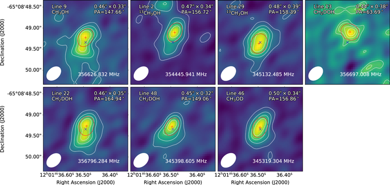
Figure 34. Moment 0 maps of methanol and its isotopologues (13CH3OH, CH2DOH, and CH3OD), calculated with a line width of 3.5 km s−1. White contours show the emission from the maximum to 3σ level. Red contour indicates the fitted size of the half power beamwidth (HPBW). Red cross shows the center of the fitted profile. Blue "×" indicates the peak of the continuum emission.
Download figure:
Standard image High-resolution imageMethyl formate (CH3OCHO): The ALMA observations detect methyl formate in both the ground state and its first torsional excited state. The ground-state rotational transitions correspond to the emission of Lines 15, 53, 54, and 57, while the emission of the vibrationally excited methyl formate matches Lines 12, 31, 39, 55, 60, and 62. The complex features of Lines 54 and 57/58 hint that the emission of methyl formate may be optically thick. A more detailed model dedicated to methyl formate may better constrain its properties.
Figure 35 shows the morphology of methyl formate in both its ground state and the vibrational excited state. One of the ground-state transitions (Line 7) peaks both north and south of the continuum source, while another ground-state transition (Line 15) peaks at the center with extended emission toward north. The rest of the methyl formate transitions (10 of 12) show a compact emission peaked at the center.
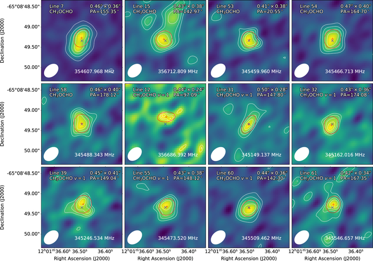
Figure 35. Similar to Figure 34, but for methyl formate (CH3OCHO).
Download figure:
Standard image High-resolution imageAcetone (CH3COCH3): Line 25 provides the strongest indication of acetone, which also matches Lines 11, 18, 40, and 45. The emission of acetone also appears at Lines 10, 23 and 24, but our simple model underestimates the strengths of these lines. Acetone emits from a compact region with a size of the continuum at the center (Figure 36).
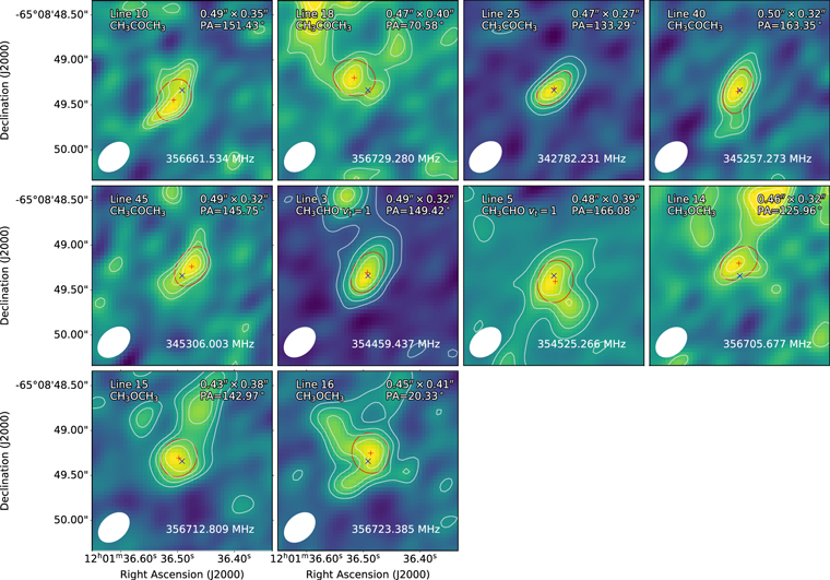
Figure 36. Similar to Figure 34, but for acetone (CH3COCH3), acetaldehyde (CH3CHO), and dimethyl ether (CH3OCH3).
Download figure:
Standard image High-resolution imageDimethyl ether (CH3OCH3): The emission of dimethyl ether matches Lines 14, 15, and 16. The apparent absorption at the center of Line 16 suggests that this transition of dimethyl ether may be optically thick. All transitions of dimethyl ether peak at the center, with an irregular morphology (Figure 36).
Ethanol (C2H5OH): The window centered on the H13CN  line detects the emission of gauche-ethanol, a conformer of ethanol, where the hydrogen of the OH group points toward hydrogens of the methyl group. The gauche form dominates in the gas phase, because of its twofold degeneracy (Scheiner & Seybold 2009). Moreover, the transitions of gauche-ethanol has lower upper energies, compared to ∼1000 K for trans-ethanol. Our model of gauche-ethanol matches Lines 33, 36, 43, 49/50, as well as the red wing of the H13CN
  line. Lines 49 and 50 heavily blend with each other, and the peak frequency of gauche-ethanol lies between the two identified peaks. The identified gauche-ethanol emission shows a compact feature peaked at the center (Figure 37).
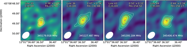
Figure 37. Similar to Figure 34, but for gauche-ethanol (gauche-C2H5OH).
Download figure:
Standard image High-resolution imageS-bearing molecules—Sulfur dioxide (SO2): Line 19 agrees with the emission of sulfur dioxide, which blends with another line, possibly CH3C15N, in its blue wing. The emission of SO2 extends over a 1'' × 1'' region, more than other identified complex molecules, peaking both north and south of the continuum source (Figure 38).
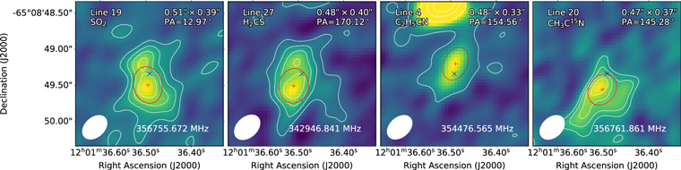
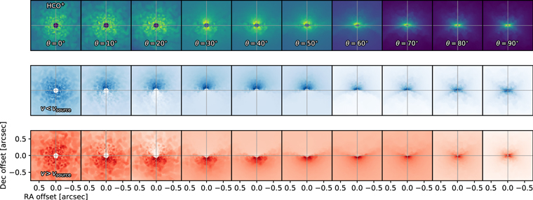
Figure 38. Similar to Figure 34, but for sulfur-bearing molecules, SO2 and H2CS, and complex cyanides, CH3C15N and C2H5CN.
Download figure:
Standard image High-resolution image
Thioformaldehyde (H2CS): The emission of thioformaldehyde agrees with Line 27. The emission of H2CS has a morphology similar to that of SO2, which is more extended than other molecules (Figure 38).
Appendix E: Tentatively Identified COMs
The species discussed here are categorized as tentatively identified because our observations do not cover enough unblended lines to support a confirmed identification. In particular, the three lines of CH3NH2 covered by our observations yield a conflicting result; thus, we only discuss CH3NH2 as a possible identification.
O-bearing molecules—Acetaldehyde (CH3CHO): The torsionally excited acetaldehyde contributes to Lines 3 and 5; however, both lines have complex line profiles due to blending with other lines. Together with the emission of HCN v2 = 1, the model of acetaldehyde reproduces the width of Line 3, but it only reproduces part of the complex profile of Line 5. Line 3 appears as a compact source centered on the continuum source, while Line 5 has more extended emission toward the south, with a peak at the center (Figure 36).
N-bearing molecules—Hydrogen cyanide (HCN v2 = 1): Together with the torsionally excited acetaldehyde, the emission of hydrogen cyanide from a vibrational excited state (v2 = 1) successfully reproduces Line 3, which is significantly broader than the other lines. While hydrogen cyanide is abundant in protostellar environments, a vibrational transition of HCN ( ) has an Einstein-A coefficient (1.3 s−1; Evans et al. 1991) much greater than that of the rotational transition of vibrationally excited HCN (A = 1.9 × 10⁻³ s−1 for
  ). Thus, the detection of the rotational emission in the vibrational excited state suggests a mechanism such as radiative pumping to keep HCN vibrationally excited.
Methyl cyanide (CH3C15N): Two lines of CH3C15N fall in the range of the observations, which are consistent with Line 20 and the blue wing of the 
 line. The extended emission of CH3C15N peaks south of the continuum source (Figure 38).
Ethyl cyanide (CH3CH2CN): The emission of ethyl cyanide contributes to Line 4 as well as the unlabelled feature at the lower-frequency end of Line 22. At Line 4, the emission of ethyl cyanide appears to be compact around the center (Figure 38).
Methylamine (CH3NH2): Three lines of methylamine fall in the range of our observations, while two of them are detected as the blue wing of Line 5 and Line 6. The line at 345,520 MHz is not detected. However, lowering the excitation temperature to ∼70 K would make the line at 345,520 MHz as weak as the noise in our observations. Thus, methylamine is the best candidate for these lines; however, it cannot be unambiguously confirmed.
Cl-bearing molecules—Methyl chloride (CH3Cl): Gauche-ethanol alone cannot fully describe the strength of the blended Line 49 and 50. Our observations cover four lines of methyl chloride, which are detected with low S/N as Lines 49/50, 52, 53, and the emission at ∼345,435 MHz. Due to the low S/N of these lines, our spectra cannot unambiguously confirm the identification of methyl chloride.