


Abstract
We present high-resolution spectroscopy of mid-infrared molecular emission from two very active T Tauri stars, AS 205 N and DR Tau. In addition to measuring high signal-to-noise line profiles of water, we report the first spectrally resolved mid-infrared line profiles of HCN emission from protoplanetary disks. The similar line profiles and temperatures of the HCN and water emission indicate that they arise in the same volume of the disk atmosphere, within 1–2 au of the star. The results support the earlier suggestion that the observed trend of increasing HCN/water emission with disk mass is a chemical fingerprint of planetesimal formation and core accretion in action. In addition to directly constraining the emitting radii of the molecules, the high-resolution spectra also help break degeneracies between temperature and column density in deriving molecular abundances from low-resolution mid-infrared spectra. As a result, they can improve our understanding of the extent to which inner disks are chemically active. Contrary to predictions from HCN excitation studies carried out for AS 205 N, the mid-infrared and near-infrared line profiles of HCN are remarkably similar. The discrepancy may indicate that HCN is not abundant beyond a few au or that infrared pumping of HCN does not dominate at these distances.
Export citation and abstract BibTeX RIS
1. Introduction
Mid-infrared (MIR) emission from water and simple organic molecules (HCN,  ) is commonly detected in spectra of classical T Tauri stars (CTTS) measured by the Spitzer Space Telescope. The high critical densities of the detected lines (>109 cm−3), the warm temperature of the emitting gas (300–1000 K), and its modest inferred emitting area argue that the emission arises from the inner few au of the disk (Carr & Najita 2011; Salyk et al. 2011b; Pontoppidan et al. 2010b), the region within the snowline. These observations complement not only near-infrared rovibrational observations of CO (4.5 μm; Banzatti & Pontoppidan 2015; Brown et al. 2013a; Salyk et al. 2011a; Bast et al. 2011; Pontoppidan et al. 2011; Najita et al. 2003), water and OH (3 μm; Salyk et al. 2008; Mandell et al. 2012; Doppmann et al. 2011; Brown et al. 2013b), and organic molecules (3 μm; Mandell et al. 2012; Gibb & Horne 2013; Doppmann et al. 2008; Gibb et al. 2007), which are generally sensitive to warmer gas at smaller disk radii, but also far-infrared and submillimeter observations that probe disks beyond the snowline (e.g., Öberg et al. 2015).
The properties of the spectrally unresolved Spitzer spectra have been used to probe the chemical state of inner disks and their planet formation status. In some analyses, the abundance ratios of the organics relative to water, as inferred from simple slab models of the emission, are enhanced compared to the molecular abundances of comets (Carr & Najita 2008, 2011), which serve as surrogate probes of the more distant giant planet region of the disk, beyond the snowline. The enhanced abundance ratios of inner disks are interpreted as evidence for an active inner disk chemistry (e.g., Carr & Najita 2008). That is, disks synthesize molecules in their warm, high-density inner regions rather than merely inheriting their organic inventory from larger disk radii or from molecular clouds (e.g., Pontoppidan et al. 2014).
The Spitzer molecular emission properties may also encode chemical evidence for the formation of icy planetesimals, a potential signature of core accretion in action. As the building blocks of planets, planetesimals are fundamental to the core accretion picture of planet formation, but they are observationally elusive: it is difficult to detect a kilometer-sized rock or even a Mars-sized protoplanet embedded in a disk! These bodies are neither self-luminous nor large enough to detect directly. They are also not massive enough to produce an observable dynamical signature, e.g., by opening a gap in the disk.
The Spitzer molecular emission properties show an interesting trend in this regard. The ratio of HCN/ emission strength increases with disk mass, a trend that has been interpreted as a possible chemical fingerprint of planetesimal formation (Najita et al. 2013). Because higher mass disks are expected to form icy planetesimals and protoplanets more readily in the giant planet region of the disk, and thereby sequester water and oxygen as ice beyond the snowline, the accreting oxygen-poor disk gas leads to a carbon-rich gaseous inner disk. Modest variations in the C/O ratio of the inner disk can in principle induce large variations in the molecular abundances of the inner disk atmosphere at a level that is consistent with the range of observed molecular emission flux ratios (Najita et al. 2011).
The above inferences assume that the MIR organics and water emission probe the same region of the disk (i.e., the same disk radii and vertical height in the disk). In reality, the spectrally and spatially unresolved Spitzer data can potentially constrain only molecular emitting areas (Carr & Najita 2011), and emission radii are unconstrained. The latter can be inferred more directly from spectrally resolved emission line profiles. Here we test the assumption from Najita et al. (2013) that the organics and water emission arise from the same region by spectrally resolving the MIR HCN and  line emission from two CTTS.
Previous high spectral resolution studies of inner disk atmospheres have spectrally resolved bright water emission in a few sources, finding that the MIR line profiles are consistent with emission from gas in Keplerian rotation over a range of radii consistent with the emitting area inferred from simple slab models (Knez et al. 2007; Pontoppidan et al. 2010b; Salyk et al. 2015; J. S. Carr et al. 2018, in preparation). The present study complements these studies of water emission and resolves the line profiles of the much fainter HCN emission.
We describe our observations in Section 2 and our results in Section 3. Section 4 discusses how the results bear on our ability to probe the chemical fingerprint of planetesimal formation (Section 4.3), to measure the abundance ratios of inner disks (Section 4.4), and our understanding of the excitation of the infrared transitions of HCN (Section 4.5). We conclude with a summary (Section 5).
2. Observations
DR Tau and AS 205 N are very active CTTS with bright molecular emission, as observed with Spitzer and ground-based spectroscopy (Salyk et al. 2008; Mandell et al. 2012; Pontoppidan et al. 2010a, 2010b; Banzatti et al. 2014; Brown et al. 2013a). AS 205 N has also been well studied at millimeter wavelengths (e.g., Andrews et al. 2009; Salyk et al. 2014).
The detection with Spitzer of MIR molecular emission from AS 205 N and DR Tau, reported initially by Salyk et al. (2008), has been studied in greater detail in subsequent analyses of Spitzer spectra (Pontoppidan et al. 2010a; Salyk et al. 2011b). The water emission from AS 205 N has been studied previously at high spectral resolution using the Very Large Telescope: in the L-band with CRIRES (R ∼ 100,000) and in the MIR with VISIR (R ∼ 20,000; Pontoppidan et al. 2010b). MIR water emission from DR Tau has been studied previously with VISIR (Banzatti et al. 2014). Mandell et al. (2012) studied the L-band water and organics emission from AS 205 N (CRIRES; R ≈ 96,000) and DR Tau (Keck/NIRSPEC; R ≈ 25,000) at lower signal-to-noise than in the present study.
We observed AS 205 N and DR Tau using the high-resolution (R ∼ 80,000) cross-dispersed mode of the Texas Echelon Cross Echelle Spectrograph (TEXES; Lacy et al. 2002) on the Gemini-North 8 m telescope (Table 1). For all observations, we used a 0 5 wide slit and nodded along the slit to remove background emission. We followed the standard TEXES procedure of observing a blackbody and blank sky roughly every 6 minutes to provide wavelength calibration, flatfielding, and approximate flux calibration. In addition, we observed asteroids as telluric standards for each object. The asteroid observations also improve the removal of the instrumental signature, as they are point sources, whereas the blackbody is an extended object.
Table 1. Observation Log
| Target | Date | λ Setting | tInt | Telluric Standard | Features Targeted |
|---|---|---|---|---|---|
| DR Tau | 2013 Nov 17 | 781 cm−1 | 41 minutes | 10 Hygiea | HCN R(23),  R(21) R(21) |
| DR Tau | 2013 Nov 19 | 805 cm−1 | 20.5 minutes | 10 Hygiea |

|
| AS 205 N | 2014 Aug 17 | 781 cm−1 | 55 minutes | 15 Eunomia, 16 Psyche | HCN R(22), R(23),  R(21) R(21) |
| AS 205 N | 2014 Aug 18 | 805 cm−1 | 17.3 minutes | 15 Eunomia |

|
| AS 205 N | 2014 Aug 18 | 781 cm−1 | 35.6 minutes | 16 Psyche | HCN R(22), R(23),  R(21) R(21) |
Download table as: ASCIITypeset image
DR Tau was observed on 2013 November 17 and 19 (UT) during the TEXES visitor-instrument campaign at Gemini. We set the central wavenumber of the instrument to roughly 781 cm−1 on the first night to detect the HCN R(23) line at 782.653 cm−1 and to roughly 805 cm−1 on the second night to detect several  lines. At these wavelengths the spectral orders are wider than the TEXES detector, so there are small gaps in the spectral coverage. Similarly, we observed AS 205 N on 2014 August 17 and 18 (UT) during the next TEXES visitor-instrument campaign at Gemini. The spectral settings were similar to but slightly different from those for DR Tau, with the HCN R(22) line included in the 781 cm−1 setting.
We reduced the data using the standard TEXES pipeline (Lacy et al. 2002). The pipeline corrects for spikes, differences nod pairs, aligns the stellar continuum along the slit in each nod difference, sums the nod differences, and extracts the spectrum after weighting by the distribution of continuum emission along the slit. In addition, the user interacts with the pipeline to set the frequency scale based on atmospheric features. The frequency scale is accurate throughout the setting to 1 km s−1.
Before dividing the stellar spectrum by that of the telluric standard, the asteroid spectra were raised to a power in order to account for differences in the air mass and precipitable water vapor at which the target and calibrator were observed. This scaling makes sense in a simple plane parallel atmosphere, where the atmospheric transmission at zenith distance z is related to the transmission at zenith,  , by
, by  . Differences in air mass and water vapor column affect the strength of telluric atmospheric lines.
The DR Tau spectrum was flux calibrated by scaling the continuum to 1.87 Jy, based on the Spitzer IRS SH spectrum. Studies of the spectral variability of DR Tau show that the flux varies by ∼20% at this wavelength (Kóspál et al. 2012; Banzatti et al. 2014). For AS 205 N, we scaled the continuum to 6.0 Jy. This value was based on the IRS SH spectrum (Section 3.2) and the observed history of the primary/secondary flux ratio at 12.5 μm (Liu et al. 1996; McCabe et al. 2006). The Spitzer IRS flux is consistent with most published values for the combined flux of the binary components, although it has been observed to be brighter by 60% (Liu et al. 1996). Additional details are provided in Section 3.2.
3. Results
Table 2 reports the detected spectral features. In the 781 cm−1 setting on AS 205 N, we detected the R22 and R23 lines of the HCN v2 band, the R21 line of the  v5 band, and the rotational water lines at 779.304 and 783.762 cm−1 (Figure 1; hereafter 779 and 784 cm−1). The 784 cm−1 water line is truncated by the edge of the order, and the 779 cm−1 line is near the edge of the order and is affected by telluric absorption. In the 805 cm−1 setting, we detected the rotational water lines at 808.083, 806.696, and 805.994 cm−1 at high signal-to-noise (hereafter 808, 807, and 806 cm−1) as well as the lower energy water lines at 803.546 and 802.990 cm−1 (Figure 2; hereafter 804 and 803 cm−1). The latter two lines have higher noise as a result of telluric absorption.

Figure 1. TEXES spectrum of AS 205 N in the 781 cm−1 setting showing the detection of HCN R22 and R23,  R21, and water emission lines in the geocentric frame. Only orders containing detected features are shown. Emission features are labeled at the source velocity. The position of telluric absorption features that cause increased noise are denoted below the spectrum (magenta labels).
Download figure:
Standard image High-resolution image
Figure 2. TEXES spectrum of AS 205 N in the 805 cm−1 setting showing the detection of bright water emission lines in the geocentric frame. The order near 807.5 cm−1, which has no detected features, illustrates the typical signal-to-noise ratio in the absence of emission and strong telluric features.
Download figure:
Standard image High-resolution imageTable 2. Detected Features
| Line | Rest Waveno | Eup | Aul | AS 205 N | DR Tau |
|---|---|---|---|---|---|
| (cm−1) | (K) | s−1 | |||
| 781 cm−1 Setting: | |||||
| HCN R22 ν2 = 1–0 | 779.727 | 2197 | 1.36 | e | in gap |
 R21 ν5 = 1–0 R21 ν5 = 1–0 |
780.753 | 1905 | 3.82 | e | x |
| HCN R23 ν2 = 1–0 | 782.653 | 2299 | 1.38 | e | e |
 R22 ν5 = 1–0 R22 ν5 = 1–0 |
783.087 | 1983 | 3.86 | in gap | on edge |
 10,8,2–9,5,5 (p) 10,8,2–9,5,5 (p) |
779.304 | 3244 | 0.16 | e | poor correction |
 17,6,12–16,3,13 (p) 17,6,12–16,3,13 (p) |
783.762 | 6073 | 9.92 | on edge | x |
| 805 cm−1 Setting: | |||||
 13,7,6–12,4,9 (o) 13,7,6–12,4,9 (o) |
802.990 | 4213 | 1.05 | e | e? poor correction |
 11,8,3–10,5,6 (o) 11,8,3–10,5,6 (o) |
803.546 | 3629 | 0.29 | e | e? poor correction |
 16,3,13–15,2,14 (p) 16,3,13–15,2,14 (p) |
805.994 | 4946 | 4.22 | e | e |
 17,4,13–16,3,14 (o) 17,4,13–16,3,14 (o) |
806.696 | 5781 | 7.67 | e | e |
 16,4,13–15,1,14 (o) 16,4,13–15,1,14 (o) |
808.038 | 4949 | 4.21 | e | e |
Note. Rest wavenumbers are from HITRAN (Rothman et al. 2013). In columns (4) and (5), "e" indicates emission, "x" indicates nondetection, and "in gap" and "on edge" indicate lines that fell either in a gap between two orders or on the edge of an order.
Download table as: ASCIITypeset image
In the 781 cm−1 setting on DR Tau, we detected the HCN R23 line but not the water lines at 779 and 784 cm−1 (Figure 3). We were unable to study the HCN R22 line, which fell in a gap between two orders. The  R21 line was not detected. This is not surprising given the far lower signal-to-noise of the HCN profile and the smaller
  /HCN flux ratio at low spectral resolution of DR Tau compared to AS 205 N. In their Spitzer IRS spectra, the
  /HCN Q-band flux ratios are ∼0.5 and ∼1 for DR Tau and AS 205 N, respectively (Salyk et al. 2011b). In the 805 cm−1 setting, we detected the water lines at 808, 807, and 806 cm−1 (Figure 4). Compared to the AS 205 N spectrum, the 803 and 804 cm−1 water lines in the DR Tau spectrum are more affected by telluric absorption because of the smaller velocity shift of DR Tau at the epoch of observation (∼17 km s−1) compared to AS 205 N (∼25 km s−1). As a result, the 803 cm−1 line is detected in the DR Tau spectrum but the 804 cm−1 line is lost in the telluric absorption.

Figure 3. TEXES spectrum of DR Tau in the 781 cm−1 setting showing the detection of the HCN R23 line in the geocentric frame. The same orders shown in Figure 1 are plotted. The HCN R22 line fell between two orders, and the  R21 line was not detected.
Download figure:
Standard image High-resolution image
Figure 4. TEXES spectrum of DR Tau in the 805 cm−1 setting showing the detection of bright water emission lines in the geocentric frame. The same orders shown in Figure 2 are plotted.
Download figure:
Standard image High-resolution image3.1. Line Profiles and Velocities
To determine the HCN and  emission line profiles, we first subtracted a local linear slope to the continuum, determined from neighboring wavelength regions located just beyond the line emission region. The profiles of the bright
  lines in the 805 cm−1 setting were used to set the velocity extent of the line emission region (±25 km s−1).
The line profiles of the water and organic emission in both the AS 205 N and DR Tau spectra are consistent with each other within the noise. As shown in Figure 5, the HCN line profile in the AS 205 N spectrum is consistent with that of the  emission and with that of the weak
  line at 779 cm−1. Because the profiles of the HCN R22 and R23 lines for AS 205 N were similar, we averaged them together to obtain a higher signal-to-noise profile; the individual lines were scaled to a common line flux and the profiles averaged. The HCN emission has an FWHM of ∼20 km s−1 and peaks at vhelio ∼−4 km s−1. The top panel of Figure 5 compares the average line profile of the HCN lines (R22 and R23) with the profile of the
  R21 line. The lower panel of Figure 5 compares the average of all three organic lines (HCN R22, HCN R23, and
  R21) with the 779 cm−1 water line. The
  779 cm−1 and HCN lines are similar in strength and detected at a similar signal-to-noise ratio.

Figure 5. Comparison of organics and water line profiles in the spectrum of AS 205 N at the 781 cm−1 setting. In the top panel, the average HCN (thick black line) and  R21 (thin blue line) profiles are compared, and in the bottom panel the average of all three organic lines (HCN R22, HCN R23,
  R21; thick black line) is compared with the 779 cm−1 water line (thin blue line). The vertical scale is the normalized flux of the average of the two HCN lines (top) and the three organic lines (bottom), with the comparison feature scaled to the same peak flux. The dotted vertical line marks the peak velocity of the strong
  lines in the 805 cm−1 setting. In the bottom panel, the telluric water line, centered at −29.5 km s−1, may contribute residual water emission.
Download figure:
Standard image High-resolution imageThe bright water lines in the 805 cm−1 setting on AS 205 N provide a better estimate of the water line profile. To define the water line profile, we examined the higher energy lines, which have good telluric correction (808, 807, and 806 cm−1), and excluded the lower energy water lines (803, 804 cm−1), which have stronger telluric absorption and less certain line profiles. Figure 6 compares the average HCN line profile with the profile of the 808 cm−1  line, which is closer in excitation to the HCN lines. The profiles of the two other water lines compare similarly. All three water lines are discussed in greater detail in J. S. Carr et al. (2018, in preparation).

Figure 6. Comparison of the average HCN line profile (thin blue line) and the line profile of the 808 cm−1 water line (thick black line) for AS 205 N. The vertical scale is the normalized flux of the water line with the HCN scaled to the same peak flux. The vertical dashed line marks the centroid velocity of the three bright  lines in the 805 cm−1 setting.
Download figure:
Standard image High-resolution imageGiven the wavelength calibration uncertainty and the limited signal-to-noise ratio of the HCN profile, the water and HCN profiles appear consistent with each other. Echoing the result found here, Mandell et al. (2012) found that the line profiles of the HCN and  emission lines observed in the L-band with CRIRES were consistent with each other, although at a much lower signal-to-noise ratio.
Similar results are found for the water and HCN emission from DR Tau. Figure 7 shows the average water line profile, obtained by scaling the three bright water lines in the 805 cm−1 setting to the same equivalent width and averaging. The resulting profile is centrally peaked, with an FWHM of 13 km s−1 and centered at vhelio of 25 km s−1. The HCN line profile overlaps the  lines in velocity and appears consistent with the
  profile given the limited signal-to-noise ratio of the detection.

Figure 7. Comparison of the HCN R23 line profile (thin blue line) and the average profile of the three bright water lines observed in the 805 cm−1 setting (thick black line) in the DR Tau spectrum. The water emission is centered at 25 km s−1 (vertical dashed line).
Download figure:
Standard image High-resolution imageThe water line emission properties we measure are in good agreement with earlier observations of water emission from DR Tau. Observations with VISIR found the same vhelio for the 806 and 805 cm−1 water lines (Banzatti et al. 2014). Our measured FWHM of the MIR water emission (13 km s−1) is consistent with that of the L-band water emission from DR Tau measured with Keck/NIRSPEC (18 km s−1; Brown et al. 2013b) given the lower spectral resolution of the NIRSPEC spectrum (12 km s−1). From the NIRSPEC spectrum, Brown et al. (2013b) inferred that the water emission extends outward in disk radius to at least 0.4 au, i.e., to a projected velocity of at least 7 km s−1 for the stellar mass (0.4 M⊙; Isella et al. 2009) and source inclination (i = 13°; see also Pontoppidan et al. 2011). At the higher resolution of the TEXES observations, we find that the MIR water emission extends to lower velocities and therefore larger disk radii (Section 4.1).
More generally, the line center velocities of the molecular emission from DR Tau and AS 205 N are consistent, within the TEXES wavelength calibration uncertainty, with that of other infrared and submillimeter molecular emission from the sources and with their stellar velocities. Further details are provided in Appendix A.
3.2. Characterizing the Emission with Simple Slab Models
To characterize the detected emission, we compared the observed emission features with simple spectral synthesis models of LTE emission from gaseous slabs of a given temperature, column density, and emitting area (e.g., Carr & Najita 2008, 2011; Salyk et al. 2011b). Although protoplanetary disks are not isothermal (vertically or radially) and may not be in vibrational LTE, isothermal slab models can provide good fits to the data. They also provide estimates of the physical conditions in the line emitting regions.
For each of the two observed targets, we first calculated synthetic spectra to match the IRS SH spectra and then generated high-resolution spectra using the same model parameters for comparison with the TEXES data. The reduction of the IRS SH data for AS 205 N (2004 August 28, AOR 5646080) and DR Tau (2008 October 8, AOR 27067136) followed the methods given in Carr & Najita (2011). The procedure and molecular linelists used in the modeling are also described in Carr & Najita (2011). While the molecular emission lines are not resolved with IRS (R = 600), the IRS spectra have the advantage of including many lines with different A-values and energy levels, which constrains the temperature and column density (e.g., Carr & Najita 2008, 2011; Salyk et al. 2011b). Thus, the IRS spectra complement the TEXES data, which include only a few lines spanning a limited range of excitation.
In the slab models, the dust continuum is assumed to be negligible in the layer of the atmosphere that produces the molecular emission, consistent with our expectations for disk atmospheres. Recent disk atmosphere models by Najita & Ádámkovics (2017), which include irradiation by UV continuum and Lyα, find that warm HCN and water are abundant in the disk atmosphere over a vertical column density of NH ∼ 1022 cm−2 in hydrogen nuclei. If we assume that the dust in the atmosphere is reduced by a factor of ∼100 compared to ISM conditions, as is inferred for T Tauri disks and attributed to grain settling (Furlan et al. 2006), the vertical optical depth of the HCN-emitting region is AV ∼ 0.05 and much lower at MIR wavelengths.
3.2.1. AS 205 N
We first fit the IRS water emission spectrum from AS 205 N using synthetic spectra generated with the LTE slab emission model. As described above, the IRS spectra have the advantage of including many water lines with different A-values and energy levels, which constrains the temperature and column density (e.g., Carr & Najita 2008, 2011). The temperature and column density were determined by χ2 fits to water features between 12 and 16 μm. The best fit to the AS 205 N IRS water spectrum (Figure 18) gives a temperature of 680 ± 80 K, a column density of  = 1.3(+0.9/ −0.5) ×1018 cm−2, and an emitting area of
  where Re = 1.90 ± 0.14 au, for a distance of 130 pc (Wilking et al. 2008; Loinard et al. 2008; Mamajek 2008). The parameters are given in Table 3. Note that in fitting the IRS spectra of water, temperature and column density are correlated (Salyk et al. 2011b) such that a higher bound on temperature corresponds to a lower bound on column density and a smaller emitting area.
Table 3. Parameters for Slab Models
| Source | Spectrum | T | R | N( ) ) |
N(HCN) | N( ) ) |
N(HCN)/N( ) ) |
|---|---|---|---|---|---|---|---|
| (K) | (au) | (cm−2) | (cm−2) | (cm−2) | |||
| AS 205 N | IRS | 680 | 1.90 | 1.3 (18) | 4.2 (15) | 1.5 (15) | 0.0033 |
| AS 205 N | TEXES | 680 | 1.90 | 1.6 (18) | 6.8 (15) | 1.0 (15) | 0.0043 |
| DR Tau | IRS | 690 | 1.33 | 9.3 (17) | 5.7 (15) | 6.8 (14) | 0.0062 |
| DR Tau | TEXES | 690 | 1.33 | 4.6 (17) | 4.4 (15) | ⋯ | 0.0097 |
Note. The same temperature and emitting area are assumed for all species. For uncertainties, see text.
Download table as: ASCIITypeset image
To model the HCN and  Q branch emission (at 14 μm and 13.7 μm respectively), we subtracted the synthetic water emission from the IRS spectrum. While LTE slab models provide a general match to the IRS water spectra, the fits are far from perfect (Carr & Najita 2011; Salyk et al. 2011b). Mismatches between the observed and model spectra are likely due to a range in temperature and column density in actual disk atmospheres, non-LTE level populations, and possibly missing transitions in the water line list or other unidentified features. Of relevance to the HCN and
  modeling, the water model appears to overcorrect for the few
  features that fall within the Q branches. The location of these
  features are marked in Figures 8 and 11. The pixels affected by these lines were ignored in the modeling.

Figure 8. Spitzer IRS spectrum of HCN and  emission from AS 205 N (black line) compared with an LTE slab model (red line). The water emission model (Figure 18; see Appendix
  column densities of N(HCN) = 4.2 × 1015 cm−2 and N(
 ) = 1.5 × 1015 cm−2 and adopts the same temperature (680 K) and emitting area as those for water. Pixels affected by water emission features at the marked locations (vertical lines) were excluded from the model fit.
Download figure:
Standard image High-resolution imageIn modeling the HCN and  emission, we assumed that they have the same emitting area and temperature as the
  emission and adjusted the column density to match the flux in the Q branches. The assumption of similar emitting areas for
  , HCN, and
  is reasonable, given the similarity of their line profiles in the TEXES data. We find that the HCN and
  emission can be matched with column densities NHCN = 4.2 (±0.2) × 1015 cm−2 and
  . The shape of the Q branches is diagnostic of the rovibrational temperature of the gas. Comparison of the observed and model HCN spectra (Figure 8) shows that HCN is consistent with having the same ∼680 K temperature as
  . To explore the range of possible temperatures for the HCN emission, we held the emitting radius constant but allowed both temperature and column density to vary. This gave a best fit at T = 670 K with a range of 590–770 K, similar to the temperature range for
  . For
. For  , the smaller width of the band and the water line at 13.69 μm prevented a definite determination of its temperature.
The parameters derived from the IRS spectra (Table 3) were then used to calculate LTE model spectra for comparison to the TEXES data. The IRS parameters work well for the TEXES  spectrum: the line ratios of the three best-measured water lines are reproduced, and the line fluxes are within 15% of the observed values. For the model plotted in Figure 9, the
  column density was increased to
  = 1.6(±0.1) × 1018 cm−2 to match the line fluxes, although a small change in radius, temperature, or flux calibration would work equally well. The optical depths for the TEXES
  lines are of order unity; therefore, the ratios of the three lines depend on both water temperature and column density. The match of the IRS-based model to the TEXES data (Figure 9) shows that the TEXES and IRS water emission are consistent with the same LTE temperature, column density, and emitting area.

Figure 9. The three cleanest water emission lines in the (continuum subtracted) TEXES spectrum of AS 205 N (black line), shown in the rest frame of the emission, compared with the LTE emission model (dashed blue line) used to fit the water emission in the Spitzer IRS spectrum (Figure 18) and with a model with N( ) increased to 1.6 × 1018 cm−2 to match the observed line fluxes (red line). The model line emission has been broadened by a Gaussian profile with an FWHM of 23 km s−1.
Download figure:
Standard image High-resolution imageWhen the parameters used to fit the IRS spectra of HCN and  are applied to the TEXES spectrum (Figure 10; dotted red line) we find that the HCN lines are underpredicted by 36% while the
  line is overpredicted by 44%. A change in the joint emitting area of the molecules could not produce this effect. The line strengths in the TEXES spectrum can be fit (solid red line in Figure 10) by increasing the column density of HCN to 6.8(±0.5) × 1015 cm−2 and decreasing the column density of
  to 1.0(±0.1) × 1015 cm−2.

Figure 10. The HCN and  lines observed in the continuum-subtracted TEXES spectrum of AS 205 N, shown in the rest frame of the emission, compared with the LTE emission model (dashed blue line) used to fit the HCN and
  bands in the IRS spectrum (Figure 8). The solid red line shows a model with column densities adjusted to fit the TEXES line fluxes, in which N(HCN) = 6.8 × 1015 cm−2 and N(
 ) = 1.0 × 1015 cm−2.
Download figure:
Standard image High-resolution image3.2.2. DR Tau
The same procedure was followed for DR Tau. The fit to the IRS water spectrum of DR Tau gave T = 690 ± 75 K,  = 9.3(+6.7/−3.4) × 1017 cm−2, and Re = 1.33 ± 0.07 au, assuming a distance of 140 pc (Figure 19 in Appendix
  spectrum, the HCN and
  Q branch fluxes were fit by adjusting the column densities, assuming the same emitting area and temperature as for the
  emission. Figure 11 shows the resulting fit, with column densities of NHCN = 5.7(±0.3) × 1015 cm−2 and
  = 6.8(±1.0) × 1014 cm−2. While the
  temperature of 690 K is consistent with the shape of the HCN Q branch, a higher temperature (∼800 K) improves the fit slightly, with an acceptable range of 700–1000 K. The
  Q branch is relatively weak in DR Tau, and no conclusion about the
  temperature is possible.

Figure 11. Spitzer IRS spectrum of HCN and  emission from DR Tau (black line) compared with an LTE slab model (red line). The water model (Figure 19; see Appendix
  column densities of N(HCN) =5.7 × 1015 cm−2 and N(
 ) = 6.8 × 1014 cm−2 and adopts the same temperature and emitting area as for the water emission. Pixels affected by water emission features at the marked locations (vertical lines) were excluded from the model fit.
Download figure:
Standard image High-resolution imageWhen the water emission parameters derived from the IRS spectra are used to model the TEXES spectrum, the water line fluxes are overpredicted by nearly a factor of two (Figure 12). A reduction of the column density to  = 4.6(±0.2) ×1017 cm−2 matches the line fluxes. The temperature could also be lowered to reduce the line fluxes, but then the observed line ratios would no longer match. The model
  fluxes can also be reduced by decreasing the emitting area, or increasing the continuum flux (i.e., the flux calibration), but this would cause the HCN flux to be underpredicted. With the nominal IRS-derived model, the HCN line is overpredicted by ∼30%. To reproduce the observed HCN line strength (Figure 13) requires decreasing the HCN column density to 4.4(±0.8) × 1015 cm−2. The prediction for the
  R21 line (not shown) is consistent with the nondetecton of this line in the TEXES data.

Figure 12. The three cleanest water emission lines in the continuum-subtracted TEXES spectrum of DR Tau (black line), shown in the rest frame of the emission. The LTE model used to fit the  emission in the Spitzer IRS spectrum of DR Tau (Figure 19) overpredicts the TEXES water emission (dashed blue line). Lowering the
  column density to 4.6 × 1017 cm−2 produces a good fit (red line). In the model spectra, the emission lines were broadened by a Gaussian profile with an FWHM of 15 km s−1.
Download figure:
Standard image High-resolution image
Figure 13. The HCN R(23) line observed in the continuum-subtracted TEXES spectrum of DR Tau (black line), shown in the rest frame of the emission, compared with the LTE model (dashed blue line) used to fit the HCN band in the Spitzer IRS spectrum (Figure 11) and to a model (solid red line) with the HCN column density decreased to N(HCN) = 4.4 × 1015 cm−2 in order to fit the line flux.
Download figure:
Standard image High-resolution image3.2.3. Variability
As described above, we find changes in the derived water and HCN column densities between the IRS and TEXES observations for both AS 205 N and DR Tau (see Table 3). Because the TEXES observations were flux calibrated by adopting the continuum flux from the IRS spectra, any variation in the continum level would produce apparent changes in the line flux and the derived column density. However, a simple flux calibration scaling alone cannot explain all the observed changes because some of the discrepancies between the model and observed line fluxes differ in magnitude and sometimes in direction. Nevertheless, it is possible to compare the ratios of column densities. If the continuum spectral shape of the source is constant over the small range of TEXES wavelengths studied, the equivalent widths of the HCN and water lines will accurately reflect their relative fluxes.
Based on the above LTE slab modeling of the IRS spectra, the HCN/ column density ratio is 0.0033 (+0.0021/−0.0013) for AS 205 N and 0.0062 (+0.0033/−0.0023) for DR Tau. These uncertainties come from the range in the ratio obtained at the extremes of the confidence boundary in temperature and column density parameter space for the fit to the IRS water spectrum and are dominated by the allowed range in the water column density.
To compare the HCN/ column density ratios from the IRS and TEXES data, we calculate the uncertainty in the IRS ratio using the error in the IRS water column at a fixed temperature. This choice is consistent with our use of the temperature and Re from the IRS water spectrum in fitting the other data (Table 3) and corresponds to a ∼20% error in N(
 ) for both AS 205 N and DR Tau. The other uncertainties that matter are the measurement uncertainties in the IRS HCN band flux and the TEXES line fluxes.
Including these uncertainties in comparing the HCN/ ratios, we obtain for AS 205 N a column density ratio of HCN/
 = 0.0033 ± 0.0007 from the IRS data and 0.0043 ± 0.0004 from the TEXES data. For DR Tau, the ratios are 0.0062 ± 0.0013 from the IRS data and 0.0097 ±0.0018 from the TEXES data. While the change in the HCN/
 ratio is 30% for AS 205 N and 56% for DR Tau, the significance in the difference is modest, 1.3σ and 1.6σ respectively, providing marginal evidence for variation in the column density ratio.
One of the limitations in this comparison is the presumption that the temperature and emitting area are the same for both molecules at both epochs of observation. We found that the IRS spectra are consistent with the same temperature for  and HCN, within the uncertainties. Furthermore, the water line ratios in the TEXES spectra are consistent with the IRS-derived temperature for
  . However, there is no independent constraint on the HCN temperature for the TEXES observation. The presumption of the same emitting area is based on the similarities of the
  and HCN velocity profiles, but we can only assume that the emitting areas were the same at the time of the IRS observations.
Another limitation is that we are comparing models for low-resolution (IRS) observations of the HCN Q branch, which is a blend of rovibrational lines dominated by the v2 = 1–0 and 2–1 bands, with observations of individual lines (TEXES) in the v2 = 1–0 R branch. The upper energy level of the R-branch lines observed with TEXES is close to the flux-weighted average of lines within the observed Q branch. However, if non-LTE effects were to produce different rotational and vibrational excitation temperatures, then a temperature that fits the entire Q branch may not be the appropriate excitation temperature for the observed v2 = 1–0 lines.
All of the above assumptions can eventually be tested with multiple epochs of high-resolution spectroscopy of water and HCN that cover more transitions. By measuring a broader range in HCN line excitation, and with sufficient S/N to measure v2 = 2–1 transitions, the HCN rotational and vibrational temperatures can be determined.
4. Discussion
4.1. Emission from the Inner Disk
We find that the line profiles of the MIR HCN and  emission from DR Tau and AS 205 N are roughly symmetric and centered within a few km s−1 of the stellar velocity (Appendix A). The emission also overlaps in velocity other known molecular emission diagnostics from the inner disk regions of these sources (rovibrational CO,
  , UV fluorescent
  ; e.g., Salyk et al. 2008, 2011a; Schindhelm et al. 2012; Banzatti et al. 2014; Brown et al. 2013a, 2013b). These properties are consistent with emission from a rotating disk and not with high velocity outflows or inflows. Magnetocentrifugal winds and magnetospheric infall produce strongly blue- or redshifted emission and/or absorption features extending to ∼100 km s−1 or more even at the relatively low inclination of our sources, e.g., forbidden optical line emission from winds (Hartigan et al. 1995; Simon et al. 2016) and magnetospheric infall emission/absorption profiles observed in H i (e.g., Edwards et al. 1994; Muzerolle et al. 1998a, 1998b; Folha & Emerson 2001).
Millimeter imaging and infrared spectroastrometric studies point to a low inclination for AS 205 N (i = 15° to include the units of degrees; as discussed in Salyk et al. 2014). Inclination estimates range from low to high for DR Tau, with spectroastrometric studies of the inner disk favoring a low inclination. The Pontoppidan et al. (2011) study of CO rovibrational emission found a good fit to their data assuming an inclination of 9°. Brown et al. (2013b) were able to fit their spectroastrometric L-band water observations with an inclination of i = 13°.
Photoevaporative disk winds are expected to produce observable blueshifts of 5–10 km s−1 at these low inclinations (Font et al. 2004; Alexander 2008). In contrast, the water profiles of both sources studied here show, if anything, small redshifts rather than blueshifts. The water profile of DR Tau is +3 km s−1 from the average of the reported stellar velocities (Petrov et al. 2011; Nguyen et al. 2012), and the AS 205 N profile is shifted by +4 km s−1 (Melo 2003; Appendix A). The absence of a photoevaporative signature in the HCN and  profiles is not surprising. Driven from the disk surface by X-ray and UV irradiation, photoevaporative flows are likely to be atomic or ionized rather than molecular and unlikely to contribute to the molecular emission profile. Thus the line profiles of the HCN and
  emission are best explained as arising in the inner disk.
The resolved line profiles also constrain the range of disk radii from which the emission arises. Au-sized projected emitting areas have been inferred for the MIR molecular emission from CTTS based on Spitzer spectra, which are spatially and spectrally unresolved (Carr & Najita 2008, 2011; Salyk et al. 2011b). From simple slab emission models, we infer water-emitting areas  with an Re of 1.3 au for DR Tau and 1.9 au for AS 205 N (Section 3.2), similar to values previously reported in the literature. Salyk et al. (2011b) previously inferred water-emitting areas
  with an Re of 1.1 au for DR Tau and 2.1 au for AS 205 N using a similar approach.
Using the resolved line profiles, we can obtain an independent constraint on the range of disk radii responsible for the emission given the disk inclination and stellar mass for each source. For AS 205 N, with a stellar mass of M* = 1.1 M⊙ (Najita et al. 2015) and an inclination of i = 15, the observed ∼30 km s−1 HWZI (half-width at zero intensity) of the  emission corresponds to an inner emission radius of 0.07 au. Emission from gas at 1.7 au would have a projected velocity of v sin i = 6.2 km s−1, similar to the half-width of the flat-topped portion of the water line profile (Figure 6). Thus the line profile is consistent with
  emission extending from 0.07 au to ∼2 au. The HCN profile of AS 205 N is similar to the
  profile at low velocities, indicating that the HCN emission extends over a similar range of radii. Because of their lower signal-to-noise ratio, it is not possible to determine whether the wings of the HCN profile have the same velocity extent as the
  profile. The HCN emission extends to at least ±15 km s−1 from line center, i.e., inward in radius to at least 0.3 au.
For DR Tau, with a stellar mass of M* = 1.2 M⊙ (Andrews et al. 2013, using stellar evolutionary tracks from Siess et al. 2000) and i = 8°, the observed HWZI of at least 20 km s−1 for the  lines corresponds to an inner emission radius of 0.05 au or smaller. Emission from gas at 1.4 au would have a projected velocity of v sin i = 4 km s−1. We observe
  emission throughout this range of velocities, and the strongly peaked profile suggests that the emission may extend beyond 1.4 au. Here we have adopted a lower inclination (i = 8°) than the values preferred by Pontoppidan et al. (2011; i = 9°, M* = 1.0 M⊙) and Brown et al. (2013; i = 13°; M* = 0.4 M⊙) to compensate for the larger stellar mass adopted here.
4.2. HCN and Water Probe the Same Disk Volume
The similar line profiles and emission temperatures for HCN and water suggest that the two diagnostics probe the same volume of the disk atmosphere. First, the HCN and  profiles extend over approximately the same range of velocities in the case of both AS 205 N and DR Tau, consistent with the HCN and water emission arising from approximately the same range of disk radii in both systems. Second, the similar emission temperatures for HCN and water are consistent with the HCN and water emission arising from the same vertical height in the disk. Models of inner disk atmospheres irradiated by stellar UV and X-rays find that the gas temperature exceeds the dust temperature in the atmosphere and transitions from a hot (∼4000 K) atomic region at the top of the atmosphere to a warm molecular region (∼300–1000 K) at intermediate heights before reaching the dust temperature deeper in the atmosphere (Ádámkovics et al. 2014; Najita et al. 2011; Najita & Ádámkovics 2017). Both HCN and water are abundant in the intermediate layer—the warm molecular region—consistent with the similar line profiles and temperatures found here for the HCN and water emission.
The inferred temperatures and column densities of the HCN and water emission are also roughly consistent with thermal-chemical models of irradiated disk atmospheres. In comparison with the ∼700 K temperature and Re ∼ 1.5 au emitting area found for the HCN and  emission, the reference model of Najita & Ádámkovics (2017) for a generic T Tauri disk atmosphere irradiated by stellar far-UV continuum, Lyα, and X-rays, is characterized at 1 au by vertically coincident warm (300–1000 K) HCN and water with vertical column densities (3 × 1015 cm−2 and 2 × 1017 cm−2, respectively) similar to the measured line of sight columns (∼5 × 1015 cm−2 and ∼1 × 1018 cm−2, respectively). Closer agreement may be possible with disk atmospheres more closely matched to the star+disk properties of the sources studied here.
4.3. Chemical Fingerprint of Planetesimal Formation
Our results support the interpretation of the observed trend of increasing HCN/ emission with disk mass as a possible chemical fingerprint of planetesimal formation and core accretion in action (Najita et al. 2013; Carr & Najita 2011). The core accretion model of planet formation is compelling in its ability to account for planet formation outcomes such as the existence of small rocky planets as well as ice and gas giants within the solar system and in the exoplanet population. But what does core accretion look like? Can any observations reveal whether known protoplanetary disks are actually engaged in core accretion? One approach is to look for observational evidence of the formation of planetesimals and protoplanets, which play no role in a competing theory of planet formation such as gravitational instability.
Observationally elusive, planetesimals are difficult to detect directly because of their small size, small mass, and intrinsic faintness. However, they may potentially reveal themselves through the chemical signature they induce in the gaseous disk within the snowline. When icy objects grow large enough (kilometer-sized or larger) to decouple from inward migration induced by gas drag, they are sequestered in the icy region of the disk beyond the snow line (beyond ∼1 au; Ciesla & Cuzzi 2006). The gas that accretes into the warm inner disk region within the snow line is thereby depleted of water (and oxygen), resulting in a higher C/O ratio than the disk overall. Thermal-chemical models of disk atmospheres predict that only a modest enhancement in the C/O ratio of the inner disk (factor of 2) is sufficient to induce a large, observable change in the HCN/ ratio in the atmosphere (factor of 10), consistent with the range of observed molecular emission flux ratios (Najita et al. 2011).
As a result, molecular abundances in the inner disk (within the snow line) may encode evidence for icy planetesimal formation beyond the snowline. Because disks with higher masses are expected to grow planetesimals more rapidly, we expect to see the HCN/ ratio in the inner disk increase with disk mass in systems undergoing planetesimal formation, a trend that is indeed observed (Najita et al. 2013; see also Figure 14). If this interpretation of the observed trend is correct, it implies that most T Tauri disks are in an advanced stage of planet formation, having built and sequestered large icy bodies beyond the snow line (Najita et al. 2013). This interpretation assumes that the HCN and
  emission arise from the same volume of the disk atmosphere. In finding that MIR HCN and water emission probe the same volume of the disk atmosphere, our results support the hypothesis that the trend between the HCN/
 flux ratio and disk mass is evidence for planetesimal formation.

Figure 14. HCN/ flux ratio of inner disks vs. disk mass from fits to low-resolution Spitzer IRS spectra (red diamonds; Najita et al. 2013) and the results obtained here for AS 205 N and DR Tau from their IRS (blue diamonds) and TEXES (blue circles) spectra. The latter assume that the change in the column density ratio between the two epochs reflects time variability in the flux ratio (see text for details).
Download figure:
Standard image High-resolution imageThe inference that planet formation is well advanced in most T Tauri disks is supported by a comparison of the mass of small solids present in T Tauri disks (the dust disk mass distribution) with the solids locked up in known exoplanet populations (Najita & Kenyon 2014). The comparison shows that there are fewer small solids in T Tauri disks than in the known exoplanets. If T Tauri disks are the birthplaces of planets, their low inventory of solids implies that they are by no means unevolved "primordial disks." More likely, most of the solids in most T Tauri disks have already grown into large sizes that are invisible to millimeter observations (beyond cm sizes) and/or they have been concentrated at small radii (within a few au) where they are optically thick at millimeter wavelengths. The trend of HCN/ versus disk mass goes a step further and implies that the solids beyond the snow line have grown much beyond cm size and large enough to decouple from gas drag (i.e., kilometer-sized or larger).
This picture is consistent with the short timescale inferred for planetesimal formation in the solar system. Radiometric analyses of meteorites find that differentiated planetesimals accumulated soon after the formation of calcium aluminum inclusions (CAIs), i.e., that planetesimal formation was well underway at the onset of the T Tauri epoch of solar system history (Kleine et al. 2009; Dauphas & Chaussidon 2011).
Figure 14 plots as a function of disk mass the HCN/ flux ratio measured from IRS spectra for the sources reported in Najita et al. (2013; red diamonds) and the sources studied here (blue diamonds). The HCN flux shown includes a correction for water emission blended with the HCN Q branch. The water flux shown is the sum of the water emission features at 17.12, 17.22, and 17.36 μm, and disk masses are derived from submillimeter continuum emission (Najita et al. 2013, 2015).
The trend of HCN/ versus disk mass, while clearly apparent, has significant scatter. Multiple factors may be responsible for the scatter. The extent of planetesimal formation in the giant planet region may differ between sources of similar outer disk mass. Excitation effects may reduce HCN emission in inner disks with lower densities (Section 4.5). HCN and
  may not always probe the same volume.
Any time variability in the HCN/ emission ratio (Section 3.2.3) will also contribute to the observed scatter. Figure 14 shows the larger HCN/
 ratios we would infer from the TEXES data (blue circles) if the larger HCN/
 column density ratios found for the TEXES data (compared to the IRS data) reflect time variability (Section 3.2.3) and if the change in the inferred column density ratio (Table 3) translates into a change in the HCN/
 flux ratio. Accordingly, the flux ratios of AS 205 N and DR Tau in the TEXES data are shown enhanced by factors of 1.3 and 1.6, respectively, over their IRS flux values. The magnitude of the variability in the HCN/
 flux ratio found for AS 205 N and DR Tau is similar to the magnitude of the scatter observed in the relationship of HCN/
 versus disk mass. (The overall trend of HCN/
 flux ratio with disk mass extends, of course, over a much larger range of values.) Further study of variability in HCN/
 ratio is needed to understand whether this range of variability is typical of T Tauri disks.
Changes in molecular emission from the inner disk could arise from changes in the instantaneous UV field (driven by variations in stellar accretion), instantaneous local accretion heating (e.g., from time-varying energy dissipation due to the magnetorotational instability), grain settling or dust-lofting events in the disk atmosphere (e.g., due to disk turbulence), or other effects. These processes affect the photochemistry of the disk atmosphere, the depth of the warm disk atmosphere that can produce MIR molecular emission, and the depth to which we can see into the atmosphere. Because the HCN emission tends to be concentrated toward the top of the atmosphere, whereas water emission can extend deeper (e.g., Najita & Ádámkovics 2017), these processes can enhance or reduce the HCN/ flux ratio.
A concrete illustration of the role of one process, accretion heating, in altering the molecular emission ratio comes from observations of the extreme outburst observed from EX Lupi (Banzatti et al. 2012). The Spitzer water emission increased dramatically in outburst, while emission from the organics completely disappeared. More modest accretion variability may produce more modest changes in the relative molecular fluxes.
4.4. Inner Disk Molecular Abundances
Our constraints on the range of disk emission radii for HCN and water also bear on the abundance ratios inferred for inner disks. Molecular abundances can probe the extent to which inner disks are chemically active, i.e., whether inner disks actively synthesize molecules or primarily inherit their abundances from the interstellar medium or larger disk radii. As noted in Section 1, some earlier analyses of spectrally unresolved data inferred that inner disks have an HCN/water abundance that is significantly enhanced, by about an order of magnitude, relative to that of comets (Carr & Najita 2008, 2011). If comets are a surrogate probe of the chemical conditions in the giant planet region of the disk, where they are believed to have formed, the difference between the abundances of inner disks and comets can be interpreted as evidence for an active inner disk chemistry.
The low spectral resolution of Spitzer/IRS introduces potential uncertainty in the inferred column density ratios and abundances, because lines are blended and the spatial information from resolved line profiles is unavailable. In general, there can be signficant degeneracies between model parameters, even for LTE slab models (Carr & Najita 2011; Salyk et al. 2011b). Modeling assumptions may also differ.
In their modeling of Spitzer IRS spectra, Carr & Najita (2008, 2011) favored a fit with a smaller emitting area for HCN than water. In their minimum chi-square fits, in which the HCN emission is close to optically thick, the HCN emitting area is a factor of 3–12 smaller than the water emitting area, and the HCN/ column density ratio is high (0.03–0.1; Figure 15, open red squares). In contrast, under the assumption of equal emitting areas for HCN and water, the HCN emission is optically thin, and the HCN/
 column density ratios are 4–30 times smaller than in the best fit but still fall within the confidence interval of fits to the HCN bandhead (see Carr & Najita 2011; Figure 15, solid red squares).

Figure 15. Column density ratios of HCN and  relative to water for LTE slab fits to Spitzer IRS and TEXES spectra compared to cometary abundances. Model fits to IRS spectra that have equal emitting areas for HCN,
  , and water (red squares—Carr & Najita 2011; magenta symbols—Salyk et al. 2011b) are closer to the abundances of comets (blue symbols; Dello Russo et al. 2016) than models that allow for different emitting areas of HCN and water (open red squares; Carr & Najita 2011). The TEXES spectra indicate similar emitting areas for the HCN and water emission from AS 205 N and DR Tau (large red circles with black dots) and fall close to the fits to their IRS spectra assuming equal emitting areas (red diamonds). Several sources from Salyk et al. (2011b) fall outside the boundaries of the plot. The range of abundances measured for hot cores are also shown (green cross; see Carr & Najita 2011 for details). The dashed lines indicate constant ratios of
  /HCN = 0.1 and 1 (short-dashed and long-dashed lines, respectively). Blue inverted triangles indicate upper limits.
Download figure:
Standard image High-resolution imageSalyk et al. (2011b) also reported molecular column densities from simple slab fits to Spitzer IRS spectra under the assumption of equal emitting areas for all molecules. In contrast to the smaller wavelength region studied by Carr & Najita (2011; 12–16 μm), Salyk et al. (2011b) fit the strengths of water emission features from a much broader range of wavelengths (10–35 μm), among other differences in the modeling procedure. As shown in Figure 15, the molecular column density ratios reported by Salyk et al. (magenta squares) do not overlap those of Carr & Najita (2011; solid red squares), illustrating how different modeling choices (e.g., wavelength region studied, assumed line broadening, weight given to individual spectral features) can lead to different results, even in the context of simple slab models. In general, Salyk et al. found lower emission temperatures and higher column densities for water, a result that pulls the molecular column density ratios in Figure 15 toward the lower left of the plot.
Now with velocity-resolved spectra of water and HCN in hand—data that directly constrain molecular emitting radii and resolve line blends—we have, for the first time, an opportunity to directly assess some of the degeneracies in modeling Spitzer IRS spectra. For the two sources studied here, we find that the high-resolution water spectra are consistent with the high-temperature, low-column-density interpretation of the Spitzer water emission (see also J. S. Carr et al. 2018, in preparation). Similarly, we find that AS 205 N and DR Tau have approximately equal HCN and water emitting areas, which helps distinguish between high- and low-column-density solutions for the HCN emission as well. Assuming that the Spitzer HCN emission temperature applies to the TEXES HCN emission, the Spitzer and TEXES spectra can be fit with similar HCN/ column density ratios.
The Spitzer HCN/ column density ratios (Figure 15, red diamonds) are 0.0033 for AS 205 N and 0.0062 for DR Tau; the TEXES HCN/
 column density ratios (Figure 15, large red circles with black dots) are 0.0043 for AS 205 N and 0.0097 for DR Tau (3.2; Table 3). These values agree with the low end of the HCN/
 column density ratios reported by Carr & Najita (2011) and are closer to the average value of comets (blue symbols). For comparison, the range of molecular abundances measured for hot cores is also shown in Figure 15 (green cross).
These results endorse some aspects of earlier work and also suggest the need to extend our study to a wider variety of sources. We confirm for the two sources studied here that simple slab fits to their IRS spectra (following the methodology of Carr & Najita 2011) are consistent with the properties inferred from their TEXES spectra (Section 3.2). These results suggest a measure of confidence in our ability to infer abundances from lower resolution data. If the equal HCN and water emitting areas we find for the sources studied here also apply to the sources studied by Carr & Najita (2011), their HCN/ column density ratios will be lower than the favored best-fit values and thereby alter our view of the level of chemical activity in inner disks. However, the results obtained here may not apply to other CTTS because AS 205 N and DR Tau are both very active sources with high accretion rates. High spectral resolution observations, similar to those presented here but of more typical T Tauri stars (like those studied in Carr & Najita 2011), are likely critical in order to measure with confidence molecular column density ratios that can be usefully compared to the abundances of comets and hot cores.
4.5. Excitation of HCN
Finally, our results bear on models for the excitation of HCN. Bruderer et al. (2015) studied the possibility of non-LTE excitation of HCN, including excitation by collisions with  and radiative pumping by infrared photons. They concluded that infrared pumping is the major excitation mechanism for rovibrational HCN emission. This was particularly true for the 3 μm lines of the v1 band, because the high critical densities of these transitions (
 ) are only present in their disk model well below the dust photosphere of the inner disk; the excitation of these transitions above the disk photosphere therefore relies on radiative pumping. In contrast, the critical density of the 14 μm lines of the v2 band is lower (∼1011 cm−3), and collisional excitation could affect the 14 μm emission from the inner 2 au of their disk model.
Using a disk model calculated specifically for the case of AS 205 N, Bruderer et al. predicted 3 and 14 μm line profiles and intensities for the HCN emission from the disk. They found that the 3 and 14 μm lines can have substantially different line profiles and that infrared pumping can excite the transitions in both bands out to large radii (∼10 au), producing very narrow line profiles.
To test these predictions, we compared the HCN line profiles of AS 205 N measured with TEXES in the MIR with the 3 μm line profiles from CRIRES (Mandell et al. 2012). We obtained an average profile for the 3 μm lines by averaging together the P5, P11, P12, and P13 lines, the cleanest HCN lines in the spectrum. The average 3 μm profile is compared to our average profile for the MIR lines in Figure 16. The MIR and 3 μm HCN profiles are remarkably similar.

Figure 16. Comparison of the velocity profiles of the MIR and 3 μm HCN emission lines in AS 205 N observed with TEXES and CRIRES, respectively. The MIR profile (black) is the average of the R(22) and R(23) transitions of the ν2 vibrational band. The 3 μm profile (red) is the average of the P(5), P(11), P(12) and P(13) transitions of the ν1 band. The profiles have been shifted to center on zero velocity. The similarity of the line profiles differs dramatically from the non-LTE predictions of Bruderer et al. (2015).
Download figure:
Standard image High-resolution imageThe velocity width for both line profiles (FWHM ∼ 20 km s−1) is much larger than the ∼10 km s−1 predicted by the Bruderer et al. models in which HCN is excited by infrared pumping out to ∼10 au. The discrepancy implies that either HCN is not abundant beyond a couple of au or that infrared pumping does not dominate at these radii. The Bruderer et al. model that best fits our observed width for the MIR lines is the "jump" model (see their Figure 10) in which the HCN abundance is assumed to be greatly reduced beyond ∼2 au. The radius of the abundance decrement is consistent with the emitting area derived from our modeling of the IRS spectra (Section 3.2). However, the same jump model also predicts a 3 μm line that is enhanced by radiative pumping and is much broader (∼45 km s−1) than observed.
Collisional excitation is most likely the dominant excitation mechanism for the 14 μm HCN band. From fitting the Q branch at 14 μm (Section 3.2.1), we know that higher vibrational states, up to at least v2 = 3, must be populated. Populating these vibrational states via infrared pumping would be difficult because of their weak radiative connection to the ground state. In the Bruderer et al. models, collisional excitation was found to be important for the 14 μm lines in the inner 2 au of the disk, consistent with our observed line profiles. The critical density of the HCN lines we observed with TEXES is ∼1011 cm−3, not much higher than those of the observed rotational water lines  ) and similar to the density in disk atmosphere models where HCN is abundant (Ádámkovics et al. 2014; Najita & Ádámkovics 2017). All of this argues that the 14 μm transitions could be close to LTE.
The role of radiative pumping in exciting the 3 μm and MIR HCN lines is unclear, as the specific line profiles predicted by Bruderer et al. are not confirmed by the observations. The 3 μm profile is indistinguishable from the MIR profile, showing that they form over the same range of radii and suggesting that the two bands could share the same excitation mechanism. If radiative pumping does play a role, the details of how the radiative excitation occurs must differ from the description put forth in Bruderer et al. (2015).
In addition to comparing the line profiles, we can also compare the expected LTE emission line fluxes with the observed fluxes. Using the LTE slab model that we used to fit the Q branch of the 14 μm band in the IRS spectrum, we predicted the strength of the 3 μm HCN lines and compared it with the 3 μm line strength from Mandell et al. (2012; Figure 17). The simple LTE model produces a good match to the 3 μm HCN line flux in the CRIRES spectrum, better than the same model applied to the TEXES data (Figure 12). One should note that neither the CRIRES spectrum nor the TEXES spectrum were independently flux calibrated, and both these and the Spitzer IRS spectrum were observed years apart. Nevertheless, the intensity of the 3 μm and MIR lines, as studied here, are consistent with HCN being close to LTE.

Figure 17. The CRIRES spectrum of HCN emission at 3 μm (black line) compared with an LTE model for the emission (red line) in the rest frame of the emission. The three plotted emission lines are the P(11), P(12), and P(13) transitions of the 1000–0000 band. The model is the same LTE model that fits the 14 μm Q branch in Figure 8.
Download figure:
Standard image High-resolution imageThe similar 3 μm and MIR line profiles for AS 205 N, the warm vibrational temperature (≳700 K) implied by the fit to the 14 μm band in the IRS spectra, and the flux ratio of the 3 μm and MIR lines are all consistent with collisional exciation of the HCN within 1–2 au of the star. However, a significant uncertainty is whether the high densities required for collisional excitation of the 3 μm lines ( see Bruderer et al. 2015, Figure 4) are present in the region of the disk atmosphere where the HCN emission forms or whether a different excitation path is required to understand the observed 3 μm HCN transitions.
One possibility is that HCN is excited by collisions with atomic hydrogen rather than  . In the disk atmosphere models of Najita & Ádámkovics (2017), atomic H and
  are comparable in abundance in the region where warm HCN is abundant. For CO and SiO, the cross-sections for collisions with atomic H are considerably larger than for those with
  . If the same is true for HCN, it would help explain the apparent LTE excitation of HCN indicated by the results presented here.
5. Summary
The MIR molecular emission from inner protoplanetary disks, detected commonly in the Spitzer IRS spectra of CTTS, may provide valuable clues to our understanding of chemical processing in disks and their planet formation status. Previous studies have suggested that comparing inner disk abundances with cometary abundances can probe chemical processing in the terrestrial planet region of the disk. Other studies have suggested that inner disk abundances can potentially provide a chemical fingerprint of planetesimal formation in the giant planet region of the disk, an observationally elusive process that is a potential signature of core accretion in action.
The high-resolution spectra of MIR water and HCN presented here supports these ideas. The similar line profiles and emission temperatures of HCN and water argue that the two diagnostics arise in the same volume of the inner disk atmosphere. As a result, it seems plausible that their flux ratios and column density ratios can constrain the molecular abundance ratio of the inner disk. Thus our results support the inference from previous studies that planet formation is well advanced in most T Tauri disks, with the majority of disk solids having grown into large, nonmigrating objects (planetesimals or protoplanets), that are sequestered beyond the inner disk region.
The implications of our results for inner disk abundances are less clear. The good agreement between the abundance ratios we infer from the Spitzer and TEXES data for our two sources suggest confidence in the abundance ratios inferred from the lower resolution Spitzer data. However, if most T Tauri stars have similar emitting areas of HCN and water, as found here, the true HCN/ abundance ratios are lower than reported by Carr & Najita (2011). Because AS 205 N and DR Tau are unusual, very active T Tauri stars, high-resolution spectroscopy of more typical T Tauri stars is needed to resolve this issue.
We thank Avi Mandell for making the L-band spectra available. This work is based on observations obtained through programs GN-2013B-Q-34 and GN-2014B-Q-67 at the Gemini Observatory, which is operated by the Association of Universities for Research in Astronomy, Inc., under a cooperative agreement with the National Science Foundation (NSF) on behalf of the Gemini partnership: the NSF (United States); the National Research Council (Canada); CONICYT (Chile); Ministerio de Ciencia, Tecnología e Innovación Productiva (Argentina); and Ministério da Ciência, Tecnologia e Inovação (Brazil). Basic research in infrared astronomy at the Naval Research Laboratory is supported by 6.1 base funding. J. N. acknowledges the stimulating research environment supported by NASA Agreement No. NNX15AD94G to the "Earths in Other Solar Systems" program.
Appendix A: Comparison of MIR Emission Line Velocities with Literature Values
The line center velocities of the molecular emission from DR Tau and AS 205 N are consistent, within the TEXES wavelength calibration uncertainty, with that of other infrared and submillimeter molecular emission from the sources and with their stellar velocities. Like the MIR water line profiles, the 4.5 μm CO emission from DR Tau is centrally peaked with an FWHM of 15 km s−1 and centered at vhelio ≃ 25 km s−1 (Bast et al. 2011; Brown et al. 2013a). The MIR water emission is also centered within 2 km s−1 of the CO J = 3–2 and J = 5–6 emission from the outer disk (vhelio = 23 km s−1; Thi et al. 2001; Greaves 2004). Petrov et al. (2011) found that the stellar velocity of DR Tau varies by ±1 km s−1 about vhelio = 23 ±2 km s−1 on a timescale of days, behavior that they attributed to the effect of a rotating emission hot spot on the star. Nguyen et al. (2012) reported a stellar velocity of vhelio = 21.1 km s−1 based on a smaller number of measurements (5 epochs).7 Thus the MIR water emission from DR Tau is within 3 km s−1 of the average of the two reported stellar velocities.
Similar to the situation for DR Tau, the velocity of the MIR emission from AS 205 N is consistent with that of other molecular emission from AS 205 N and with the stellar velocity. The vhelio = −5 km s−1 velocity centroid of the TEXES  emission is consistent with the M-band CO velocity (Bast et al. 2011; Brown et al. 2013a) within the TEXES wavelength calibration uncertainty. It is also within 2 km s−1 of the millimeter CO emission from the outer disk (vhelio = −7 km s−1; Salyk et al. 2014). We find more of a discrepancy with the MIR water emission reported by Pontoppidan et al. (2010a). Their observations, which include two of the three higher excitation
  lines studied here (806, 807 cm−1), show velocity shifts relative to CO that vary from line to line, with some lines showing a ∼5 km s−1 blueshift relative to CO. The lower signal-to-noise ratio of their data may account for some of the observed differences. The TEXES
  emission is close to (∼4 km s−1 redward of) the stellar velocity. The average stellar velocity reported by Melo (2003) from multiepoch data is vhelio = −9.4 km s−1 compared with vhelio = −5.0 km s−1 here. Other reported stellar velocities for AS 205 N were based on observations made at a single epoch. Eisner et al. (2005) reported −11.6 km s−1, and L. Prato measured −7 km s−1 (private communication, 2015).
Thus we find that the MIR water emission velocities of AS 205 N and DR Tau are within a few km s−1 of the stellar velocity and are possibly redshifted. While the reason for the velocity difference is unclear, the situation is not unique. Bast et al. (2011) also reported velocity differences of ±5 km s−1 between stellar velocities and molecular emission (their Figure 14). The differences may arise in part from variations in the stellar radial velocity produced by brightness inhomogeneities on the stellar surface or orbital motion induced by a close companion. As noted above, Petrov et al. (2011) attributed the photospheric radial velocity variation of DR Tau to the effect of a rotating emission hot spot on the star, because the radial velocity measured for photospheric lines is anticorrelated with the radial velocity variation of chromospheric emission lines. A close-in giant planet can induce radial velocity variations ∼1 km s−1 in amplitude (e.g., a stellar motion of this order is attributed to the influence of an 8 MJ companion to CI Tau; Johns-Krull et al. 2016).
Appendix B: Supplementary Figures
Figures 18 and 19 compare the Spitzer IRS spectra of AS 205 N and DR Tau with simple slab models that assume LTE populations. The models and parameters are described in greater detail in Section 3.2.

Figure 18. The Spitzer IRS spectrum of AS 205 N (black) compared to the best-fit water emission spectrum (red) calculated with an LTE slab model. The adopted model parameters are T = 680 K, N ( ) = 1.3 × 1018 cm−2, and Re = 1.90 au for the radius of the projected emitting area. Emission from species other than water includes HCN at 14 μm,
  at 13.7 μm, OH (12.65, 13.07, 13.55, 14.07, 14.65 μm),
  at 15 μm, H i at 12.37 μm, and a blend of features near 12.3 μm. These features are marked in the spectrum, with asterisks marking the position of OH features. The difference between the water emission model and the observed spectrum is also shown; spectral regions that are affected by emission from other species are omitted.
Download figure:
Standard image High-resolution image
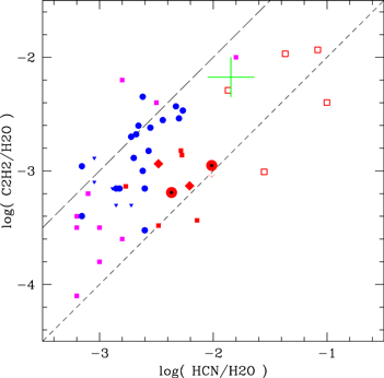
Figure 19. The Spitzer IRS spectrum of DR Tau (black) compared to the best-fit water emission spectrum (red) calculated with an LTE slab model. The adopted model parameters are T = 690 K, N ( ) = 9.3 × 1017 cm−2, and Re = 1.33 au for the radius of the projected emitting area. Emission from species other than water includes HCN at 14 μm,
  at 13.7 μm, OH (12.65, 13.07, 13.55, 14.07, 14.65 μm),
  at 15 μm, H i at 12.37 μm, and a blend of features near 12.3 μm. These features are marked in the spectrum, with asterisks marking the position of OH features. The difference between the water emission model and the observed spectrum is also shown; spectral regions that are affected by emission from other species are omitted.
Download figure:
Standard image High-resolution image
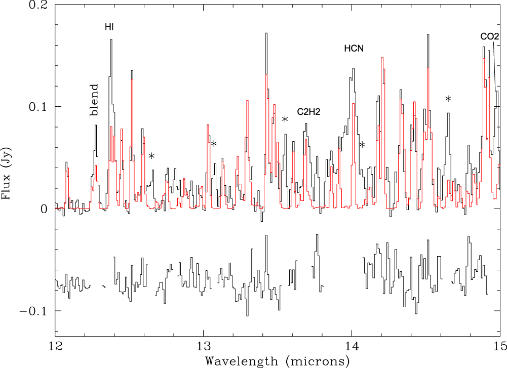
Footnotes
- 7