


Abstract
Spectral line surveys reveal rich molecular reservoirs in G331.512–0.103, a compact radio source in the center of an energetic molecular outflow. In this first work, we analyze the physical conditions of the source by means of CH3OH and CH3CN. The observations were performed with the APEX Telescope. Six different system configurations were defined to cover most of the band within (292–356) GHz; as a consequence, we detected a forest of lines toward the central core. A total of 70 lines of A/E–CH3OH and A/E–CH3CN were analyzed, including torsionally excited transitions of CH3OH ( ). In a search for all the isotopologues, we identified transitions of 13CH3OH. The physical conditions were derived considering collisional and radiative processes. We found common temperatures for each A and E symmetry of CH3OH and CH3CN; the derived column densities indicate an A/E equilibrated ratio for both tracers. The results reveal that CH3CN and CH3OH trace a hot and cold component with
  K and
K and  K, respectively. In agreement with previous ALMA observations, the models show that the emission region is compact (
 ) with gas density n(H2) = (0.7–1)×107 cm−3. The CH3OH/CH3CN abundance ratio and the evidences for prebiotic and complex organic molecules suggest a rich and active chemistry toward G331.512–0.103.
Export citation and abstract BibTeX RIS
1. Introduction
G331.512–0.103 is one of the most luminous and energetic molecular outflows known in the Galaxy. All of the system is embedded in a star-forming region known as G331.5-0.1, located in the Norma spiral arm at a distance of ∼7 pc. This source exhibits typical H ii region properties and intense maser emission of OH and CH3OH (Caswell 1998; Nyman et al. 2001; Bronfman et al. 2008). At the center of the system, a young and massive stellar object drives a bipolar flow of around 55 M⊙ with a momentum of ∼2.4 × 10³ M⊙ km s−1. Radio continuum observations have revealed a compact and central structure associated with a dust core. The central region has been also mapped with ALMA observations with transitions of SiO (8–7), H13CO+ (4–3), HCO+ (4–3) and CO (3–2). The observations revealed a ring-like structure, consistent with a cavity, and the existence of a high-velocity outflow emission confined in a region lower than 5'' in size (Merello et al. 2013a, 2013b; Hervías et al. 2015). In this work, we present new results on the emission of CH3OH and CH3CN detected toward the central core, denominated hereafter as G331.
As an interstellar laboratory, G331 exhibits active chemistry in prebiotic and complex organic molecules likely stimulated by physical processes in the molecular core and outflow. With the Atacama Pathfinder EXperiment APEX Telescope, we detected a vast number of molecular lines potentially linked to reservoirs traced by CH3OH and CH3CN. Those tracers are excellent candidates to unveil the different physical components that O- and N-bearing molecules can reveal toward hot molecular cores (Sandell et al. 1994; Wyrowski et al. 1999; Jørgensen et al. 2004; Beuther et al. 2005; Fontani et al. 2007; Fuente et al. 2014; Giannetti et al. 2017). In addition, from a chemical point of view, CH3OH and CH3CN are considered as parent and daughter molecules, respectively, in the route of interstellar molecular formation (e.g., Nomura & Millar 2004). With that motivation, we started a systematic study of G331 beginning with spectral analyses of A/E–CH3OH and A/E–CH3CN.
1.1. The Tracers CH3CN and CH3OH
CH3CN (methyl cyanide) is a symmetric top molecule. The nuclear spin state of the hydrogen atoms defines whether the molecule has an ortho (E) or para (A) symmetry. Rotational levels of CH3CN are characterized by two quantum numbers: the total angular momentum (J) and its projection on the axis of symmetry (K). Spectral signatures are associated to K-ladder structures whose notation for the A and E configurations are  and
and  , respectively (Solomon et al. 1971; Boucher et al. 1980; Cummins et al. 1983).
CH3OH (methanol) is one of the simplest asymmetric-top molecules; however, its spectrum is quite complicated because there is a strong coupling between torsional and vibrational modes. Methanol also exists in two species denoted as A and E depending on the nuclear spin alignment of the three H-atoms of the methyl group (CH3). The energy levels of methanol can be assigned with the total angular momentum J and its component K along the symmetry axis (Lees & Baker 1968; Lovas et al. 1982).
The excellent spectral resolution of the used instrument allowed us to separately study the A and E isomers of CH3CN and CH3OH. Nuclear spin conversion of A and E symmetries are considered to be rare events, being affected by chemical reactions, non-reactive collisions and grain-surface mechanisms (Willacy et al. 1993; Hugo et al. 2009). However, the spin conversion has a particular relevance in molecular astrophysics. Important questions remain unsolved: for instance, how collisions stimulate conversions and, as a consequence, if that property can be used as an astronomical clock (Lee et al. 2006; Sun et al. 2015). One of our goals is to verify if the A and E pairs are equally populated at the local temperature of the source (e.g., Andersson et al. 1984; Minh et al. 1993; Wirström et al. 2011).
We organized this paper as follows. In Section 2, the observational procedure is described. In Section 3, results about the line identification are presented. In Section 4, we discuss the radiative analysis. The discussion, conclusions, and perspectives are presented in Sections 5 and 6.
2. Observations and Methodology
The observations were carried out in 2016 March with the Atacama Pathfinder Experiment Telescope (APEX), located at Llano de Chajnantor (Chilean Andes). The spectra were obtained using the single point mode toward the coordinates R.A., decl. (J2000) = 16h12m10 1, −51°28'38
 1. We used the APEX-2 receiver of the Swedish Heterodyne Facility Instrument (SHeFI) as front end (Güsten et al. 2006; Risacher et al. 2006). The employed back end was the eXtended bandwidth Fast Fourier Transform Spectrometer2 (XFFTS2), which consists of two units with a bandwidth of 2.5 GHz divided in to 32768 channels. We selected six setups to cover a band ranging from 292 GHz to 356 GHz; they are summarized in Table 1. The integration time was estimated to obtain a conservative rms noise of ∼25 mK; then each setup expended integration times between 0.7 and 2.6 hs, with system temperatures in the range of
  K.
K.
Table 1. List of Setups Observed with the APEX-2 SHeFI Instrument Toward G331
| Setup | Frequency | Beam | Resolution |
|---|---|---|---|
| Centered at | (GHz) | ('') | (10−2 km s−1) |
| CH3CN (16–15) | 292–296 | 21.4 | 7.7 |
| CH3CN (19–18) | 329–333 | 19.0 | 6.9 |
| CH3OH (7–6) | 336–340 | 18.6 | 6.8 |
| SO (8–7) | 343–347 | 18.2 | 6.6 |
| CH3OCH3 (11–10) | 347–351 | 17.9 | 6.5 |
| HCOOCH3 (33–32) | 352–356 | 17.7 | 6.4 |
Download table as: ASCIITypeset image
The calibration was done applying the chopper-wheel technique. The output intensity provided by the system was obtained in a scale of  , which represents the antenna temperature corrected by atmospheric attenuation. The observed intensities were converted to the main-beam temperature scale using
  , the main-beam efficiency for APEX-2 (Güsten et al. 2006).
All the K-ladders structures appeared closely spaced in a wide range of frequencies so that they were observed with the same receiver. This helped us inspect irregularities due to calibration uncertainties, for which we adopted an error of 20%.
The data reduction was carried out with the CLASS package of the GILDAS software.8 The line identification was performed using the NIST9 (Lovas et al. 2009), CDMS10 (Müller et al. 2005), and JPL11 (Pickett et al. 1998) spectroscopy databases. Specifically, the CDMS and JPL catalogs were interactively loaded on the survey using the Weeds extension of CLASS. The radiative analyses were performed using the CASSIS software.12
3. Results
3.1. A/E–CH3CN
We observed the transitions CH3CN J = 16–15, J = 18–17, and J = 19–18; a set of them is displayed in Figure 1. Within those levels, the spectral resolution was high enough to separate the components K = 0, 3, 6, and 9 from K = 1, 2, 4, 5, 7 and 8, which correspond to A–CH3CN and E–CH3CN, respectively (see Table 2).

Figure 1. Lines of A/E–CH3CN and A/E–CH3OH as observed with the APEX-2 SHeFI instrument toward G331. Lines were adjusted to their rest frequencies using the CDMS and JPL catalogs. Due to the high intensity of the methanol lines, the range of the y-axis is different in both panels.
Download figure:
Standard image High-resolution imageTable 2. Spectral Line Analysis of A–CH3CN and E–CH3CN in G331
| Transition | Frequency | Eu | Aij |

|
Vlsr | FWHM |
|---|---|---|---|---|---|---|
| (MHz) | (K) | (10−3 s−1) | (K km s−1) | (km s−1) | (km s−1) | |
| A–CH3CN | ||||||
| a169–159 | 293845.164 | 697.83 | 1.51 | ⋯ | ⋯ | ⋯ |
| 166–156 | 294098.867 | 377.0721 | 1.9 | 2.065 ± 0.006 | −90.7 ± 0.2 | 10.3 ± 0.5 |
| 163–153 | 294251.461 | 184.3532 | 2.13 | 5.9 ± 0.3 | −90.4 ± 0.2 | 8.2 ± 0.6 |
| 160–150 | 294302.388 | 120.0696 | 2.21 | 7.9 ± 0.2 | −89.69 ± 0.07 | 8.8 ± 0.2 |
| b189 − 179 | 330557.569 | 728.67 | 2.36 | 0.15 ± 0.04 | −91.2 ± 0.1 | 0.9 ± 0.2 |
| c186 − 176 | 330842.762 | 407.9468 | 2.8 | 1.53 ± 0.07 | −88.2 ± 0.4 | 10 ± 0.1 |
| 183 − 173 | 331014.296 | 215.2437 | 3.07 | 6.6 ± 0.5 | −90.3 ± 0.3 | 8.9 ± 0.8 |
| 180 − 170 | 331071.544 | 150.9654 | 3.16 | 9.1 ± 0.3 | −89.5 ± 0.1 | 9.4 ± 0.3 |
| a199 − 189 | 348911.401 | 745.42 | 2.87 | ⋯ | ⋯ | ⋯ |
| 196 − 186 | 349212.311 | 424.7065 | 3.34 | 3.01 ± 0.01 | −90.4 ± 0.2 | 11.5 ± 0.5 |
| d193 − 183 | 349393.297 | 232.012 | 3.63 | 3.66 ± 0.07 | −91.7 ± 0.3 | 3.8 ± 0.6 |
| 190 − 180 | 349453.7 | 167.7368 | 3.72 | 5.5 ± 0.3 | −90.5 ± 0.1 | 6.8 ± 0.4 |
| E–CH3CN | ||||||
| e168–158 | 293940.916 | 568.69 | 1.65 | ⋯ | ⋯ | ⋯ |
| 167–157 | 294025.496 | 461.7635 | 1.78 | 0.8 ± 0.1 | −88.7 ± 0.6 | 10 ± 2 |
| 165–155 | 294161.001 | 290.5519 | 1.99 | 2.14 ± 0.09 | −89.2 ± 0.2 | 9.8 ± 0.5 |
| 164–154 | 294211.873 | 226.3073 | 2.07 | 2.93 ± 0.08 | −90.2 ± 0.1 | 9.3 ± 0.3 |
| 162–152 | 294279.75 | 140.6138 | 2.17 | 4.19 ± 0.09 | −90.79 ± 0.08 | 7.9 ± 0.2 |
| 161–151 | 294296.728 | 119.1843 | 2.2 | 7.74 ± 0.07 | −91.87 ± 0.07 | 9.4 ± 0.1 |
| f188 − 178 | 330665.206 | 599.54 | 2.52 | 1.21 ± 0.07 | −91.4 ± 0.2 | 8.1 ± 0.5 |
| 187 − 177 | 330760.284 | 492.6304 | 2.67 | 0.8 ± 0.1 | −90.8 ± 0.7 | 11 ± 2 |
| 185 − 175 | 330912.608 | 321.4329 | 2.91 | 2.9 ± 0.1 | −89.4 ± 0.2 | 11.6 ± 0.6 |
| 184 − 174 | 330969.794 | 257.1937 | 3 | 3.3 ± 0.1 | −90.5 ± 0.1 | 9.2 ± 0.4 |
| 182 − 172 | 331046.096 | 171.5073 | 3.12 | 6.66 ± 0.09 | −90.87 ± 0.07 | 10.4 ± 0.2 |
| 181 − 171 | 331065.181 | 150.0797 | 3.15 | 10.252 ± 0.007 | −91.62 ± 0.06 | 10.6 ± 0.1 |
| a198 − 188 | 349024.971 | 616.29 | 3.05 | ⋯ | ⋯ | ⋯ |
| g197 − 187 | 349125.287 | 509.38 | 3.2 | 0.304 ± 0.003 | −90.1 ± 0.6 | 5.9 ± 0.7 |
| 195 − 185 | 349286.006 | 338.1962 | 3.45 | 2.106 ± 0.008 | −89.6 ± 0.2 | 9.5 ± 0.5 |
| h194 − 184 | 349346.343 | 273.9599 | 3.55 | 2.091 ± 0.002 | −89.76 ± 0.09 | 6.1 ± 0.1 |
| 192 − 182 | 349426.85 | 188.2773 | 3.67 | 5.3 ± 0.1 | −90.61 ± 0.9 | 9.8 ± 0.2 |
| 191 − 181 | 349446.987 | 166.8506 | 3.71 | 8.018 ± 0.001 | −91.76 ± 0.05 | 9.39 ± 0.08 |
Notes. Columns 1–4 list the spectroscopic parameters collected from databases such as CDMS and JPL. Columns 5–7 contain the resulting parameters and uncertainties derived from Gaussian fits; they are line flux ( ), local standard of rest velocity (Vlsr), and the line width (FWHM). Likely blended lines with:
Download table as: ASCIITypeset image
The line identification was performed overlapping the laboratory values on the observed spectral bands at the rest velocity of the source. A high coincidence was obtained, as the K-ladder structures appeared separately and well centered, at the source's rest frequency (with Vlsr = −90 km s−1), as predicted by the spectroscopic databases (Figure 1). This inspection revealed that most of the lines have a Gaussian profile, but only a few of them presented broad blue and red wings due to the outflow activity. We applied Gaussian functions to fit and model the emission. For that, the spectral line processing was carried out using the CLASS package, by means of which we fitted baselines and Gaussian functions for each processed line. As a result, in Table 2 we listed the Gaussian fit parameters and uncertainties of each analyzed line; those parameters are the integrated line flux ( in K km s−1), local standard of rest (LSR) velocity (Vlsr in km s−1), and the line width given by the FWHM (FWHM in km s−1).
From a simple comparison of the A–CH3CN fluxes, we observed a stiff increase of them as the lines go from the K = 6 to K = 0 transitions. This behavior is in agreement with the probabilities predicted by the Einstein coefficients (Aij). For the transitions with Jup = 16, 18, and 19, the obtained patterns are 166:163: 1:3:4, 186:183:
 :4:6, and 196:193:
 1:1:2, respectively. Only few transitions diverged from this pattern, namely, A–CH3CN J = 186 − 176, and J = 193 − 183, whose emission appeared blended with HNCO (151,14 − 141,13) and C2H (
 ) at 330848 MHz and 349400 MHz, respectively. Those contaminant transitions were previously detected by Jewell et al. (1989) and Sutton et al. (1991) in Orion A and OMC-1.
For E–CH3CN lines, the derived fluxes also increase when the K-ladders vary from seven to one. This is in agreement with the spontaneous decay rates predicted by Aij. For the transitions with Jup = 16, 18, and 19, the complete patterns are 167:165:164:162: 1:2:3:5:10, 187:185:184:182:
 1:3:4:8:12, and 197:195:194:192:191 ≈1:7:7:12:26, respectively. Here, the transition E–CH3CN J = 194 − 184 at 349346 MHz appeared blended with C2H (
 ) at 349339 MHz. We also found that the transition E–CH3CN J =
  at 349125 MHz might be blended with CH3OCHO at 349124 MHz.
The search for the high levels K = 8 and K = 9 yielded negative results; we did not detect lines of these K-ladder numbers above the detection limit of the APEX data. For the cases A–CH3CN (169 − 159) and (199 − 189), we did not observe emission at all. In the case of the 189 − 179 line, we obtained a marginal flux from the Gaussian fits. This line also might be blended with c-C3HD and/or weeds,13
see Table 2. For the cases E–CH3CN (168 − 158) and (188 − 178), the emission appeared fully and partially blended with CS (6–5) and 34SO2 (212 − 211), respectively. For the 198 − 188 transition, we did not detect emission. The results are listed in Table 2. In addition, a search for emission of CH3CN ( ) was performed with the current data set; however, we did not observe clear evidences to conclude about its presence in G331.
3.2. A/E–CH3OH
As a forest of spectral lines (Figure 1), the main part of the CH3OH emission has appeared only in an interval of 3 GHz along the whole survey. The lines were identified by a simple comparison of their frequencies, corrected by the source Vlsr = −90 km s−1, with the rest frequencies reported in molecular databases. The methanol lines exhibit a symmetrical distribution which were fitted by simple Gaussian functions. The spectroscopic and fit parameters estimated for these lines are listed in Table 3. We find a FWHM of around 5.5 km s−1 and a Vlsr = −90 km s−1 with a dispersion of ±2km s−1, mainly due to lines which exhibited a low signal-to-noise ratio (S/N). In Figure 1, we show a set of A and E–CH3OH lines with J = 7–6.
Table 3. The Table 2 Caption Applies Here for A–CH3OH and E–CH3OH
| Transition | Frequency | Eu | Aij |

|
Vlsr | FWHM |
|---|---|---|---|---|---|---|
| Jk | (MHz) | (K) | (10−5 s−1) | (K km s−1) | (km s−1) | (km s−1) |
| A–CH3OH | ||||||
| 61–51 | 292672.889 | 63.707 | 10.6 | 6.95 ± 0.06 | −90.67 ± 0.02 | 5.24 ± 0.05 |
| 32–41 | 293464.055 | 51.6381 | 2.89 | 3.39 ± 0.09 | −90.35 ± 0.09 | 6.8 ± 0.2 |
| 122–113 | 329632.881 | 218.8033 | 6 | 0.59 ± 0.07 | −89.8 ± 0.3 | 4.1 ± 0.6 |
| 111–110 | 331502.319 | 169.0101 | 19.6 | 3.394 ± 0.001 | −90.17 ± 0.02 | 2.82 ± 0.03 |
| a73–81 | 332920.822 | 114.794 | 1.15 × 10⁻⁵ | ⋯ | ⋯ | ⋯ |
| 121–120 | 336865.149 | 197.0765 | 20.3 | 6.9 ± 0.5 | −91.9 ± 0.2 | 6.9 ± 0.3 |
| 70–60 | 338408.698 | 64.9817 | 17 | 10.83 ± 0.07 | −90.51 ± 0.02 | 5.31 ± 0.04 |
| 76–66 | 338442.367 | 258.6994 | 4.53 | 1.09 ± 0.06 | −91.3 ± 0.1 | 5.7 ± 0.4 |
| 75–65 | 338486.322 | 202.8864 | 8.38 | 2.11 ± 0.08 | −90.98 ± 0.09 | 4.9 ± 0.2 |
| 72–62 | 338512.853 | 102.7032 | 15.7 | 7.3 ± 0.4 | −90.5 ± 0.1 | 5.5 ± 0.4 |
| 73–63 | 338543.152 | 114.7948 | 13.9 | 9.21 ± 0.08 | −89.77 ± 0.02 | 5.62 ± 0.05 |
| 72–62 | 338639.802 | 102.7179 | 15.7 | 7.4 ± 0.7 | −90.6 ± 0.2 | 5.6 ± 0.6 |
| 22–31 | 340141.143 | 44.6729 | 2.79 | 2.14 ± 0.06 | −90.71 ± 0.08 | 5.5 ± 0.2 |
| a161–152 | 345903.916 | 332.6545 | 9.02 | ⋯ | ⋯ | ⋯ |
| 54–63 | 346204.271 | 115.1625 | 2.17 | 2.31 ± 0.07 | −90.74 ± 0.09 | 5.9 ± 0.2 |
| 141 − 140 | 349106.997 | 260.2068 | 22 | 4.25 ± 0.06 | −90.77 ± 0.04 | 5.41 ± 0.09 |
| 11–00 | 350905.1 | 16.841 | 33.1 | 12.19 ± 0.05 | −90.58 ± 0.01 | 5.13 ± 0.03 |
| a82–90 | 351685.48 | 121.2915 | 16.2 | ⋯ | ⋯ | ⋯ |
| a104–112 | 355279.539 | 207.9929 | 1.22 × 10⁻³ | ⋯ | ⋯ | ⋯ |
| 130–121 | 355602.945 | 211.0285 | 12.6 | 4.02 ± 0.04 | −91.01 ± 0.02 | 4.76 ± 0.06 |
| 151–150 | 356007.235 | 295.2675 | 23 | 2.68 ± 0.05 | −90.46 ± 0.05 | 5.8 ± 0.1 |
| E–CH3OH | ||||||
| 8−3–9−2 | 330793.887 | 138.3774 | 5.38 | 1.96 ± 0.06 | −91.03 ± 0.07 | 4.6 ± 0.1 |
| 16−1–15−2 | 331220.371 | 312.7333 | 5.23 | 0.55 ± 0.06 | −91.4 ± 0.3 | 5.3 ± 0.6 |
| 33–42 | 337135.853 | 53.7412 | 1.58 | 1.09 ± 0.06 | −91.1 ± 0.1 | 4.7 ± 0.3 |
| a72–62 | 337671.238 | 456.8285 | 15.5 | ⋯ | ⋯ | ⋯ |
| a75–65 | 337685.248 | 486.0568 | 8.28 | ⋯ | ⋯ | ⋯ |
| a7−1–6−1 | 337707.568 | 470.3161 | 16.5 | ⋯ | ⋯ | ⋯ |
| 70–60 | 338124.488 | 70.1794 | 16.9 | 9.09 ± 0.06 | −90.74 ± 0.01 | 5.01 ± 0.04 |
| 7−1–6−1 | 338344.588 | 62.6521 | 16.6 | 9.61 ± 0.08 | −90.63 ± 0.02 | 4.87 ± 0.05 |
| a76–66 | 338404.61 | 235.8941 | 4.51 | ⋯ | ⋯ | ⋯ |
| a7−6–6−6 | 338430.975 | 246.0504 | 4.54 | ⋯ | ⋯ | ⋯ |
| 7−5–6−5 | 338456.536 | 181.1017 | 8.34 | 1.3 ± 0.4 | −90.9 ± 0.7 | 5 ± 2 |
| 75–65 | 338475.226 | 193.1625 | 8.34 | 1.5 ± 0.6 | −91 ± 0.1 | 5 ± 3 |
| 7−4–6−4 | 338504.065 | 144.9961 | 11.5 | 4 ± 2 | −91.3 ± 0.04 | 6 ± 1 |
| 74–64 | 338530.257 | 153.0934 | 11.5 | 3.1 ± 0.6 | −91.1 ± 0.4 | 5 ± 1 |
| 7−3–6−3 | 338559.963 | 119.8084 | 14 | 4.5 ± 0.1 | −90.93 ± 0.6 | 5.2 ± 0.1 |
| 73–63 | 338583.216 | 104.8115 | 13.9 | 6.9 ± 0.2 | −90.99 ± 0.08 | 6.6 ± 0.2 |
| 71–61 | 338614.936 | 78.1537 | 17.1 | 21.4 ± 0.8 | −89.5 ± 0.2 | 9.9 ± 0.5 |
| 7−2–6−2 | 338722.898 | 83.0148 | 15.7 | 12.53 ± 0.07 | −90.04 ± 0.01 | 5.61 ± 0.03 |
| a182−173 | 344109.039 | 411.5062 | 6.79 | ⋯ | ⋯ | ⋯ |
Note.
aMarginal emission ( ).
).
Download table as: ASCIITypeset image
Although most of the methanol emission corresponds to the torsional ground state, we also identified lines corresponding to the first excited state ( ). Such is the case for the lines displayed in Figure 2 (upper panel), where it is observed a broad line of 34SO at ∼337580 MHz blended with the transition E–CH3OH (
 )
)  at a frequency, corrected by the source Vlsr, of 337581.663 MHz. Around the 34SO peak, minor satellite emission also was identified as corresponding to (A/E)-CH3OH
  the spectroscopic parameters are summarized in Table 4. In the bottom panel of Figure 2, we display the only excited line without contaminant emission, which corresponds to A–CH3OH (
 )
)  at a frequency, corrected by the source Vlsr, of 337969.414 MHz.

Figure 2. Panels showing the torsional excited lines of A–CH3OH (red dashed–dotted line) and E–CH3OH (blue dashed line) against the spectra of G331 (black histogram). In increasing order, the Gaussian fits are centered at the rest frequencies ∼337546 MHz, 337581 MHz (blended with 34SO), 337605 MHz, 337625 MHz, 337635 MHz, 337643 MHz, and 337969 MHz.
Download figure:
Standard image High-resolution imageTable 4.
The Table 2 Caption Applies Here for A–CH3OH  and E–CH3OH
| Transition | Frequency | Eu | Aij |

|
Vlsr | FWHM |
|---|---|---|---|---|---|---|
| Jk | (MHz) | (K) | (10−5 s−1) | (K km s−1) | (km s−1) | (km s−1) |
A–CH3OH 
|
||||||
| a75–65 | 337546.048 | 485.4 | 8.13 | 1.047 ± 0.004 | −92.8 ± 0.3 | 9.1 ± 0.5 |
| a72–62 | 337625.679 | 363.5 | 15.5 | 10.2 ± 0.9 | −90.5 ± 0.3 | 8 ± 1 |
| a72–62 | 337635.655 | 363.5 | 15.5 | 1.2 ± 0.2 | −92.6 ± 0.6 | 9 ± 2 |
| 71–61 | 337969.414 | 390.1 | 16.6 | 0.39 ± 0.05 | −90.8 ± 0.3 | 5.2 ± 0.7 |
E–CH3OH 
|
||||||
| a74–64 | 337581.663 | 428.2 | 11.3 | ⋯ | ⋯ | ⋯ |
| a7−2–6−2 | 337605.255 | 429.4 | 15.6 | 1.513 ± 0.003 | −89.8 ± 0.3 | 11.7 ± 0.5 |
| a70–60 | 337643.864 | 365.4 | 16.9 | 1.1 ± 0.8 | −90.2 ± 0.2 | 5.9 ± 0.5 |
| b10−2–11−3 | 344312.267 | 491.91 | 17.7 | ⋯ | ⋯ | ⋯ |
Note. Transitions and quantum numbers from Xu & Lovas (1997) and references therein. Likely blended lines with:
a34SO 88–77 (337580 MHz). bSO 88–77 (344310 MHz).Download table as: ASCIITypeset image
Emission of excited methanol is typically observed toward hot molecular cores. For instance, Menten et al. (1986), Sutton et al. (1995) and Schilke et al. (2001) have reported its emission in OMC-1, W3(OH), and W51.
The observed lines of excited methanol constitute an evidence for its presence in G331. However, to solve questions as whether the excited emission is populated at the same conditions of the ground state, it is necessary to carry out complementary observations; for instance, at frequencies between 600–720 GHz. These observations could reveal a larger number of CH3OH  lines favoring a better estimation on the physical conditions. In the bottom panel of Figure 2, we displayed a broad line close to 337900 MHz, which is associated to SO2; however, that line could be also blended with CH3OH (
 ) J = 7–6 at 337877 MHz.
3.3. Isotopologues
We searched for lines of the D, 13C, 15N and 18O isotopologues of CH3CN and CH3OH. As predicted by the spectroscopic databases, several frequencies of those isotopologues fall across the bands; however we only confirm the presence of 13CH3OH. Emission related to 13CH3CN J = 19–18 was also identified; however, the lines are blended with SO J = 3–2 at 339341 MHz. Those lines were also reported by Jewell et al. (1989) in Orion A.
We detected a couple of transitions of A–13CH3OH. The associated spectroscopic parameters are presented in Table 5. The lines were identified at the rest frequencies 330252.798 MHz and 350103.118 MHz with S/N of  . Such detections have been fundamental to analyze the opacity of the detected emission. For instance, we estimated flux ratios using lines of A–13CH3OH and A–CH3OH with comparable spectroscopy, namely using those transitions that have exhibited similar frequencies, Aij and Eu values. Then, by selecting the
  –
– and
and  –
– transitions both of A–CH3OH and A–13CH3OH (Tables 3 and 5), whose Aij values are in agreement almost by a factor 1, we obtained the flux ratios C/13C = 18.1 ± 0.7 and C/13C = 17.7 ± 0.1, respectively. Such flux ratios are similar to the values reported in sources toward the Galactic center, where C/13C = 20 (Wilson & Rood 1994; Requena-Torres et al. 2006). These ratios imply finite values of opacities, therefore in the subsequent sections we will take into account optical depth corrections to estimate the physical conditions derived from the CH3OH and CH3CN emission.
Table 5.
Spectroscopic and Observational Parameters of the of the  CH3OH Lines Analyzed in G331
| Transition | Frequency | Eu | Aij |

|
Vlsr | FWHM | aC/13C |
|---|---|---|---|---|---|---|---|
| Jk | (MHz) | (K) | (10−5 s−1) | (K km s−1) | (km s−1) | (km s−1) | |
| 70–60 | 330252.798 | 63.4 | 15.8 | 0.60 ± 0.07 | −90.7 ± 0.3 | 5.0 ± 0.6 | 18.1 ± 0.7 |
| 11–00 | 350103.118 | 16.8 | 32.9 | 0.69 ± 0.05 | −91.2 ± 0.2 | 4.3 ± 0.3 | 17.7 ± 0.1 |
Note. Similarly, the Table 2 caption applies here.
aFlux ratios derived by considering the integrated fluxes of A–CH3OH (70–60) and (10–00) listed in Table 3.Download table as: ASCIITypeset image
Two lines of E–13CH3OH were also identified, although they exhibited contamination. Close to their rest frequencies, lines of 34SO2 J = 8–7 and CH3OCH3 J = 16–15 are candidates for blended emission. These contaminants were also detected toward the Hot Molecular Core G34.3+0.15 (MacDonald et al. 1996).
4. Physical Conditions
4.1. Statistical Equilibrium Calculations
In this section, we present results based on statistical equilibrium models when considering collisions between the analyzed molecules and molecular hydrogen. To estimate the kinetic temperatures and column densities, we ran the RADEX code into CASSIS, whose formalism is analogous to the Large Velocity Gradient approximation (van der Tak et al. 2007). RADEX considers the probability that a photon escape in an isothermal and homogeneous medium without large-scale velocity fields. Collision rate data were collected from the LAMDA database.14
Conjointly with RADEX/CASSIS, we used the Markov Chain Monte Carlo (MCMC) method to simulate the observed lines from the resulting best solutions, which are given by the minimal  value. The MCMC algorithm operates on values chosen randomly within a sample defined by a minimum and maximum limit for an N-dimensional parameter space. This characteristic is the most relevant when calculations require as inputs several free parameters. In detriment, the quality of the fit is a monotonically increasing function of the number of iterations introduced in the chain, which in turn affects the "computational time" to achieve convergence (e.g., Guan & Krone 2007; Foreman-Mackey et al. 2013; Tahani et al. 2016).
We prepared MCMC routines for each A and E species. The numerical sample explored by the algorithm was delimited by five free parameters: kinetic temperature (Tk), column density (N), source size (θ), FWHM and hydrogen density ( ). To guarantee that the code has visited the sample, we tested routines with number of iterations of the order of 105. Once the algorithm achieves convergence, the minimal
  is computed printing the statistical results for each parameter. This methodology implied large run-times. As a total, we modeled seven and 13 lines of A–CH3CN and E–CH3CN, respectively, and 10 and 13 lines of A–CH3OH and E–CH3OH, respectively. The statistical calculations are summarized in Table 6. Likewise, the best-fit model lines are exhibited in Figure 3.

Figure 3. Spectral lines and the best fits assuming non-LTE conditions, plotted as a function of the frequency corrected by the source Vlsr, of (a) A–CH3CN (blue dashed line) and E–CH3CN (red dashed–dotted-line) and (b) A–CH3OH (blue dashed line) and E–CH3OH (red dashed–dotted-line). For A/E–CH3CN, the models yielded a kinetic temperature between ∼(140–142) K and column densities between ∼(3.7–4.8) × 1014 cm−2. For A/E–CH3OH, the models yielded a kinetic temperature between ∼(64–85) K and column densities between ∼(8.5–9.8) × 1015 cm−2.
Download figure:
Standard image High-resolution imageTable 6. Parameters and Physical Conditions Derived from the Statistical Equilibrium Calculations that have Yielded Hydrogen Densities between 0.7 and 1 × 107 cm−3
| Parameters | A–CH3CN | E–CH3CN | A–CH3OH | E–CH3OH |
|---|---|---|---|---|
| Modeled lines | 7 | 13 | 10 | 13 |

|
5.69 | 7.77 | 6.23 | 4.42 |
| FWHM (km s−1) | 5.49 ± 0.01 | 5.49 ± 0.01 | 4.9 ± 0.1 | 4.88 ± 0.01 |
| N (1014 cm−2) | 4.77 ± 0.05 | 3.69 ± 0.04 | 85 ± 20 | 98 ± 0.1 |
| Tk (K) | 142.1 ± 0.9 | 140.5 ± 0.3 | 64 ± 2 | 84.8 ± 0.1 |
| θ ('') | 4.51 ± 0.01 | 4.53 ± 0.02 | 5.7 ± 0.3 | 5.01 ± 0.04 |
Note. The number of computed lines and the reduced  values have also been included.
Download table as: ASCIITypeset image
There are two aspects that were common for the models of A/E–CH3OH and A/E–CH3CN. First, we obtained H2 densities in the interval  cm−3, which is in agreement within a factor ≳1.5 with the density derived from the dust continuum (Hervías-Caimapo et al. submitted). Also, we intended to differentiate the densities of the ortho-H2 and para-H2 collisional partners (o-H2 and p-H2, respectively). Although studies explain the differences when A and E species collide with o-H2 and p-H2 (e.g., Rabli & Flower 2010), for our purposes we just conclude that the o-H2/p-H2 ratio varied between ∼0.6 and 1.0 for the different MCMC computations. That interval is consistent with the ortho-to-para limit of 0.2, when H2 is thermalized at the CO temperature, and ortho-to-para limit of three when H2 first forms (Flower & Watt 1984; Lacy et al. 1994).
The second aspect is that the modeled spectral lines yielded source sizes in agreement with a compact emitter region. For CH3CN and CH3OH we found sizes of ∼45 and ∼53, respectively. This result is supported by previous CO (7–6) maps obtained with the Australia Telescope Compact Array (ATCA), for which Bronfman et al. (2008) determined a compact and dense region of ∼43. Merello et al. (2013a, 2013b) mapping the emission traced by SiO (8–7) found a ring-type structure of ≲5''.
4.2. LTE Analysis
Rotational diagrams were constructed to estimate the excitation temperatures (Texc) and column densities (N) of A/E–CH3CN and A/E–CH3OH. Assuming that the emission is optically thin and uniformly fills the antenna beam, Texc and N can be calculated from

where  and Eu are the column density per statistical weight and the energy of the upper level, respectively, and Z is the partition function (Goldsmith & Langer 1999). In local thermodynamic equilibrium (LTE), Equation (1) represents a Boltzmann distribution whose values
  versus
  can be fitted using a straight line, whose slope is defined by the term
  .
.
The rotational diagrams were constructed taking a beam dilution factor associated with a point-like emitter region. Therefore, a correction that is provided by the term  was introduced on the right-hand side of Equation (1) (Goldsmith & Langer 1999). This ratio relates the subtended angle of the source with the solid angle of the antenna beam. The beam dilution factor that we introduced is based on the results derived from the RADEX/MCMC calculations. Then, for CH3CN and CH3OH, we adopted averaged source sizes of 45 and 53, respectively.
Because the lines observed in this work fell in a broad band, from 290 to 350 GHz, yielding different beamwidths, the adopted sizes have been used in the comparisons between temperatures and column densities for the different lines.
Depending on the density of the region, the K-ladder structures of CH3CN and CH3OH can exhibit an important scattering of ( ) values in their rotational diagrams. More generally, it is expected that the higher is the gas density, the lower is the K-ladder segregation (Olmi et al. 1993; Cesaroni et al. 1997; Goldsmith & Langer 1999; Remijan et al. 2004; Araya et al. 2005; Cuadrado et al. 2017). To check the amount of scatter, we compared the rotational diagrams when they were individually constructed for each JK level and with those obtained when an unique fit was determined across all the K-levels. As a result, we did not observe considerable discrepancies between the two cases; temperatures and column densities were found within the adopted uncertainty from calibration (Section 2). For instance, in Figure 4 we display the result for E–CH3CN.

Figure 4. Rotational diagram fits of E–CH3CN across all the K-ladder levels (dashed-dotted line), yielding  7.5 × 1014 cm−2 and
  172 K, and within each K-ladder structure for the transitions J = 16–15 (black triangles), J = 18–17 (red squares), and J = 19–18 (blue pentagons).
Download figure:
Standard image High-resolution imageOptical Depth Correction
The rotational diagrams obtained from the A/E–CH3CN and A/E–CH3OH lines are displayed in Figure 5. They were constructed selecting only the transitions in the ground state and without contaminant emission. So far, the rotational diagrams have been scaled only considering the beam dilution factor. However, they represent a solution under the assumption of emission optically thin,  . To revise how different the LTE solutions are from a radiative scenario with finite values of optical depths, we have applied an optical depth correction on the rotational diagrams of A/E–CH3CN and A/E–CH3OH. Expressed mathematically, the correction consisted in including the term
  , with
  , on the right-hand side of Equation (1) (Goldsmith & Langer 1999; Gibb et al. 2000; Remijan et al. 2004; Araya et al. 2005). Thus, the ordinates of our rotational diagrams were readjusted considering a term associated with the photon escape probability.

Figure 5. Upper panels: rotational diagrams of A–CH3CN and E–CH3CN showing the least-square fits with the optical depth correction, represented with the asterisk symbols and dashed-dotted lines, and without the optical depth correction, represented with the filled triangles and solid lines. Bottom panels: the same as above for A–CH3OH and E–CH3OH. Column densities and excitation temperatures correspond to the results when applied the optical depth correction, numbers in parenthesis represent uncertainties on the last digit.
Download figure:
Standard image High-resolution imageWe have performed this adjust based on (first) the results obtained from the statistical equilibrium calculations. In the case of CH3CN, transitions with K = 0, 1, 2 and 3 were the most affected with  . And, (second) considering the flux ratio C/13C ≲ 20 as we described in Section 3.3, which suggests finite optical depths.
To perform the optical depth correction, we used CASSIS which executes iterative calculations of  adjusting the level populations until achieving a consistent solution. With these corrections, slight changes are expected in the LTE solutions. For instance, Araya et al. (2005) obtained differences around 10 and 14% in the temperature and column density of CH3CN when the optical depth correction was applied, respectively.
The A/E–CH3CN rotational diagrams (RDs), with the optical depth correction, are displayed in the upper panels of Figure 5. For A–CH3CN, we obtained N = (6.4 ± 2.0) × 1014 cm−2 and Texc = 156 ± 25 K. For E–CH3CN, we obtained N = (8.4 ± 2.0) × 1014 cm−2 and Texc = 152 ± 20 K. The percentage difference of N and Texc, with respect to the RD without the optical depth correction, are ranged between (5–14)% and (2–12)%, respectively.
The A/E–CH3OH RDs, with the optical depth correction, are displayed in the lower panels of Figure 5. For A–CH3OH, we obtained N = (1.9 ± 0.5) × 1016 cm−2 and Texc = 71 ± 10 K. For E–CH3OH, we obtained N = (2.0 ± 0.1) × 1016 cm−2 and Texc = 68 ± 8 K. The percentage difference of N and Texc, with respect to the RD without the optical depth correction, are ranged between (10–22)% and (9–17)%, respectively.
We detected two lines of 13CH3OH (Table 5). In the absence of collisional coefficients, those lines were modeled assuming LTE conditions applying the MCMC method leaving various inputs as free parameters: N, Texc, FWHM, and θ. However, we put an upper limit of  5 × 1015 cm−2, which was derived from the column density of the main isotopologue and considering the ratio C/13C ≲ 20. The results were consistent with the physical conditions of the main isotopologue. The best LTE models are displayed in Figure 6, whose solution (
 ) yielded N = (1.01 ± 0.06) × 1015 cm−2 and Texc = 89.5 ± 0.4 K for a modeled source size of 57. Additionally, the resulting FWHM values (∼4.4 km s−1) are consistent with the resulting fits reported in Table 5.

Figure 6. Spectral lines and LTE models of A–13CH3OH represented by black histograms and Gaussian curves, respectively. Lines  –
– and
and  –
– appeared at the rest frequencies 330252.798 MHz and 350103.118 MHz, respectively. The models were derived from a computation whose best solution provided N = (1.01 ± 0.06)×1015 cm−2 and Texc = 89.5 ± 0.4 K.
Download figure:
Standard image High-resolution image5. Discussion
5.1. Molecular Abundances
CH3OH is more abundant and traces a region about 70 K colder than that traced by CH3CN. From the LTE and non-LTE analysis, we found that the ratio (A + E)-CH3OH/(A + E)-CH3CN is about 25, indicating almost the same overabundance of A and E–CH3OH over A–CH3CN and E–CH3CN.
ALMA observations of the ion H13CO+ (4–3) probed the existence of a core and various clumpy structures in G331 (Hervías-Caimapo et al. submitted). Maps of SiO (8–7) show as well an internal cavity surrounded by molecular emission confined in ≲5'', for which these authors have estimated N(H13CO+) ≈ (1.5–3) ×1013 cm−2 (e.g., Bronfman et al. 2008; Merello et al. 2013a, 2013b). The column densities of CH3OH and CH3CN were divided by N(H2) values to obtain their abundances. Following the works cited above, to estimate a scaled density of H2 in G331, we applied the ratio H13CO+/H2 = 3.3 × 10⁻¹¹ of Orion KL (e.g., Blake et al. 1987) on the H13CO+ column densities derived for G331 (Merello et al. 2013a). As an approximation for the present work, we adopted the H13CO+/H2 ratio of the Orion KL system, as this source is an excellent template for comparative studies on abundances and molecular complexity (e.g., Schilke et al. 2001; Beuther et al. 2005). The total abundances of CH3OH and CH3CN are summarized in Table 7; as a total, we refer to the A+E contribution from the nuclear spin symmetries (e.g., Fuente et al. 2014 ). Thus, the CH3CN emission is linked to a hot core with  K and
K and  , while CH3OH traces a cold bulk medium with
  K and
K and  . Also in Table 7, we included the abundance uncertainties computed from the errors obtained with the radiative models (Bevington & Robinson 2003); although we listed errors of ≲25%, the abundance uncertainties could be of up to 40% including other sources of errors, such as the calibration uncertainty, adopted here as 20%. In Table 7, the abundances of the 13C isotopologues are also listed. Although we obtained an inaccurate result based only on two lines of 13CH3OH, we found that it could be not only 20 times lower, resulting from the 13C/C flux ratio, but up to 40 times under abundant than CH3OH, as the LTE analysis suggested (see Figure 6). Thus, we determined [13CH3OH] ≲ 2.1 × 10⁻⁹.
Table 7. Abundances of CH3OH and CH3CN Derived from the LTE and Non-LTE Analysis
| Method | Hot Component | Cold Component | ||||
|---|---|---|---|---|---|---|
| [CH3CN] | [13CH3CN] |

|
[CH3OH] | [13CH3OH] |

|
|
| 10−9 | 10−9 |

|
10−9 | 10−9 |

|
|
| non-LTE | 1.8 ± 0.2 | ⋯ | 56 | 38 ± 10 | ⋯ | 46 |
| LTE | 3.1 ± 0.6 |

|
43 | 81 ± 15 |

|
49 |
Note. We have included the contribution of each spin isomer as a percentage of the total abundance, assumed as the sum A+E of the symmetries.
Download table as: ASCIITypeset image
For the undetected 13CH3CN, we propose upper limits assuming that the 13CH3CN/13CH3OH ratio works as what we found for the main isotopologues: CH3CN/CH3OH  . From that conjecture, we conclude that [13CH3CN] ≲ 8 × 10⁻¹¹.
One of the goals of this work was to separately analyze the emission of the A and E spin nuclear isomers; however, the analysis indicated common physical conditions (N and T) for both spin symmetries meaning that they trace the same reservoir. The opposite case would imply spin conversion processes, induced by molecular interactions on molecular ices or collisions in gas phase, favoring an overabundance in a given spin symmetry. However, this result would be expected at earlier stages or in younger stellar sources (e.g., Minh et al. 1993; Wirström et al. 2011).
Independent of the employed analysis, we find that both the A and E isomers contribute with approximately half of the total emission of CH3OH and CH3CN. The percentage derived from both methods are listed in Table 7, as explained above, assuming a total abundance as A+E. As a similar result, MacDonald et al. (1996) determined the ratio [A–CH3OH]/[E–CH3OH] ≈ 0.9 for the hot molecular core G34.3+0.15. In the envelopes around low-mass protostars, Jørgensen et al. (2005) found ortho-to-para ratios close to unity for CH3OH. Recently, similar results were reported for the pairs A/E–CH3CN, A/E–CH3OH, and A/E–CH3CHO in the Orion Bar photodissociation region (PDR; Cuadrado et al. 2017).
This tendency is similar to another aspect aimed to examine in this study: whether o- and p-H2 collisional partners may affect the population of the A and E nuclear spin isomers of CH3OH and CH3CN. However, the MCMC/RADEX computations yielded H2 ortho-to-para ratios close to unity.
Laboratory studies have offered new measurements about spin conversion, generally assumed as improbable processes. In gas phase, Sun et al. (2015) found that molecular collisions induce the interconversion of spin in molecules of methanol exhibiting a rate that decreases as the pressure increases with the number of collisions. A quantum relaxation mechanism explains the interconversion. In condensed phase, Lee et al. (2006) observed that methanol can suffer a slow conversion from the E to the A symmetry when it is trapped in a solid matrix of p-H2 prepared at low temperatures (∼ 5 K). In theoretical works, Rabli & Flower (2010) studied the implications of methanol colliding with o-H2 and p-H2, finding qualitative and quantitative differences for those cases.
As we summarized in Table 4, emission of torsionally excited methanol was also evidenced; however, only one line appeared without blended emission: A–CH3OH ( ) at ∼337969 MHz. In some studies, it has been analyzed whether excited transitions may be populated at the same LTE conditions of the ground torsional levels (e.g., Lovas et al. 1982; Menten et al. 1986; Sutton et al. 1995; Ren et al. 2011; Sánchez-Monge et al. 2014). We made a minor examination based on the unique line without contamination; however, we found that, to account for the flux, different regimes are needed with
  K. Complementary observations with APEX will be carried out to determine with a better precision the physical conditions of excited methanol in G331.
5.2. The Hot and Cold Components of G331
In this study, we identified two different components that could candidate G331 as a Hot Molecular Core (HMC). Other characteristics also support this hypothesis. For instance, the source is compact, harbors a massive and energetic molecular outflow, and is embedded in a H ii region where masers of OH and CH3OH reveal a high star formation activity. Besides, the temperatures of the gas components are above and below the limits where evaporation of icy mantles plays an important role; for instance, to explain abundances of Complex Organic Molecules and aspects related to the age of the source. The gas densities also support such classification, since we determined H2 densities typical of a dense medium (0.7–1)  cm−3.
cm−3.
N- and O-bearing molecules help to diagnose the presence of different gas components in HMCs (e.g., Beuther & Sridharan 2007; Fontani et al. 2007). In this first work, it is proposed that A/E–CH3CN and A/E–CH3OH trace a hot ( K) and cold (
 K) component with sizes around 45 and 53, respectively. Such results are in agreement with ALMA observations of CO (7–6), SiO (8–7) and H13CO+ (4–3). The emission of these species was found to be compacted in ∼5'' (Bronfman et al. 2008; Merello et al. 2013a; Hervías et al. 2015).
In Figure 7, we compare the abundances derived in this work with other sources. Our results are similar with the abundances reported in G34.3+0.15. More generally, our results suggest different abundances, physical components, and a chemical differentiation for CH3OH and CH3CN in G331. The high sensitivity and spectral resolution of our single-dish spectra have been useful to realize subtle differences in the line profiles of CH3OH and CH3CN, inspected via the Vlsr and FWHM parameters listed in Tables 2 and 3. In agreement with the radiative models, these spectral signatures reveal clues on the origin and size of the emitter regions. In spite of that, and as a perspective, further observations at higher spatial resolution are needed to study the spatial distribution of different tracers in G331. Also, these observations may reveal density gradients toward the core and the outflow, allowing more accurate determinations of molecular abundances.

Figure 7. Comparison of the abundances of CH3OH (red) and CH3CN (black) in hot molecular cores, clouds, and PDR regions. Values were collected from references such as Sutton et al. (1995), MacDonald et al. (1996), Helmich & van Dishoeck (1997), Gibb et al. (2000), Nummelin et al. (2000), Jørgensen et al. (2005), Ren et al. (2011), Crockett et al. (2014), and Cuadrado et al. (2017).
Download figure:
Standard image High-resolution image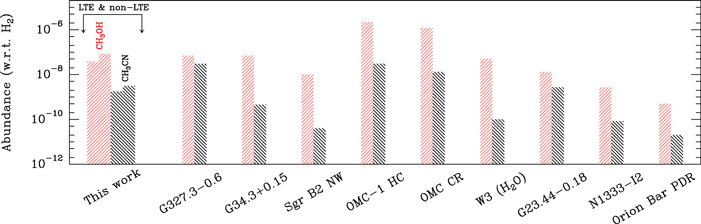
The fact of CH3OH being more abundant than CH3CN is in agreement with the chemistry that has been modeled in HMCs, where these molecules are usually referred as parent and daughter species, respectively, since CH3OH is expected to be formed at early stages in grain surfaces, via successive hydrogenation of CO, while CH3CN appears later via reaction between HCN and  (Millar et al. 1997; Nomura & Millar 2004; Guzmán et al. 2013; Loison et al. 2014). Other alternatives to produce methanol are
  + OH
+ OH  CH3OH and CH2 + H2O
  CH3OH. They can occur when frozen mixtures of CH4 and H2O are bombarded with electrons (Hiraoka et al. 2006). In addition, we have found that the physical conditions traced by those molecules might explain the regimes where prebiotic and complex organic molecules have been detected, such as CH3OCH3, CH3CHO, NH2CHO, and the C2H4O2 isomers.
Nomura & Millar (2004) performed time-dependent chemical models considering observational aspects of the hot molecular core G34.3+0.15; for instance, that CH3CN is associated to an inner and hot core region, while CH3OH traces the gas present in clumps (e.g., Hatchell et al. 1998; Millar & Hatchell 1998; van der Tak et al. 2000). Comparing our column densities with the temporal values calculated by those authors, an age of 104 years may represent the epoch for G331, when substantial quantities of daughters molecules (e.g., CH3CN) are produced without substantially decimate their parents (e.g., CH3OH). Preliminary results derived by us, obtained with the gas-grain chemical code Nautilus (Ruaud et al. 2016),15 show a CH3OH/CH3CN ratio similar to those derived from the observations. However, these results will be presented in a subsequent work depicting the chemistry of O-bearing molecules detected in the source.
6. Conclusions and Perspectives
As an active interstellar laboratory, the G331.512–0.103 system exhibits a rich chemistry in organic and prebiotic molecules. In this first article, we analyzed around 70 lines of A/E–CH3OH and A/E–CH3CN toward the central region, abbreviated here as G331. Torsionally excited transitions of methanol were evidenced. Without contaminant emission, we identified the CH3OH ( )
)  –
– transition. Likewise, two lines corresponding to 13CH3OH were detected at 330252.798 MHz and 350103.118 MHz.
The analyses were performed including collisions with H2 and typical radiative processes under LTE conditions, namely rotational diagrams. Both analyses coincide in that CH3OH traces a cold component, while CH3CN traces a hotter core with kinetic temperatures of ∼74 K and 141 K, respectively. Likewise, the best-fits indicated emitter regions of around 45 and 53 for these tracers, respectively, with gas density n(H2) = (0.7–1) × 107 cm−3.
We treated independently each one of the nuclear spin isomers of CH3OH and CH3CN, and determined the ratio (A + E)-CH3OH/(A + E)-CH3CN ≃ 25. The temperatures and densities of each A and E pair suggest that they trace a same bulk and are equally populated at each local temperature. Considering that, we estimated the CH3OH and CH3CN abundances from the total contribution A+E. Under the LTE formalism, we estimated that [CH3OH]  , [CH3CN]
  , and the upper limits [13CH3OH]
  and [13CH3CN]
  .
.
Under the perspective of hot molecular cores, the CH3OH/CH3CN ratio could be associated with and epoch between (104–105) years, when daughter molecules like CH3CN start to be produced from parent molecules, such as CH3OH.
We thank the anonymous referee for constructive comments and suggestions on the paper. We thank the APEX staff for their helping during the observations. N.U.D. acknowledges support from CONICET, projects PIP 00356, and from UNLP, projects 11G/120 and PPID/G002. L.B., R.F., and N.R. acknowledge support from CONICYT project BASAL PFB-06. E.M. and J.R.D.L. acknowledge support from the grant 2014/22095-6, São Paulo Research Foundation (FAPESP).
Facilities: Atacama Pathfinder EXperiment - , APEX telescope. -
Software: CASSIS (http://cassis.irap.omp.eu/), GILDAS (https://www.iram.fr/IRAMFR/GILDAS/), RADEX (http://doi.org/10.1051/0004-6361:20066820) NAUTILUS (https://doi.org/10.1093/mnras/stw887).
Footnotes
- 8
- 9
- 10
- 11
- 12
- a
Marginal emission (<5σ).
- 13
Conventional term adopted to label species with numerous spectral lines in the mm/sub-mm regime.
- 14
Leiden Atomic and Molecular Database LAMDA, http://home.strw.leidenuniv.nl/moldata/.
- 15