A temporally and spatially local spike-based backpropagation algorithm to enable training in hardware

We propose a composite spiking neuron that can simultaneously compute both the feedforward spikes and the backpropagated gradient spikes with positive and negative streams as the fundamental unit of our network. Further, we introduce an approximation of the softmax cross-entropy loss implemented using inhibitory lateral connections to enforce WTA in the output layer. For stable learning and regularization in our experiments, we also adopt the He weight initialization scheme [28] and dropout [29] respectively.

We use a Spike Response kernel method [14] to perform efficient GPU-compatible simulations of our spiking network. In this method, the incoming spike trains at any neuron are convolved with a spike response kernel, which converts weighted discrete delta-function spikes into their corresponding PSPs and accumulates their values over time. This convolution operation, then, computes the membrane potential of the neuron across the simulation time in one shot and is followed by a thresholding operation to generate the spike train from the computed membrane potential. Due to the one-shot computation of neuron membrane potential in the kernel method, the thresholding operation is slightly different from the standard issue spike-and-reset method of simulations that compute the membrane potentials at every time step in sequence. Since the membrane potentials are pre-computed without resetting, we have to instead, increment the threshold after every spike is issued. In doing this, we are making use of the fact that for a spiking threshold of θ, spikes should be issued at the time instances when the pre-computed membrane potential (computed without any spike-issue resetting) crosses θ, 2θ, 3θ and so on.

Additionally, since the membrane potential of any neuron is computed in one shot from known input spikes to that neuron and the thresholding and spike-generation operation occur separately, this method cannot directly implement lateral connections, which are required in our final layer. To solve this problem, we have used an iterative approach where at any given iteration, we use the available spikes of the same layer from the previous iteration to compute new membrane potentials, and therefore new spike trains for the current iteration. Eventually, this method generates stable spike patterns after a few iterations

The composite neuron comprises of three compartments: feedforward spikes $s_x^l(t)$, and backward gradient spikes $s_{\delta+}^l(t)$, and $s_{\delta-}^l(t)$. The subscript x refers to forward pass quantities, while the subscript δ refers to backward pass quantities. We use IF neurons similar to the ones described in BP-STDP [21] for our network. The forward pass of our network for all layers except the last layer (N) is described by the following equations:

$$\begin{equation} s_x^{l+1}(t) = f_{\theta}(W^{\,l}\times (\epsilon_x*s_x^l)(t)) \end{equation} \tag{ 1 }$$

$$\begin{equation} \epsilon_x(t) = H(t)(1-e^{-t/\tau_x}). \end{equation} \tag{ 2 }$$

In equations (1) and (2), $s_x^{l}(t)$ represents the spike-train i.e. time-series of the binary spikes in the forward pass direction of the network for the layer l, W^l is the weight matrix connecting layer l to layer l + 1, $\epsilon_x(t)$ is the Spike Response kernel, $H()$ represents the standard Heaviside function, $*$ represents convolution in time and f_θ is the threshold function. While generating the spike trains through the f_θ operation, the starting threshold for firing is set to $V_\mathrm{th} = \theta$, and an output spike is issued when the membrane potential ($W_l\times (\epsilon*s_x^l)(t)$) exceeds $V_\mathrm{th}$. After every spike, the threshold is incremented by θ, i.e. $V_\mathrm{th}\rightarrow V_\mathrm{th}+\theta$.

The output layer (layer N) includes lateral inhibition to implement a WTA scheme in order to approximate the softmax activation function. For this, we adopt an iterative approach (since lateral connections cannot be exactly modeled in a spike response kernel implementation):

$$\begin{equation} s_x^{N}(t)_0 = f_{\theta}(W^{N-1}\times (\epsilon_x*s_x^{N-1})(t)) \end{equation} \tag{ 3 }$$

$$\begin{equation} s_x^{N}(t)_{k+1} = f_{\theta}(W^{N-1}\times (\epsilon_x*s_x^{N-1})(t) - W_\mathrm{inh}\times (\epsilon_x*s_{x~k}^N)(t)). \end{equation} \tag{ 4 }$$

We iterate over k to converge to a $s_x^{N}(t)$. All diagonal elements in inhibitory weights $W_\mathrm{inh}$ are set to 0 to prevent self-inhibition. $W_\mathrm{inh}$ are fixed and not learnt.

For inference, we identify the neuron in the output layer with the maximum spiking activity, i.e. $\mathrm{argmax}(\sum\nolimits_t(s_x^N(t)))$ which means the classification output is assigned to the output layer neuron that issues the most spikes. This completes the description of the neurons for computing the feedforward spikes.

We have a set of parallel networks that compute the BP gradient spikes. Two such BP neuron compartments ($s_{\delta+}^l(t)$, and $s_{\delta-}^l(t)$) are required for each feedforward neuron compartment ($s_{x}^l(t)$) because typically the backpropagated gradient can be either positive or negative while having only positive values is sufficient for feedforward neurons as shown by the success of ReLUs [24, 30]. We intend to represent all signals using unsigned unit-valued spikes only. The BP step for any hidden layer can be described by the following set of equations:

$$\begin{equation} {s_{\delta+}^{l}}(t) = \left(\sum_t s_x^l(t)>0\right) \otimes f_{\theta} \left({W^{\,l}}^T\times (\epsilon_{\delta}*{s_{\delta+}^{l+1}})(t) - {W^{\,l}}^T\times (\epsilon_{\delta}*{s_{\delta-}^{l+1}})(t)\right) \end{equation} \tag{ 5 }$$

$$\begin{equation} {s_{\delta-}^{l}}(t) = \left(\sum_t s_x^l(t)>0\right) \otimes f_{\theta}\left({W^{\,l}}^T\times (\epsilon_{\delta}*{s_{\delta-}^{l+1}})(t) - {W^{\,l}}^T\times (\epsilon_{\delta}*{s_{\delta+}^{l+1}})(t)\right). \end{equation} \tag{ 6 }$$

These BP equations are derived by exploiting the similarity between rate-coded IF spiking neurons and ReLUs [24]. In equations (5) and (6), ⊗ represents element-wise multiplication over the time steps of the spike train and $\epsilon_{\delta}(t) = H(t)(1-e^{-t/\tau_{\delta}})$ is the Spike Response kernel for the gradient neuron compartments. The term $\sum\nolimits_t s_x^l(t)\gt0$ estimates the gradient of the forward spikes inspired by the step function gradient of the ReLU activation function. The comparison $\sum\nolimits_t s_x^l(t)\gt0$ flips to 1 for the corresponding neuron in layer l as soon as the first spike is issued by that neuron and maintains that value for the rest of the simulation for a given input sample. This arrangement of one feedforward and two BP compartments is given the name Composite Spiking Neuron because it is a complete unit that computes all the signals required for learning. The operation of the composite neuron unit is visualized in figure 4(a). The gradient signals at the output layer N are computed as:

$$\begin{equation} {s_{\delta+}^{N}}(t) = f_{\theta}((\epsilon_{\delta}*s_x^\mathrm{label})(t) - (\epsilon_{\delta}*s_x^N)(t)) \end{equation} \tag{ 7 }$$

$$\begin{equation} {s_{\delta-}^{N}}(t) = f_{\theta}((\epsilon_{\delta}*s_x^N)(t) - (\epsilon_{\delta}*s_x^\mathrm{label})(t)). \end{equation} \tag{ 8 }$$

Equations (7) and (8) are inspired from the common form of the gradient when loss is computed either as mean-squared error or as softmax cross-entropy between $s_x^N(t)$ and $s_x^\mathrm{label}(t)$, where $s_x^\mathrm{label}(t)$ is the target output spike train.

The input layer spikes $s_x^1(t)$ and the target spikes $s_x^\mathrm{label}(t)$ are encoded as stochastic Poisson spike trains of length T_s with average rates derived from input and label values of the dataset (say pixel intensity value for images) as shown in figure 3.

Zoom In Zoom Out Reset image size

Zoom In Zoom Out Reset image size

We propose a spatially and temporally local weight update rule inspired by RPU which uses spike coincidence of independent spiking signals for incremental updates. For the method to work, we also need the initial spike trains on both the forward pass and BP directions to be stochastic and independent of each other as shown in figure 3.

In order to calculate the weight updates for W^l , we need the outer product of the activity represented by the signals $s_x^l (t)$ and $s_{\delta+}^{l+1} (t)-s_{\delta-}^{l+1} (t)$. Since we are using independent and stochastic inputs and target spikes for the network, it is possible to implement weight updates as temporally local incremental values. For stochastic and independent spike trains, the coincidence (or 'AND') of spikes effectively generates a signal proportional to the product [31]. This is a core feature of RPU-based updates. Further, for binary signals, 'AND' is equivalent to a multiplication operation, hence the incremental updates for ijth weight can be written as:

$$\begin{equation} \Delta W_{ij,+}^{\,l}(t) = \eta/T_s \times({s_{\delta+,j}^{l+1}}(t)\times s_{x,i}^l(t)) \end{equation} \tag{ 9 }$$

$$\begin{equation} \Delta W_{ij,-}^l(t) = \eta/T_s \times({s_{\delta-,j}^{l+1}}(t)\times s_{x,i}^l(t))) \end{equation} \tag{ 10 }$$

where η is the learning rate and T_s is the number of simulation steps per sample. The implementation of incremental updates based on coincidence is another core feature of RPU-based updates. The weights are implemented as an analog accumulative memory with non-linear programming threshold that undergoes an incremental Program/Erase only for overlapping spikes (coincidence) and ignores non-overlapping spikes [23]. Further, the updates can happen concurrently with the forward and backward spikes computations. The overall weight update applied after T_s time steps can be written as:

$$\begin{equation} \Delta W_{ij}^l = \eta/T_s\times\sum_t(({s_{\delta+,j}^{l+1}}(t) - {s_{\delta-,j}^{l+1}}(t))\times s_{x,i}^l(t))). \end{equation} \tag{ 11 }$$

As shown in figure 4(c), the weight updates computed by this temporally local method have a precision of $1/T_s$, as a result, the updates, and consequently the performance suffers from a quantization issue. As T_s increases, the accuracy is expected to increase. However, it is important to note that the proposed RPU-inspired temporally local update method is aimed at hardware implementations. It is highly inefficient to simulate this stochastic spike coincidence-based update behavior in software especially for high-performing large values of T_s . Hence, we propose a strategy to predict the performance of RPU-inspired updates using a quantized rate-based update method as explained next.

2.2.1. Quantized rate-based weight updates

The updates to the weight matrix can also be computed as the outer product of $\sum\nolimits_t s_x^l(t)/T_s$ and $\sum\nolimits_t({s_{\delta+}^{l+1}}(t) - {s_{\delta-}^{l+1}}(t))/T_s$ in line with BP [4]:

$$\begin{equation} \Delta W^l = \eta \times (\sum\limits_t({s_{\delta+}^{l+1}}(t) - {s_{\delta-}^{l+1}}(t))/T_s) \times (\sum\limits_t s_x^l(t)/T_s)^T. \end{equation} \tag{ 12 }$$

Equation (12) computes the weight update as a product of the rates of two spiking neurons as visualized in figure 4(b). As shown in figure 4(b), the weight updates computed by this method with T_s simulation steps have a precision of $1/T_s^2$. Clearly, this update method is not temporally local or purely spike-based (need to calculate average rates), neither is it concurrent with the passes (need to wait for passes to finish to calculate rates and updates). We are introducing this rate-based update method for its capability to predict the performance of the temporally local and concurrent RPU-inspired updates while retaining an efficient software implementation.

Rate-based updates allow us to have a high level of precision in the weight updates with a relatively small value of T_s (taken to be 50 for our baseline simulations, precision becomes $1/2500$). In order to estimate the performance for the RPU-inspired method using T_s steps (say 100), we requantize the baseline rate-based updates from high-precision ($1/2500$) to a low-precision ($1/100$). In section 3.2, we show that simply quantizing the rate-based weight updates gives us a good way to predict the performance of the RPU-inspired temporally local updates. This enables us to find the number of steps needed by the RPU-inspired updates to achieve a given target accuracy.

The parameters used for the simulations are provided in table 1. The choice of τ (neuron time constant) in our algorithm is dictated by the form of encoding that we use. Since we are working with rate-based encoding, we require the neurons in the network to respond to incoming spike rates, while also spiking at a reasonable rate. To achieve this balance, a moderate time constant is used for the forward pass, as it allows the neuron to average incoming spike rates for a reasonable number of timesteps while also not being too slow to raise its membrane potential in response to incoming spikes. A much smaller value is used for the backward pass to increase the number of gradient spikes as very few label spikes are provided as input for the backward pass. The choice of τ for an arbitrary input spike-train will depend on the spiking statistics of the data and needs to be empirically determined considering the trade-offs explained above. Finally, we would like to clarify that τ has not been optimized in this work. We have simply used what we believe to be reasonable values to represent spike rate information in the time frames considered for simulation.

Table 1. Simulation parameters.

Simulation type	τx	τδ	θ	η
Rate-based, $T_s = 50$	5	0.5	5	0.06
RPU-inspired temporally local, $T_s = 100$	10	1	5	0.04
RPU-inspired temporally local, $T_s = 200$	20	2	5	0.01
RPU-inspired temporally local, $T_s = 300$	30	3	5	0.005

The values of τ_x and τ_δ are set to $T_s/10$ and $T_s/100$ respectively, the value of θ is maintained across simulations and the learning rate η corresponding to best learning performance is used. It is found that progressively lower values of η are required for RPU-inspired temporally local simulations with higher number of simulation steps (T_s ). We use batch size of 50 for all of our training simulations

The softmax cross-entropy loss is an important contributing factor to improving the performance of neural networks in solving difficult classification tasks [27]. Owing to the properties of the softmax cross-entropy loss function, simply replicating a softmax-like function under a spiking paradigm is sufficient to implement learning with softmax cross-entropy as the loss. However, softmax is a dynamic function that is dependent, not only on the input activation in question but also on all the other activations in the same layer. The most visible effect of the softmax function is the exaggeration of small differences between activations, where the largest activation value is enhanced and everything else is strongly suppressed by comparison. This behavior is qualitatively replicated by the WTA networks with inhibitory lateral connections in the output layer [26]. Figure 5 compares the aggregate distribution of our WTA outputs with the corresponding softmax outputs on the same raw spiking output (without inhibitory lateral connections) over the MNIST [32] test set. After normalizing and sorting all outputs by value, the aggregate effect that the softmax function has on the distribution of output layer spiking activity is found to be very similar to the effect of WTA implemented by lateral inhibitory connections.

Zoom In Zoom Out Reset image size

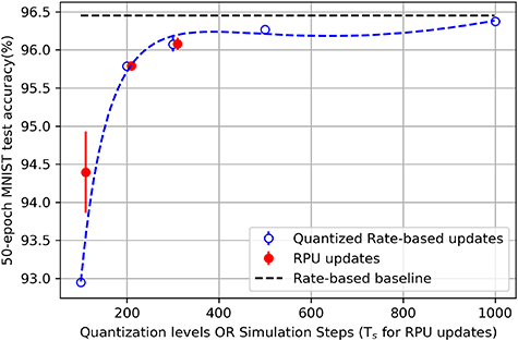
As shown in figures 4(b) and (c), there is a big discrepancy in the precision of the weight updates computed by the rate-based method and the temporally local method. In view of this knowledge, we train an SNN with temporally local weight updates across a range of simulation steps, ($T_s \in \{100, 200, 300\}$) and with appropriately quantized baseline rate-based updates ($T_s = 50$) using $30\,000$ training samples of the MNIST dataset for 50 epochs. We find in our experiments, as shown in figures 6 and 7, that simply quantizing the rate-based weight updates with the appropriate number of levels can provide a reliable prediction of the learning performance of the proposed RPU-inspired temporally local weight updates for varying simulation steps (T_s ). Furthermore, we find that the performances of the quantized rate-based weight updates and temporally local weight updates converge with increasing T_s and increasing number of training epochs. In figure 7, we extrapolate to find that $T_s = 1000$ would be sufficient for the temporally local weight updates to match the performance of the baseline rate-based weight updates. In figure 8, we extend the training of the SNN with quantized rate-based weight update simulations, both in terms of training data ($50\,000$ training samples) and epochs (200 epochs) and find that the performance difference seen in the shorter and smaller training (50 epochs) for low number of simulation steps, i.e. $T_s = 300$ (figures 6 and 7) could disappear (become same as $T_s = 1000$) in the long run (200 epochs). After establishing this equivalence, we can now continue to use rate-based update simulations to efficiently predict the performance of the RPU-inspired updates for a large variety of datasets.

Zoom In Zoom Out Reset image size

Zoom In Zoom Out Reset image size

Zoom In Zoom Out Reset image size

3.3.1. MNIST

3.3.2. Generalization to FMNIST, EMNIST

3.3.3. Naturally spiking input dataset—Neuromorphic-MNIST

Neuromorphic-MNIST [35] is a neuromorphic dataset where MNIST images are recorded by an address event representation (AER) sensor programmed with fixed motions to generate spiking representations of the images. For our simulations, we use the standard ToFrame preprocessing of the Tonic Python library [36] to convert the raw AER data of the N-MNIST samples into usable spike-trains. For any given N-MNIST AER spike, the preprocessing code first performs basic outlier detection by considering the number of spikes issued by neighboring neurons within a fixed time window and if it crosses a threshold, then the microsecond-level AER spike is extended into a millisecond-level frame pixel. This software-level preprocessing is functionally equivalent to pulse extender circuits, such as the ones described in [37] that are normally used to interface with AER sensors. Through this process, the approximately 300 ms ($300\,000\,\mu$s) long N-MNIST AER samples are converted into clocked N-MNIST samples, each containing approximately 300 frames of spikes for further processing. This is also unavoidable for practical simulations as it is both infeasible to perform SNN simulations with 300 000 timesteps (as would be necessary to maintain the AER timing precision) as well as unnecessary as the raw AER data is very sparse.

Since there is a temporal aspect to the data in N-MNIST, we use a fixed and randomly connected spiking reservoir [38, 39] to perform a basic level of temporal processing before the resultant spike rates of the reservoir neurons are encoded by Poisson random spike-trains and input to a two-layer SNN that is trained for the classification task by our algorithm as shown in figure 9.

Zoom In Zoom Out Reset image size

In our algorithm, the spiking rates of the reservoir neurons are recoded as Poisson spike trains. Recoding of the original reservoir neuron spike-trains into rate-based Poisson spike-trains needs to be done during the training phase to ensure that we generate stochastic spike-train inputs for the learning algorithm. For inference, we can directly use the reservoir spike trains as input without having to recode them as Poisson spike trains.

In our simulations, we have computed the spike rate calculation after the reservoir layer in two different ways:

Ideal computation: By counting the total number of spikes issued by each reservoir neuron and normalizing it by the number of simulation steps used for the Reservoir simulation ($\sum_t s_x^\mathrm{Reservoir}(t)/T_s$).

Realistic computation: By convolving the reservoir spike-trains with an exponential kernel and using a leaky integrator to estimate the instantaneous spike-rate—which is used to generate the random Poisson spike trains

The second method of recoding reservoir neuron spike rates into Poisson spike trains outlined above would not require much overhead. It can be accomplished simply by using an additional layer of synapses (to implement the convolution with an exponential kernel) connecting each reservoir neuron to a stochastic spiking neuron, [40] as shown in figure 10.

Zoom In Zoom Out Reset image size

Table 4 contains the comparisons of the performance of our method with the state-of-the-art in SNN learning. The equations and parameters for the Reservoir simulation are replicated from the basic 1000-neuron Reservoir Model described in [41].

Table 4. Generalization of SSNN-BP to N-MNIST dataset.

Model	Network	Loss and Regularizer	N-MNIST test-set accuracy (%)
HM2-BP [14]	2 layer H1 = 800	MSE	98.84
DECOLLE [42]	Convolutional neural network with 3 (7 × 7) Conv-Pool layers followed by a fully connected layer	MSE and dropout	99 * (Results on a subset of the data with 20 000 training samples and 1000 test samples)
This work	1000-neuron reservoir + 2 layer SNN, H1 = 1280	softmax-CE and dropout for 2-layer SNN only	98.26 +/- 0.02

The supervised training of neural networks using BP of errors is a data-intensive task. There has been a significant thrust to transfer these operations in/near-memory and on-chip for latency and power efficient forward and backward propagation [43]. Large neuromorphic cores of thousands of fast communicating neurons and energy efficient address event representation between hundreds of such cores have been demonstrated in digital and analog mixed mode hybrid design in hardware [44]. Chips like Neurogrid [43], TrueNorth [2], SpiNNaker [45], and Loihi [3] have made the realization of very large-scale neural networks possible, bringing down the time and energy complexity of network dynamics by several orders (3–4) of magnitude compared to conventional Processor and GPU simulations [44, 46].

The present trend in the neuromorphic very large scale integration (VLSI) is to increase in scale while maintaining the simplicity of individual units. Most implementations make use of simple leaky, IF neurons with methods to stochastically generate and propagate information only using spikes. These implementations also offer simple learning rules based on spike timings (STDP). The hardware acceleration benefits are not limited to just forward and backward propagation. Weight gradient calculation and weight update is another field where the role of hardware-enabled efficiency is extremely critical. As described earlier, the proposal of RPU enables simultaneous calculation of gradients and write-back in large crossbar arrays of analog memories holding network weights. Since RPUs depend on the generation of stochastic and pulsed representation of activations and errors, they are naturally well-suited for SNNs: spikes easily replace the stochastic pulses needed for weight update calculation to achieve the same effect when combined with spike coincidence-based learning rules.

However, due to the nature of RPU-based stochastic multiplication, this type of training algorithm is mainly relevant for clocked spiking systems where voltage pulses can align in time for predictable periods of time (i.e. a clock cycle). This is the case because we are using an RPU-based approach which requires pulse co-incidence to update the weights and is a common assumption for RPU-capable memories proposed as synapses, including analog memories [23, 31, 47–49]. As such, pulse-extender circuits, such as ones described in works such as [37, 50, 51] would be required to interface data from asynchronous AER sensors with our RPU-based SNN learning system

Several device-level implementations of stochastic neurons using resistive memories like phase change memories [52], bulk switching Pr_1-xCa_xMnO₃ resistive random access memory (PCMO RRAMs) [53] and nanomagnets [54] have been proposed. Similarly, analog memories for synapses like charge trap flash [23] and dynamic random acess memory (DRAM)-like capacitors [47] with analog charge storage have shown the feasibility of RPU. Thus algorithms tailored to a generic description of an SNN and all computations done in spikes are readily transferable and scalable on neuromorphic hardware.