Abstract
Spike encoding of sound consists in converting a sound waveform into spikes. It is of interest in many domains, including the development of audio-based spiking neural network applications, where it is the first and a crucial stage of processing. Many spike encoding techniques exist, but there is no systematic approach to quantitatively evaluate their performance. This work proposes the use of three efficiency metrics based on information theory to solve this problem. The first, coding efficiency, measures the fraction of information that the spikes encode on the amplitude of the input signal. The second, computational efficiency, measures the information encoded subject to abstract computational costs imposed on the algorithmic operations of the spike encoding technique. The third, energy efficiency, measures the actual energy expended in the implementation of a spike encoding task. These three efficiency metrics are used to evaluate the performance of four spike encoding techniques for sound on the encoding of a cochleagram representation of speech data. The spike encoding techniques are: Independent Spike Coding, Send-on-Delta coding, Ben's Spiker Algorithm, and Leaky Integrate-and-Fire (LIF) coding. The results show that LIF coding has the overall best performance in terms of coding, computational, and energy efficiency.
Export citation and abstract BibTeX RIS

Original content from this work may be used under the terms of the Creative Commons Attribution 4.0 license. Any further distribution of this work must maintain attribution to the author(s) and the title of the work, journal citation and DOI.
1. Introduction
The problem of converting sound into spikes is of interest mainly in three application areas. First, it is relevant in computational models of the peripheral auditory system that aim to reproduce properties of audition [23]. Second, it is used in the silicon cochlea, a neuromorphic event-based microphone [18, 19] that outputs asynchronous spikes from an analog sound. Third, it is fundamental in the processing of audio through spiking neural networks (SNNs) which use spike representations as input.
In all of these areas, it is imperative to select the best spike encoding technique, i.e. the one that encodes the maximum amount of information from the original data [37]. A multitude of techniques can be used to convert signals to spikes, and there are two quantitative approaches to evaluate their efficiency against one another [29, 30]. These two approaches are decoding (e.g. [6, 10, 28, 42, 44]) and information theory (e.g. [7, 10]).
Evaluating spike encoding techniques with the decoding approach refers to either classification or stimulus reconstruction, which both consist in recovering (i.e. decoding) some piece of information about the original stimulus from the spikes. For example, speech classification is used in [42] to compare three auditory SNN front-ends, and in [44] and [10] to evaluate multiple spike encoding techniques. Stimulus reconstruction, on the other hand, is used for example in [28] and [6] to compare several spike encoding techniques.
The decoding approach has important drawbacks that limit the quantitative evaluation of spike encoding techniques, notably the information loss due to the further processing of spikes and the influence of the choice of decoding models on the results.
The most important limitation of the decoding approach is the information loss due to further processing of spikes (e.g. processing with a SNN). The data processing inequality, a fundamental result in information theory, says that one can never gain information with further processing of data, only potentially lose it [4]. Thus, if one were to use decoding to compare different spike encoding techniques, one would not be leveraging the total information available in the spikes but only a fraction of this total information, because the additional processing on the spikes inherent in the decoding approach destroys some information [29, 30]. The information left is only a lower bound on the total information that the spike trains carry.
Moreover, when performing decoding, one can never be assured of having the theoretically best classifier or stimulus decoder, only a lower bound on it. Because using different decoding models leads to different results, the performance measured in decoding is not independent of the choice of the models introduced [25, 30].
In view of the limitations of the decoding approach, information theory offers more rigorous and direct quantitative metrics of performance [2]. In contrast to decoding, information theory measures the total information captured by the spikes without introducing models or additional processing that can cause information loss. Information theory has been used for example in [7] and [10] to evaluate spike encoding techniques.
This work proposes three rigorous metrics of efficiency based on information theory, and uses them to compare the performance of different spike encoding techniques for audio applications 1 . The first metric, coding efficiency, measures the fraction of information that the spikes capture from the total information present in the signal to be encoded. The second, computational efficiency, measures the information encoded subject to abstract costs imposed on the algorithmic operations of the spike encoding techniques in an implementation-independent way. The third, energy efficiency, measures the actual energy expended in the spike encoding task in an implementation-dependent way.
In the rest of the article, the proposed efficiency metrics are presented in detail, and they are used to quantitatively evaluate the performance of four spike encoding techniques on the encoding of a cochleagram representation of speech data. The four spike encoding techniques are: Independent Spike Coding (ISC), Send-on-Delta (SoD) coding, Ben's Spiker Algorithm (BSA), and Leaky Integrate-and-Fire (LIF) coding. The results show that LIF coding has the overall best performance. The potential relationship between the efficiency metrics and application performance is further illustrated with a classification example.
2. Spike density, mutual information and efficiency metrics
The efficiency metrics proposed in this work are based on the mutual information between the signal to be encoded and the spikes. In this section, spike density is defined, the methodology to estimate the mutual information is presented, as well as the three proposed efficiency metrics.
2.1. Spike density
A dynamic signal ![$x[n]$](https://content.cld.iop.org/journals/2634-4386/3/2/024007/revision2/nceacd952ieqn1.gif) is encoded into a spike train
is encoded into a spike train ![$w[n]$](https://content.cld.iop.org/journals/2634-4386/3/2/024007/revision2/nceacd952ieqn2.gif) by a given spike encoding technique
2
. Every spike encoding technique has parameters that modulate the number of spikes produced in the spike train. These parameters can be configured to yield spike trains of varying density, ranging from very sparse (few spikes) to very dense (many spikes).
by a given spike encoding technique
2
. Every spike encoding technique has parameters that modulate the number of spikes produced in the spike train. These parameters can be configured to yield spike trains of varying density, ranging from very sparse (few spikes) to very dense (many spikes).
In this work, a spike train ![$w[n]$](https://content.cld.iop.org/journals/2634-4386/3/2/024007/revision2/nceacd952ieqn3.gif) is taken to be a discrete binary time signal (figure 1) with ones representing spikes. Different encoding parameter configurations can lead to spike trains of different firing rates. The maximum attainable firing rate is when there are spikes at every time step. In such a case, the firing rate is equal to the sampling rate of the input signal. Spike density ρ is defined as the normalized mean firing rate,
is taken to be a discrete binary time signal (figure 1) with ones representing spikes. Different encoding parameter configurations can lead to spike trains of different firing rates. The maximum attainable firing rate is when there are spikes at every time step. In such a case, the firing rate is equal to the sampling rate of the input signal. Spike density ρ is defined as the normalized mean firing rate,

where N is the total number of samples in the spike train ![$w[n]$](https://content.cld.iop.org/journals/2634-4386/3/2/024007/revision2/nceacd952ieqn4.gif) , and the absolute value accounts for the case of spike encoding techniques which yield bipolar spike trains (where spikes can be positive or negative, such as for example SoD coding). Spike density is comprised between 0 (representing the extreme case of no spikes at all) and 1 (representing the extreme case of a spike at every sample).
, and the absolute value accounts for the case of spike encoding techniques which yield bipolar spike trains (where spikes can be positive or negative, such as for example SoD coding). Spike density is comprised between 0 (representing the extreme case of no spikes at all) and 1 (representing the extreme case of a spike at every sample).
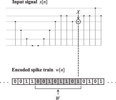
Figure 1. The discrete random variable X associated with the input signal is the discretized instantaneous amplitude of the input signal ![$x[n]$](https://content.cld.iop.org/journals/2634-4386/3/2/024007/revision2/nceacd952ieqn5.gif) . The discrete random variable W associated with the spike train is the vector of samples in a sliding overlapping window of observation of fixed length. The mutual information between X and W is the information that the spike vectors encode on the signal's amplitude. The spike train shown in the figure is just an illustration.
. The discrete random variable W associated with the spike train is the vector of samples in a sliding overlapping window of observation of fixed length. The mutual information between X and W is the information that the spike vectors encode on the signal's amplitude. The spike train shown in the figure is just an illustration.
Download figure:
Standard image High-resolution imageBy varying the parameters of the spike encoding techniques that modulate the spike density and evaluating the information content of spike trains at different densities, a complete picture of the performance of a spike encoding technique can be established. Moreover, spike density offers a common scale to compare the performance of different spike encoding techniques which have different parameters.
2.2. Mutual information estimation
2.2.1. Discrete random variables
The mutual information is estimated between two discrete random variables, one representing the signal, and the other representing the spikes. The goal is to estimate how much information the spike train captures on the amplitude of the signal to be encoded. The variables of interest are therefore, respectively, the dynamic signal's amplitude and temporal patterns of spikes.
The mutual information is taken between discrete random variables. The dynamic signal is, however, continuous in amplitude. Therefore, it has to be discretized in amplitude. In this work, k-means clustering [12] is used to quantize the signal's amplitude to 256 levels. This yields a non uniform scalar quantization of the amplitude distribution. The discrete random variable X associated with the signal is then built from the discretized amplitude of the signal.
Since a spike train is binary, it cannot encode all these amplitude levels in a single sample. It is therefore necessary to look at patterns of spikes in a window of observation in the spike train in order to recover information on the signal's amplitude. The discrete random variable W associated with the spike train is built from vectors of samples in sliding overlapping windows of observation of fixed length (figure 1). A window length of eight samples is used in this work.
2.2.2. Mutual information
The mutual information  between the signal and the spikes is estimated in bits:

where  is the joint probability between X and W, and P(x) and P(w) are the marginal probabilities [4].
2.2.3. Encoding latency
Spike encoding techniques can introduce a latency where the spike train at a certain instant in time is maximally informative on the amplitude of the signal at a past time instant. This has to be taken into account when estimating the mutual information. This latency is corrected for by successively shifting the spike train in the past by one sample at a time and evaluating the mutual information at every time shift. The 'true' mutual information is taken for the time shift for which it is maximal. If no latency is present, this corresponds to the case with no time shift.
2.2.4. Sampling bias
In practice, mutual information estimation suffers from a systematic error referred to as 'bias'. This bias is due to the inevitable finite sampling of data and it has been extensively studied in the literature [26]. This means that a naive estimation of mutual information using (2) would give biased results.
To correct this bias, the standard quadratic extrapolation method is used [26, 36, 38]. In this method, the mutual information is estimated using multiple fractions of the data (half, quarter, etc), and using these estimations to quadratically extrapolate to the case of infinite data which is taken to be the 'true' value of the mutual information. The corrections in the extrapolation are small.
2.3. Efficiency metrics
This subsection presents the three proposed efficiency metrics. The first metric, coding efficiency, estimates the fraction of information encoded in the spikes from the total information available in the signal to be encoded. The other two efficiency metrics take into account the cost of the spike encoding techniques, which characterizes the trade-off between encoding the maximum information and consuming the least energy. Computational efficiency attributes abstract costs to the algorithmic operations of the spike encoding techniques, whereas energy efficiency estimates the empirical energy expenditure specific to the data and implementation of the spike encoding techniques.
2.3.1. Coding efficiency
The maximum achievable mutual information is determined by the statistical structure of the signal's random variable X and is given by the entropy

which is the total amplitude information present in the signal to be encoded. If W completely characterizes X, then the mutual information is equal to H(X), which means that the encoding is perfect. The coding efficiency ε is defined as the fraction of information that is encoded in the spikes:

2.3.2. Computational efficiency
Every spike encoding technique has algorithmic operations that incur costs at every timestep. The cost can be decomposed into fixed and variable costs, respectively Cf and Cv . The fixed cost Cf is incurred whether or not a spike is produced at the timestep, and represents all the algorithmic operations that are needed to update the variables. The variable cost Cv , however, is only incurred when a spike is produced, and involves the operation of spike production, as well as any other algorithmic operations required after a spike is produced [14, 17, 35].
The computational cost of the algorithmic operations of spike encoding techniques is characterized using the abstract unit 'op' (corresponding to operations). This permits the abstract decomposition of the cost into fixed and variable computational costs in an implementation-independent way, based solely on the pseudo-code of the spike encoding technique.
For a given spike encoding technique, the average computational cost rate  (in op/timestep) only depends on the spike density ρ (which can be seen as the average number of spikes produced per timestep),

with the fixed cost Cf and the variable cost Cv estimated in op/timestep from the pseudo-code of the spike encoding techniques.
The computational efficiency ηC , measured in bit/op, is then

2.3.3. Energy efficiency
Energy efficiency is based on the direct estimation of the energy cost rate  of the spike encoding on the specific data used and the specific implementation of the spike encoding techniques. This energy cost rate depends on the spike density.
In this work, the energy cost rate  is estimated using the pyJoules Python library [33], which monitors the energy consumed by CPUs using Intel's Running Average Power Limit technology. This approach gives an empirical measurement of the energy consumed, but it is dependent on the specific input data, the implementation of the spike encoding techniques, and the processor architecture used.
The energy efficiency ηE , measured in bit/nJ, is then

3. Data and spike encoding
The proposed efficiency metrics are used to quantitatively evaluate the performance of four spike encoding techniques in an audio setting. This section details the data used (the speech stimulus and its cochleagram representation), as well as the four spike encoding techniques that are evaluated.
3.1. Stimulus and cochleagram
The speech stimulus used is an audio sequence of 20 min made by concatenating spoken digits from the TIDIGITS adult dataset [11] chosen at random and sampled at 20 kHz.
The input speech stimulus is transformed into a cochleagram, which gives an approximation of auditory nerve fiber spiking probabilities. To compute the cochleagram (figure 2), the signal is first passed through an infinite impulse response Gammatone filterbank with eight channels. The filerbank has center frequencies distributed on the equivalent rectangular bandwidth scale spanning the range from 100 Hz to 8 kHz. It approximates the vibrations of the basilar membrane [23, 27]. Inner hair cells are then modeled with half-wave rectification followed by cubic-root compression and low-pass filtering at 10 Hz. This low-pass filtering allows to extract the envelope of the oscillations. Finally, the signal is decimated to 1 kHz and normalized to form the cochleagram. The brian2hears Python library [9] is used for the cochleagram extraction.

Figure 2. Block diagram of the cochleagram extraction. The speech stimulus is first passed through a bank of eight IIR Gammatone filters. The output of the filters is half-wave rectified, cubic-root compressed, and low-pass filtered at 10 Hz to model the effects of inner hair cells and extract the envelope of the oscillations. The output is then decimated to 1 kHz. The cochleagram is normalized overall to a maximum of 1.
Download figure:
Standard image High-resolution image3.2. Spike encoding
Four spike encoding techniques are evaluated: ISC, SoD coding, BSA, and LIF coding. They take as input a dynamic signal (i.e. the output ![$x[n]$](https://content.cld.iop.org/journals/2634-4386/3/2/024007/revision2/nceacd952ieqn11.gif) of a given cochleagram channel). Thus, each of the cochleagram's channels is encoded separately and independently into a single spike train. The pseudo-code for each of these techniques is provided in the
of a given cochleagram channel). Thus, each of the cochleagram's channels is encoded separately and independently into a single spike train. The pseudo-code for each of these techniques is provided in the
3.2.1. Independent Spike Coding (ISC)
In ISC, the instantaneous firing probability in a cochleagram channel is used to emit spikes stochastically and independently, resulting in a non homogeneous Poisson process. Specifically, the probability of a spike at sample n is

where a is a scaling factor that modulates the density of the resulting spike train.
ISC is used in [34] to encode cochleagrams for speech recognition. It is also the standard approach to generate spikes in computational models of the peripheral auditory system, such as those of Carney [3] and Meddis [22]. The Meddis model is used in [5] to produce the Heidelberg audio spike datasets for SNNs.
3.2.2. SoD coding
In SoD [24], a spike is emitted when the net change in the signal's amplitude is at least equal to a fixed value (Δ), with the spike being an ON event if the change is positive, and an OFF event if the change is negative. This makes it possible to have a reconstruction of the original signal from the spikes, since between any two consecutive spikes, the signal has changed by  . Specifically, the first and the kth spikes are emitted at samples:


Bipolar spikes (+1 and −1) are used, although it is equivalent to use two different unipolar spike trains. The threshold Δ modulates the density of the spike train.
SoD is used in [47] for speech recognition, and in the silicon cochlea model in [43]. SoD is discussed in other works under the name 'step-forward encoding' [28].
3.2.3. Ben's Spiker Algorithm (BSA)
BSA [32] is based on the reverse convolution of the signal with a FIR filter h of length M. It emits spikes based on a simple heuristic comparing the filter's impulse response with the signal, such that the convolution of the resulting spike train with the filter gives a reconstruction of the original signal. At each instant, two error metrics are computed:


If  , with θ a threshold, a spike is emitted and the filter is subtracted from the signal. BSA requires input signals to be comprised between 0 and 1, as the maximum signal value that can be reconstructed is equal to the sum of the filter's coefficients. BSA's threshold parameter θ modulates the density of the spike train.
BSA is used in works by Schrauwen and colleagues [31, 40–42], Maass and colleagues [15, 16], and Li and colleagues [13, 46].
3.2.4. LIF coding
In this method, the signal is fed directly as a membrane current to be integrated by a neuron with discretized equation


where u is the neuron's membrane potential, τ its time constant, and the signal to be encoded ![$x[n]$](https://content.cld.iop.org/journals/2634-4386/3/2/024007/revision2/nceacd952ieqn14.gif) becomes the membrane current. The resistance in the model is assumed to be equal to 1. If the potential crosses a threshold θ, the neuron emits a spike, and its potential is reset to zero (resting potential). LIF coding's firing threshold θ modulates the density of the spike train.
becomes the membrane current. The resistance in the model is assumed to be equal to 1. If the potential crosses a threshold θ, the neuron emits a spike, and its potential is reset to zero (resting potential). LIF coding's firing threshold θ modulates the density of the spike train.
LIF coding is used for example in speech recognition in [1] and [45]. LIF coding is also used to transduce the inner hair cell signal into spikes in the silicon cochleae proposed in [20, 21, 39].
4. Results and discussion
This section presents the results of the quantitative evaluation of the four spike encoding techniques using the proposed efficiency metrics, as well as an application example that explores the relationship between the information-theoretical approach and application performance.
4.1. Coding efficiency
The coding efficiency  is estimated for each of the eight cochleagram channels, and the mean coding efficiency is shown in figure 3. At the boundaries of the spike density, where the spike trains are too sparse or too dense, not much information can be encoded, because there is not much variability in the spike trains. It is somewhere between the two extremes that the higher coding capacity offers room to maximally encode the signal. Therefore, mutual information curves have concave shapes relative to spike density. The results show that overall, ISC and SoD have low coding efficiency, while LIF and BSA have the highest coding efficiency (with BSA's coding efficiency being slightly higher than LIF's).

Figure 3. Coding efficiency as a function of spike density ρ for the four spike encoding techniques. The curves show the mean of the coding efficiency over the eight cochleagram channels, and the error bars show the standard deviation. For BSA, the results are shown for the overall best filter found (8 taps), and similarly for the membrane time constant of LIF coding (τ = 8 ms). ISC and SoD have low coding efficiency while BSA and LIF have the highest coding efficiency.
Download figure:
Standard image High-resolution imageThe stochastic nature of ISC introduces noise that degrades the spike train's information content, which can explain its low coding efficiency. SoD encodes the changes in a signal. Intuitively, this means that the spike train can only inform on changes in levels (relative amplitude), not on the absolute values of the levels (exact value of the amplitude). To recover information on the latter, one would need to know the initial level, and keep track of all the changes up to the present. For this reason, SoD might show good performance if it is rather the derivative of the amplitude that is the information of interest, and not the amplitude itself as is the case here. BSA has the highest mean coding efficiency of 34.6% (standard deviation 3.2%) for a spike train of 30.6% density, but it should be noted that the threshold parameter is traditionally chosen for the optimal reconstruction of the signal from the spikes, and the threshold that is optimal for that signal's reconstruction might be different from the threshold that is optimal in terms of information. Interestingly, LIF's mean coding efficiency closely follows that of BSA, but peaks at a slightly lower efficiency of 32.6% (standard deviation 2.3%) for a spike train of 40% density, thus a higher density than for BSA's maximum coding efficiency.
It should be noted that overall the best mean coding efficiency is only 34.6%, which shows that most of the amplitude information is discarded when encoding a signal into a single spike train even in the best case scenario.
4.2. Computational and energy efficiencies
Next, the spike encoding techniques are compared in terms of their computational and energy efficiencies. Only the results for BSA and LIF are included in this article, as the other two encoding techniques (ISC and SoD) have significantly much less coding efficiency.
For the computational efficiency, rather than trying to capture the precise costs of the operations of each of the two spike encoding techniques, the cost is characterized abstractly in terms of the algorithmic operations involved. Costs of operations are taken as a rough approximation. Addition, subtraction, comparison, and absolute value are all assumed to cost 1 op. Multiplications are assumed to cost 2 op since they are usually significantly more costly compared to the other operations [8]. For the energy efficiency, the actual energy consumed in spike encoding is estimated, with this estimation being specific to the implementation, data, and architecture used.
For LIF (see algorithm  (2 op) followed by addition of the input value (1 op). The membrane potential is then compared to the firing threshold (1 op). Thus, the fixed cost is
  op. The variable cost Cv
, incurred only when a spike is produced, involves producing the spike (1 op) and resetting the membrane potential to zero (1 op). Thus, the variable cost
op. The variable cost Cv
, incurred only when a spike is produced, involves producing the spike (1 op) and resetting the membrane potential to zero (1 op). Thus, the variable cost  op.
op.
For BSA (see algorithm  op. The variable cost, incurred only when a spike is produced, involves producing the spike (1 op) and updating the input by subtracting the filter's impulse response (M op). Thus, the variable cost is
  op.
op.
Figure 4 shows the computational cost rate  (figure 4(a)) and the energy cost rate
  (figure 4(a)), as well as the computational efficiency ηC
(figure 4(c)) and the energy efficiency ηE
(figure 4(d)) of both spike encoding techniques.
(figure 4(a)), as well as the computational efficiency ηC
(figure 4(c)) and the energy efficiency ηE
(figure 4(d)) of both spike encoding techniques.

Figure 4. (a) and (b): Computational cost rate  and energy cost rate
  as a function of the spike density ρ for BSA and LIF (in log y-axis). For the energy cost rate (b), the curves show the mean estimated cost rate over the eight cochleagram channels, and the error bars show the standard deviation. As can be observed, BSA is much more costly than LIF. (c) and (d): Computational efficiency ηC
and energy efficiency ηE
as a function of the spike density ρ for BSA and LIF (in log y-axis). The curves show the mean computational efficiency over the eight cochleagram channels, and the error bars show the standard deviation. LIF has much higher computational and energy efficiencies than BSA as a consequence of being a less costly spike encoding technique. The results of the computational approach are very similar to those of the energy approach. The parameter values used for BSA and LIF are the same as for those shown in figure 3.
as a function of the spike density ρ for BSA and LIF (in log y-axis). For the energy cost rate (b), the curves show the mean estimated cost rate over the eight cochleagram channels, and the error bars show the standard deviation. As can be observed, BSA is much more costly than LIF. (c) and (d): Computational efficiency ηC
and energy efficiency ηE
as a function of the spike density ρ for BSA and LIF (in log y-axis). The curves show the mean computational efficiency over the eight cochleagram channels, and the error bars show the standard deviation. LIF has much higher computational and energy efficiencies than BSA as a consequence of being a less costly spike encoding technique. The results of the computational approach are very similar to those of the energy approach. The parameter values used for BSA and LIF are the same as for those shown in figure 3.
Download figure:
Standard image High-resolution imageAs can be observed from figures 4(a) and (b), it is clear that BSA is more computationally costly than LIF. In fact, this characterization of computational costs (an implementation-independent approximation) arrives at very similar results when compared to the measurement of the actual energy cost rate using the pyJoules Python library (actual energy consumed in the specific implementation with an Intel® Xeon® Processor E5-2683 v4 architecture).
As can be observed from figures 4(c) and (d), both BSA and LIF have peak computational and energy efficiencies in the spike train density range between 25% and 35%. Unsurprisingly, LIF's computational efficiency is much higher than BSA, which makes it a more computationally and energetically efficient spike encoding technique than BSA.
4.3. Information theory and application performance
The potential relationship between information-theoretic spike encoding evaluation and application performance is explored in this section on the example of isolated spoken digit recognition. The same TIDIGITS dataset is used. It has a total of 11 classes: 'zero' through 'nine', plus 'oh'. The training and test partitions have 2464 and 2486 audio examples, respectively. The cochleagram representation of the spoken digits is encoded into spikes using LIF coding, and the firing threshold is considered as the parameter to optimize.
First, the search complexity is discussed and compared between the decoding and the information-theoretic approaches. The former approach consists in choosing the encoding parameters that optimize classification accuracy as the performance metric, while the latter approach consists in choosing the parameters that optimize an information-theoretic efficiency metric instead. In this discussion, the optimization is performed with a grid search, i.e. an exhaustive search through a manually specified set of parameter values. The discussion on search complexity is followed by a comparison between the two approaches when performing a classification task using three different classifiers.
4.3.1. Search complexity
The signals in the different cochleagram channels have different properties, and each channel has to be encoded into a spike train. This means that the firing threshold should be specifically tuned for each channel.
In the decoding approach, a grid search has to be run on the firing thresholds to find the values that maximize the performance metric, taken here as the classification accuracy. This grid search cannot be carried out independently on each cochleagram channel. In fact, the firing threshold for each channel has to be optimized together with the threshold for the other channels when performing the classification task. The possible combinations of parameter values leads to a combinatorial explosion that makes this approach intractable. For example, suppose that a grid search is run on 10 values of the firing threshold. The classification task therefore has to be run a total of 108 (one hundred million) times to explore the grid search fully. This number represents all the possible combinations of parameter values across the eight cochleagram channels, and it scales exponentially with the number of channels.
In the information-theoretic approach, the metric to optimize is an efficiency metric such as the ones proposed in this work, rather than classification accuracy. These efficiency metrics are estimated for each channel independently of the others, and therefore the search complexity in this case is tractable. In fact, with 8 cochleagram channels and 10 parameter values in the grid search for example, there is a total of only  computations of the chosen efficiency metric to explore the grid search fully. This number scales linearly with the number of channels, as opposed to the exponential relationship seen before.
4.3.2. Classification results
The decoding and the information theoretic approaches are compared here on a classification task.
In the information-theoretic approach, energy efficiency (mutual information over energy rate) is taken as the metric to optimize. The LIF firing threshold in each channel is chosen as the value in the grid search that maximizes the energy efficiency in that channel. Note that in this case, the firing threshold can be different from channel to channel.
In the decoding approach, since it is not feasible to carry out the entire grid search in a tractable manner, a simplification is made: the LIF firing threshold is constrained to be the same for all channels. The results obtained with this simplification represent a lower bound on the best performance that could be obtained with a full grid search.
For a given spoken digit from the dataset, the spikes in each spike train are counted and averaged in 25 bins. The bins have 50% overlap. Since the audio files of the spoken digits are variable in duration, the bin width for each spoken digit is also variable. There is a total of 200 features per spoken digit (25 bins × 8 spike train channels). Three classifiers are used from the scikit-learn Python library: support vector machine with a radial basis kernel function, k-nearest neighbors with the Euclidian distance as a metric and k = 5 neighbors, and random forest with 100 estimators.
Classification results are shown in figure 5. In all graphs, classification accuracy for the decoding approach grid search (solid line) plateaus in the range approximately comprised between 5% and 40% spike density. In the information-theoretic approach, the grid search is carried out using the energy efficiency as performance metric, and the firing thresholds are chosen as the ones that maximize that metric in each channel. The classification task is then run with this single parameter configuration (red cross markers). The spike trains found have an average density of 32% and achieve a classification accuracy that is only slightly lower than the best accuracies found with the decoding approach. As can be observed in figure 5, the grid search of the decoding approach finds slightly better classification accuracies that can be achieved with lower spike densities.

Figure 5. Classification accuracy on the spike-encoded TIDIGITS isolated digit recognition application for three classifiers. The blue solid lines show the classification accuracy obtained with the decoding approach grid search over the LIF firing threshold (with the thresholds constrained to be the same for all cochleagram channels). The classification accuracy plateaus in this approach in the range approximately comprised between 5% and 40% spike density. The red cross markers show the classification accuracy achieved with the information-theoretic approach, with energy efficiency as the optimization metric. This accuracy is comparable to the best accuracy obtained with the decoding approach for each classifier.
Download figure:
Standard image High-resolution image
These results show that although the information-theoretic approach does not guarantee the best performance, it can be used to find an initial parameter configuration that gives a decent performance. This can be used in turn as a baseline in further parameter tuning with the aim of achieving better performance or lower spike density or both. Additional parameter tuning can be efficiently carried out for example with evolutionary optimization techniques.
It is also relevant to note that the shape of the curves in figure 5 is similar to those of the information-theoretic efficiency metrics proposed in this work (figures 3 and 4). Nevertheless, a direct comparison is not possible because the firing threshold has been constrained to be the same for all cochleagram channels in figure 5.
4.4. Summary
There are many techniques that can be used in the spike encoding of sound. These techniques have been evaluated using two approaches: decoding and information theory. In the decoding approach, performance is evaluated in applications that use models and further process the spike trains destructively, causing information loss. In the information-theoretic approach, the total information captured by the spikes is measured without introducing models or additional processing on the spikes.
In this work, the performance of four spike encoding techniques is quantitatively evaluated based on three proposed information-theoretic efficiency metrics
- (i)Coding efficiency measures how much information is encoded in the spikes from the total information available in the signal.
- (ii)Computational efficiency incorporates the cost of spike encoding by attributing abstract costs to the algorithmic operations of the spike encoding techniques (implementation-independent).
- (iii)Energy efficiency incorporates the cost of spike encoding by empirically estimating the energy expended in the operation of spike encoding techniques (implementation-dependent).
These metrics allow to assess the overall performance of the spike encoding techniques:
- Independent Spike Coding, which is the standard method in computational auditory modeling, is shown to have poor coding efficiency, which is not surprising: the stochastic nature of ISC's spike generation introduces noise in the spike trains that degrades the information content.
- Send-on-Delta coding, which is an event-based sampling scheme that is popular in neuromorphic sensors, is shown to have poor coding efficiency as well, as it is unable to effectively encode the amplitude information: SoD only codes relative changes in amplitude, not absolute values.
- Ben's Spiker Algorithm, which is based on stimulus estimation, is found to have the highest coding efficiency out of the four techniques, but it is computationally complex and thus suffers in terms of computational and energy efficiencies.
- Leaky Integrate-and-Fire coding has slightly less coding efficiency than BSA, but has much higher computational and energy efficiencies because it is a less costly spike encoding technique. Overall, LIF coding shows the best performance out of the four spike encoding techniques considered in this work.
Furthermore, as shown on the example of isolated spoken digit recognition presented here, using the information-theoretic efficiency metrics to optimize spike encoding parameters is tractable and leads to an initial baseline solution that shows decent application performance. This baseline solution can then be used in more efficient parameter tuning to try to improve performance or lower spike density or both.
5. Conclusion
In this work, efficiency metrics based on information theory are proposed and used to evaluate the performance of spike encoding techniques for audio. The metrics are: coding efficiency, computational efficiency, and energy efficiency. The quantitative evaluation based on these metrics shows that among four spike encoding techniques studied, LIF coding has the best overall performance in the encoding of cochleagram representations of speech data, and it is thus the preferred spike encoding technique for this type of data.
These important results are useful in guiding researchers in the selection of spike encoding techniques for their spike-based processing systems, and, more generally, in making spiking versions of audio datasets that are independent of applications.
Acknowledgments
This work was supported by the Fonds de Recherche du Québec—Nature et Technologie (FRQNT) and the Natural Sciences and Engineering Research Council of Canada (NSERC). We thank Luca Herranz–Celotti, Ismael Balafrej, and Sidi Yaya Arnaud Yarga for useful discussions. We also thank the reviewers for helpful comments.
Data availability statement
No new data were created or analysed in this study.
Appendix: Pseudo-code for spike encoding techniques
Algorithms 1 through 4 give the pseudo-code for the four spike encoding techniques evaluated in this work. Each algorithm's input is a signal to be encoded (i.e. a cochleagram channel signal ![$x[n]$](https://content.cld.iop.org/journals/2634-4386/3/2/024007/revision2/nceacd952ieqn25.gif) ) and a parameter configuration. The output is the encoded spike train
) and a parameter configuration. The output is the encoded spike train ![$w[n]$](https://content.cld.iop.org/journals/2634-4386/3/2/024007/revision2/nceacd952ieqn26.gif) .
.
| Algorithm 1. Independent Spike Coding (ISC) (section 3.2.1). |
|---|
| Input: signal x, scaling factor a |
| Output: spike train w |
1: 
|
2: for
 do
do
|
3: if
![$\mathrm{rand}\_\mathrm{uniform}(0,1) \lt x[n] \times a$](https://content.cld.iop.org/journals/2634-4386/3/2/024007/revision2/nceacd952ieqn29.gif) then
then
|
4: ![$w[n] \leftarrow 1$](https://content.cld.iop.org/journals/2634-4386/3/2/024007/revision2/nceacd952ieqn30.gif)
|
| 5: end if |
| 6: end for |
| 7: return w |
| Algorithm 2. Send-on-Delta (SoD) (section 3.2.2). |
|---|
| Input: signal x, delta Δ |
| Output: bipolar spike train w |
1: 
|
2: ![$b \leftarrow x[1]$](https://content.cld.iop.org/journals/2634-4386/3/2/024007/revision2/nceacd952ieqn32.gif)
|
3: for
 do
do
|
4: ![$d \leftarrow x[n] - b$](https://content.cld.iop.org/journals/2634-4386/3/2/024007/revision2/nceacd952ieqn34.gif)
|
5: if
 then
then
|
6: ![$w[n] \leftarrow 1$](https://content.cld.iop.org/journals/2634-4386/3/2/024007/revision2/nceacd952ieqn36.gif)
|
7: 
|
| 8: end if |
9: if
 then
then
|
10: ![$w[n] \leftarrow -1$](https://content.cld.iop.org/journals/2634-4386/3/2/024007/revision2/nceacd952ieqn39.gif)
|
11: 
|
| 12: end if |
| 13: end for |
| 14: return w |
| Algorithm 3. Ben's Spiker Algorithm (BSA) (section 3.2.3). |
|---|
| Input: signal x, filter h, threshold θ |
| Output: spike train w |
1: 
|
2: 
|
3: for
 do
do
|
4: 
|
5: 
|
6: for
 do
do
|
7: ![$e_1 \leftarrow e_1+|x[n-k]-h(M-k)|$](https://content.cld.iop.org/journals/2634-4386/3/2/024007/revision2/nceacd952ieqn47.gif)
|
8: ![$e_2 \leftarrow e_2+|x[n-k]|$](https://content.cld.iop.org/journals/2634-4386/3/2/024007/revision2/nceacd952ieqn48.gif)
|
| 9: end for |
10: if
 then
then
|
11: ![$w[n] \leftarrow 1$](https://content.cld.iop.org/journals/2634-4386/3/2/024007/revision2/nceacd952ieqn50.gif)
|
12: for
 do
do
|
13: ![$x[n-k] \leftarrow x[n-k] - h[M-k]$](https://content.cld.iop.org/journals/2634-4386/3/2/024007/revision2/nceacd952ieqn52.gif)
|
| 14: end for |
| 15: end if |
| 16: end for |
| 17: return w |
| Algorithm 4. Leaky Integrate-and-Fire (LIF) (section 3.2.4). |
|---|
| Input: signal x, time constant τ, threshold θ |
| Output: spike train w |
1: 
|
2: 
|
3: ![$u[1] \leftarrow x[1]$](https://content.cld.iop.org/journals/2634-4386/3/2/024007/revision2/nceacd952ieqn55.gif)
|
4: for
 do
do
|
5: ![$u[n+1] \leftarrow u[n] \, \mathrm{e}^{-\frac{1}{\tau}} + x[n]$](https://content.cld.iop.org/journals/2634-4386/3/2/024007/revision2/nceacd952ieqn57.gif)
|
6: if
![$u[n+1] \geqslant \theta$](https://content.cld.iop.org/journals/2634-4386/3/2/024007/revision2/nceacd952ieqn58.gif) then
then
|
7: ![$w[n] \leftarrow 1$](https://content.cld.iop.org/journals/2634-4386/3/2/024007/revision2/nceacd952ieqn59.gif)
|
8: ![$u[n+1] \leftarrow 0$](https://content.cld.iop.org/journals/2634-4386/3/2/024007/revision2/nceacd952ieqn60.gif)
|
| 9: end if |
| 10: end for |
| 11: return w |
Footnotes
- 1
An introductory work is available in [7].
- 2
Discrete-time signal processing notation is used where n is the integer sample index of the time-sampled signal x.