
Abstract
Cities are beginning to monitor atmospheric carbon dioxide (CO2) to assess the efficacy of their climate policies. However, changes in anthropogenic CO2 emissions must be separated from biospheric CO2 fluxes which have a large seasonal cycle. Urban vegetation (e.g. lawns, trees along street and in parks, etc) in developed land covers is often omitted in regional biogenic CO2 flux models. We set up a biosphere model to estimate the regional biogenic CO2 fluxes in New York City (NYC) and assess the importance of vegetation within developed land covers. The model incorporates a high-resolution (30 m) land cover map which identifies the mixture of impervious surfaces and vegetation that is ubiquitous across developed land covers. We designed three model scenarios to evaluate the role of developed land covers in regional biogenic CO2 fluxes by assuming (a) there is no vegetation versus scenarios where all remotely sensed vegetation in developed land covers is either (b) grassland or (c) deciduous forest. Despite relatively low tree canopy cover in NYC, the regional biogenic CO2 fluxes are surprisingly large when vegetation within the developed land covers is included. Furthermore, the types of vegetation within the developed land covers are crucially important for estimating regional biogenic CO2 fluxes, demonstrated by a doubling in estimates of total biogenic CO2 flux when this vegetation is assumed to be grassland compared to forest. Using a Lagrangian atmospheric transport model, we find that the regional biogenic CO2 uptake offsets up to 40% of atmospheric CO2 enhancements attributed to anthropogenic emissions in summer afternoons and completely balances on-road traffic in one of the most congested cities in the United States. Accurate characterization of the vegetation and biogenic carbon fluxes in cities are essential to the development of effective atmospheric monitoring tools. Future measurements should focus on constraining CO2 fluxes in urban grasslands (i.e. lawns).
Export citation and abstract BibTeX RIS

Original content from this work may be used under the terms of the Creative Commons Attribution 4.0 license. Any further distribution of this work must maintain attribution to the author(s) and the title of the work, journal citation and DOI.
1. Introduction
Urban areas contribute more than 70% of global anthropogenic carbon dioxide (CO2) emissions (IPCC 2014). Many cities have pledged to achieve net-zero carbon by 2050, but effective emission reduction can only be achieved if the sources are properly identified, quantified, and monitored (Davis et al 2017, Sówka and Bezyk 2018). Currently, two approaches are widely used to quantify CO2 fluxes—bottom-up inventories and models and top-down atmospheric inversions. The bottom-up methodology aggregates disparate local information and extrapolates to regional scales, while the top-down approach infers CO2 sources from variability in observed atmospheric CO2 concentrations. The two approaches are complementary with the top-down providing net fluxes for large representative regions and the bottom-up information about the underlying processes. The top-down approach is often used to evaluate bottom-up inventories.
Urban vegetation uptake of CO2 varies significantly on diurnal and seasonal time scales (Hutyra et al 2014, Hardiman et al 2017, Menzer and McFadden 2017, Miller et al 2020, Bezyk et al 2021). This variability in biogenic CO2 fluxes contributes to the fluctuations in CO2 concentrations observed in the urban atmosphere (e.g. 20% seasonality in Miller et al 2020) and is a significant source of uncertainty in accurately quantifying and tracking anthropogenic CO2 emissions (Sargent et al 2018, Park et al 2020). With a rapidly growing number of cities striving for both ambitious reductions in fossil fuel emissions and ambitious increases in tree canopy cover, the need for accurate assessments of biogenic CO2 is also rapidly increasing.
A commonly used bottom-up model for quantifying biogenic CO2 fluxes is the vegetation photosynthesis and respiration model (VPRM). VPRM is a light use efficiency model incorporating remote sensing and meteorological data and calculates two components of the biogenic CO2 fluxes—gross ecosystem exchanges (GEEs) and ecosystem respiration. The original VPRM has been modified to an Urban-VPRM version that accounts for the suppression of respiration rates by presence of impervious surface areas (ISAs) in urban areas (Hardiman et al 2017). VPRM has been applied at a range of spatial scales from 500 m (Hardiman et al 2017) to 1 km (Sargent et al 2018) to 2 km (Gourdji et al 2022) in urban areas. However, due to high spatial heterogeneity in land cover, higher-resolution ecosystem models with detailed representation of heterogeneous land covers are needed in urban areas for accurate modeling of CO2 fluxes and concentration variability. Feng et al (2016) and Sargent et al (2018) both suggest a 1 km resolution inventory better reproduces CO2 variability than 5 km and 10 km in Los Angeles and Boston, respectively. Hardiman et al (2017) suggest high-resolution (i.e. finer than 500 m) is needed to resolve CO2 sources and sinks in Boston. Miller et al (2018) use a 2 m spatial resolution land cover map to simulate GEEs in Minneapolis–Saint Paul metropolitan region and suggest high resolution imagery is necessary for revealing important spatial variability in GEE, but the contribution from respiration to the net carbon budget is not addressed. Accurate estimation of biogenic CO2 fluxes within urban areas needs higher resolution data.
A high-resolution (30 m) land cover map recently developed by Dewitz (2021) for the continental United States (US) makes the setup of a high-resolution Urban-VPRM possible. Dewitz (2021) introduces a unique land cover category—the mixture of impervious surface and vegetation within developed urban land covers, which are the most common land cover type in cities. Measurements of biogenic CO2 fluxes across developed land covers are relatively sparse (Miller et al 2018) and, to our knowledge, there are no observation-constrained parameters for this vegetation-ISA mixed land cover in VPRM, resulting in two major unknowns in modeling biogenic CO2 fluxes in an urban context. First, we do not know to what extent the vegetation in developed land covers contributes to the regional biogenic CO2 fluxes. Second, given that the vegetation across developed land covers is typically composed of different plant functional types (e.g. lawn vs. trees), it is unclear how sensitive model estimates of urban biogenic CO2 fluxes are to different vegetation types in these land covers.
The New York metropolitan area (NYMA) is the largest urban source of carbon in US (Gately and Hutyra 2018) and third largest globally (Moran et al 2018). New York City (NYC), the urban core of the NYMA, also has the most trees among US cities (estimated at 7 million, Treglia et al 2021) and there are hopes of planting another million trees to increase tree canopy cover from 20% to 30%. Like many cities, NYC also includes considerable amounts of lawn vegetation. Because of the varied vegetated land covers and large fossil fuel emissions, NYC presents a particularly important scientific opportunity to assess the importance of accurate characterizations of vegetation type/cover in quantifying the relative contributions of the biosphere and anthropogenic emissions to urban atmospheric CO2 concentrations.
The objectives of this study are (a) to demonstrate the applicability of the high-resolution Urban-VPRM in an urban context, initiating a modeling framework for reliable and fine-grained estimates of biogenic CO2 fluxes; (b) to evaluate the contribution of vegetation and different plant functional types within developed land covers to the regional biogenic CO2 fluxes; (c) to quantify the impacts of the biosphere on atmospheric CO2 concentrations relative to the anthropogenic emissions. To address these objectives, we set up a high-resolution (30 m) Urban-VPRM to estimate biogenic CO2 fluxes in NYC. We couple these high resolution Urban-VPRM biogenic CO2 fluxes and an anthropogenic CO2 emission inventory with a Lagrangian atmospheric transport model to simulate the changes expected in atmospheric CO2 concentrations across a summer growing season. We then evaluate the impact of these fluxes against atmospheric observations of CO2 concentrations around NYC. Addressing these objectives are essential to the development of regional models that meet the unique challenges associated with assessing efficacy of policies aimed at reducing anthropogenic CO2 emissions in cities.
2. Methods
2.1. Study domain
The study domain covers a rectangular geographic area of 2171 km2 centered on NYC. The domain includes the five boroughs of NYC (Manhattan, Bronx, Queens, Brooklyn, and Staten Island) and part of the surrounding suburbs. The suburbs include part of New Jersey to the west of the domain, part of Westchester County, NY to the north, and part of Nassau County, NY to the east (figure 1(a)).
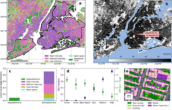
Figure 1. Quantification of developed land covers in the study domain. (a) The 30 m land cover map (Dewitz 2021) shows the distribution of vegetated land covers (i.e. the entire pixel is classified as forest or grasslands) and developed land covers. The developed land covers have four categories—open space, low-, medium-, and high-intensity. The NYC borough boundaries are indicated by black outlines. White color denotes water. (b) The impervious surface area (ISA) fraction. Blue color denotes water. (c) The percentage of vegetated and developed land covers defined in the 30 m land cover map in the study domain. (d) The ISA fraction and enhanced vegetation index (EVI) for different land covers, including deciduous broadleaf forest, grassland, and the four developed land cover categories in the study domain. The symbols denote the averages and the error bars the standard deviations. (e) The 15 cm land cover map for the area highlighted by the red square in panel (b). The grid box denotes the pixel size in the 30 m land cover map.
Download figure:
Standard image High-resolution image2.2. The NYC-VPRM model
We set up a high-resolution (30 m) Urban-VPRM for the study domain. Hereafter, we refer to the model as NYC-VPRM. The equations used in the NYC-VPRM can be found in equations (1)–(8) in the supplementary information. The parameters can be found in table S1 in the supplementary information.
The input data come from publicly available datasets, including enhanced vegetation index (EVI), land surface water index (LSWI), photosynthetically active radiation (PAR), air temperature (Ta), ISA fraction, and the land cover map. The 30 m resolution Landsat EVI and surface reflectance (specifically, near infrared and shortwave infrared bands to calculate LSWI) (Masek et al 2006, Vermote et al 2016) are used in this study. The Landsat swath covering our study domain is Path 13 and Row 32. Both the 16-day Landsat 7 and 8 retrievals were used to create an 8-day dataset of EVI and LSWI. The Collection 2 Tier 1 data of Landsat 7 and 8 are used due to their highest radiometric and positional quality, compared to Tier 2. Pixel quality control was performed to each Landsat scene to select cloud-free pixels. The eight-day EVI and LSWI were then interpolated into daily values for each pixel with a cubic spline function. The 30 m spatial resolution ISA and land cover are from the 2019 National Land Cover Database (Dewitz 2021). The PAR and Ta were extracted from the high-resolution rapid refresh (HRRR, Benjamin et al 2016), a National Oceanic & Atmospheric Administration (NOAA) real-time 3 km resolution, hourly updated atmospheric model. The HRRR 2D surface levels analysis product was used. The 3 km PAR and Ta were linearly resampled into 30 m spatial resolution to match the other input data. Therefore, the NYC-VPRM has a spatial resolution of 30 m and temporal resolution of 1 h.
From our analyses of EVI data, we estimate the start and end of the growing season in our study domain are 15 April and 20 October 2021, respectively (see method in Zhang et al 2003). Because of our focus here on growing season biogenic CO2 fluxes, we ran the NYC-VPRM from 1 April to 31 October in 2021. Note that outside of the growing season when vegetation is not photosynthesizing and soil respiration rates are low, the net biogenic flux is expected to be low (Winbourne et al 2022). We also wanted to avoid the peak pandemic year (2020), where traffic was observed to drop by almost 60% in spring 2020 before recovering to pre-pandemic levels in 2021 (Tzortziou et al 2022). NYC was still the most congested city in the US in 2021 (Wang et al 2021). The summer of 2021 experienced warmer than average Tas in June and August, with two heatwaves in June and one in August. June 2021 was drier than average and was followed by the second wettest July–August on record (figure S1 in the supplementary information).
2.3. Sensitivity analysis of the land cover type in the developed land
Developed land accounts for 90% of the land cover of the study domain (figures 1(a) and (c))—open space, low-intensity, medium-intensity and high-intensity developed areas have impervious surfaces accounting for  20%, 20%–49%, 50%–79%, and 80%–100% of total land cover, respectively. Open space is mostly lawn (Dewitz 2021) and we assume a carbon flux response similar to grassland in the NYC-VPRM because it is the most similar vegetation type for which parameterizations are available. The 15 cm spatial resolution NYC land cover map (https://data.cityofnewyork.us/Environment/Land-Cover-Raster-Data-2017-6in-Resolution/he6d-2qns) suggests that the dominant vegetation type in the low-, medium-, and high-intensity developed land are trees and grass (this product is limited to the five boroughs of NYC). To test the sensitivity of the regional biogenic CO2 fluxes to the vegetation types (i.e. temperate broadleaf forest or grass) assigned to the non-open space developed land (i.e. low, medium, and high intensity) in NYC-VPRM, we designed three experiments (table 1). Hereafter, we refer to the non-open space developed land as developed land for simplicity.
Table 1. The three experiments to test the sensitivity of regional CO2 fluxes to the land cover types assigned to the developed land of low-, medium-, and high-intensity (DEV).
| Experiment | Configuration for DEV | Purpose |
|---|---|---|
| DEVasISA | Treat the non-open space developed land as impervious surfaces | To set the baseline where no contribution of DEV to the regional biogenic CO2 fluxes |
| DEVasDBF | Treat the non-open space developed land as deciduous broadleaf forest | To diagnose the contribution of DEV as deciduous broadleaf forest to the regional biogenic CO2 fluxes |
| DEVasGRS | Treat the non-open space developed land as grassland | To diagnose the contribution of DEV as grassland to the regional biogenic CO2 fluxes |
2.4. Contributions of anthropogenic and biogenic CO2 fluxes to atmospheric CO2
The changes in the atmospheric CO2 concentrations attributed to the anthropogenic and biogenic CO2 fluxes are calculated by combining the Lagrangian atmospheric transport model STILT (the stochastic time-inverted Lagrangian transport model, Lin 2003) with our NYC-VPRM and the monthly sector-specific EDGAR v6.0, emissions for 2018 (Emissions Database for Global Atmospheric Research, Crippa et al
2020) anthropogenic CO2 emission inventory. The STILT model is referred to as HRRR-STILT hereafter as it is driven by the HRRR meteorological data described in section 2.2. HRRR-STILT follows the trajectory of 500 air parcels released from the receptor position (i.e. the Mineola tower in this study) backward in time over the previous 24 h, where the motion of each parcel includes advection by the large-scale wind fields and random turbulent motion, independent of the other parcels. The proportion of particles residing in the lower half of the planetary boundary layer determines the influences of biogenic and anthropogenic CO2 fluxes on the atmospheric CO2 concentrations. The biogenic CO2 fluxes are based on the NYC-VPRM outputs (section 2.2) that are re-sampled to 0.01∘ spatial resolution to match the HRRR-STILT. The anthropogenic CO2 emissions are based on the EDGAR CO2 emission inventory. EDGAR provides the 0.1 spatial resolution emission data from twenty sectors including power industry, combustion, and energy for building on an monthly temporal resolution (figure 2). We focus our analysis on the enhancements in atmospheric CO2 concentrations. The monthly total anthropogenic emissions from EDGAR and the biogenic CO2 emissions estimated by NYC-VPRM can be found in table S2 in the supplementary information.
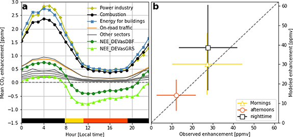
Figure 2. Influences of anthropogenic and biogenic CO2 fluxes on atmospheric CO2 concentrations from 1 April to 31 October 2021. (a) Simulated diurnal variations of the mean CO2 enhancements attributed to individual economic emission sectors and vegetation (both DEVasDBF and DEVasGRS scenarios are shown). Other sectors (gray lines) include oil refinery, aviation landing and takeoff, solvents and products use, chemical processes, aviation climbing and descent, and non-metallic minerals production. (b) The comparison between simulated and observed CO2 enhancements for the period when observations are available (i.e. 11 June–22 July and 9 September–31 October 2021). The symbols and error bars denote the mean and standard deviation of hourly CO2 enhancements, respectively. The time of day is indicated by the yellow, red, and black horizontal bars in figure 2(a).
Download figure:
Standard image High-resolution imageThe calculated CO2 concentration enhancements due to the biospheric fluxes and anthropogenic emissions are evaluated against observations of CO2 at a tower in the suburbs in Mineola, NY (MNY, N40.7495∘, W73.6384∘) relative to CO2 enhancements at the upwind tower in rural Stockholm, NJ (SNJ, N41.1436∘, W74.5387∘) (Karion et al
2020). The observed CO2 concentrations are available at both sites for the period of 11 June–22 July and 9 September–31 October in 2021. The prevailing wind direction is from the west and thus Mineola is downwind of Stockholm. The small vertical gradients in CO2 concentrations at Stockholm suggest little impacts by local fluxes either biogenic or fossil due to high elevation. We use the afternoon averages over a three-day period of CO2 data at Stockholm as the background concentrations (Sargent et al
2018). The observed hourly CO2 concentration enhancements are then estimated as the hourly [CO2] –background [CO2]
 .
.
3. Results and discussion
3.1. The dominance of the developed land covers in NYC
Developed land cover categories (including open space) account for 90% of the total land area of the study domain, while vegetation categories comprise the remaining 10% (figures 1(a) and (c)). The medium- and high-intensity developed land accounts for 70% of the total land area while low-intensity and developed open space cover 20% of the land area. The EVI for the developed land can be considerable in the summer months (figure 1(d)), highlighting the high amount of vegetation that occurs in these land cover categories (figure 1(e)). For example, the EVI of developed open space is comparable to the EVI of grassland land covers, and can be as high as 0.7 (figure 1(d)). Because developed land covers can have relatively high EVI values (i.e. vegetation cover), we find they dominate the regional urban biogenic CO2 fluxes in the study domain.
3.2. Sensitivity analysis of land cover type in the developed land
3.2.1. Vegetation or no vegetation?
We find that vegetation in the developed land contributes significantly to the region's biogenic CO2 fluxes (i.e. GEE, Res, and net ecosystem exchange NEE = GEE + Res) during the summer (figure 3(a)). Specifically, compared to assumptions of no vegetation in the developed land covers, the regional total GEE increases by three (from 0.1 to 0.27 TgC month−1) and four fold (from 0.1 to 0.38 TgC month−1) when vegetation in the developed land is treated as forest or grassland, respectively, and total Res (heterotrophic + autotrophic) increased by factors of 6 (from 0.02 to 0.12 TgC month−1) and 2 (from 0.02 to 0.04 TgC month−1), respectively. Altogether, these enhanced biogenic CO2 fluxes result in a 2–4 times (from 0.08 to 0.17 or 0.34 TgC month−1) increase in regional NEE when taking into account the vegetation in the developed land (figure 3(a)). These findings indicate that assuming zero biogenic CO2 fluxes from vegetated developed land, which is common in larger-scale weather and climate models, can lead to a significant underestimation of regional biogenic CO2 fluxes in urban environments (figure S2 in the supplementary information).
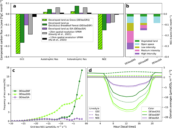
Figure 3. Sensitivity of regional biogenic carbon fluxes to land cover types in NYC-VPRM for June 2021. (a) The modeled total gross ecosystem exchange (GEE), autotrophic and heterotrophic respiration (Res), and net ecosystem exchange (NEE) across the study domain for June 2021. The modeled fluxes from a ∼2 km VPRM and a 12 km VPRM coupled in the Weather Research and Forecasting Model are also shown for comparison. (b) The contributions of different land cover types to the regional NEE. (c) The frequency of occurrence of the grid-box NEE values across the study domain (i.e. ratios of the number of pixels within a certain NEE range to the total number of pixels in the domain). (d) The diurnal variations of the domain-averaged NEE.
Download figure:
Standard image High-resolution imageVegetation in the developed land covers of low-, medium-, and high-intensity contributes differently to the regional NEE across the domain. Medium-intensity development accounts for a higher portion of land area in the study domain relative to low-intensity (30% versus 12%, figure 3(c)) and makes a larger contribution to EVI compared to high-intensity (0.28 versus 0.14, figure 3(d)), thus contributing most to total NEE in the domain. In general, given the predominance of the developed land in the study domain ( 90%), the vegetation within the developed land cover categories (e.g. lawns and trees in parks, yards, and along streets) dominates the domain's total NEE. The conventional ecosystem land cover categories of 'forest' and 'grassland', that only account for
  10% of the domain area collectively, contribute roughly 15% to the regional NEE in our study domain (figure 3(b)).
3.2.2. Grassland or tree?
Because of large differences in CO2 fluxes between grassland and deciduous broadleaf forest ecosystems, we find that the simulated regional biogenic carbon fluxes are quite sensitive to how the vegetation within developed land covers is categorized (figure 3(a)). Specifically, the regional total GEE, Res, and NEE vary by a factor of 1.4, 0.4, and 2.2, respectively, between the two scenarios (figure 3(a)). The 15 cm spatial resolution NYC land cover map suggests that the tree and grass coverage are roughly the same in the low-intensity developed land and the tree coverage in the medium- and high-intensity developed land (25% and 11%) is higher than grass (16% and 5%). Overall, the relative contribution of trees to total vegetation cover, relative to grass, increases as development density increases. Note that the 15 cm land cover map only covers the political boundaries of NYC which comprises 65% of our study domain. The developed land cover categories outside of NYC in our study domain are dominated by open space and low-intensity developed land cover categories (figure 1(a)) and therefore likely contain more urban grassland (i.e. lawn) than developed land within NYC itself. As such, we expect our DEVasDBF and DEVasGRS scenarios (figure 3) to be bookend estimates of the actual biogenic CO2 fluxes across our study domain, with the actual fluxes being somewhere between the estimates derived from these two scenarios.
3.2.3. Lawn or grassland?
Lawns (i.e. urban grasslands)—which are typically composed of both grasses and herbs—are oftentimes the most common herbaceous plant-dominated ecosystem type in cities and developed landscapes (Ignatieva et al
2015). However, there are currently no model parameters specifically for 'urban grasslands.' Here, we use 'grassland' model parameters that derived from the Vaira Ranch Grassland in California which is dominated by C3 annual grasses and herbs. The plants in this ecosystem with a Mediterranean climate are functional during the winter and early spring and dead during the summer (Xu and Baldocchi 2004). There are obvious differences in climate, environmental conditions, and management between a rural grassland system in California and an urban grassland in NYC. First, the ecosystem respiration of Vaira grasses is mainly driven by precipitation and shows higher respiration rates during wet and cooler season (Xu and Baldocchi 2004), suggesting a weakened relationship with Tas. However, urban lawns under management such as irrigation likely show a stronger temperature-respiration relationship, compared to the unmanaged Vaira Ranch grasses. This could lead to an underestimation of lawn ecosystem respiration by VPRM. Second, Vaira grassland has similar drivers as urban grasslands for gross primary production (GPP)—Ta, light intensity, and leaf area index (Xu and Baldocchi 2004, Miller et al
2018). Miller et al (2018) report a GPP of  ± 1.0 gC m−2 d−1 for turf grasses and Xu and Baldocchi (2004) 4.5–5.0 gC m−2 d−1 for Vaira grasses, suggesting that the parameterization of Vaira grasses based on Xu and Baldocchi (2004) might provide a reasonable estimation of GPP for lawns. That said, the obvious differences in climate and grass community composition between Vaira and lawns in mesic temperate cities highlight the need for development of model parameterizations for urban lawns. Miller et al (2018) report an empirical light use efficiency for low-maintenance lawns, but more than 50% of homeowners fertilize their lawns (Polsky et al
2014). Parameterization for GPP and ecosystem respiration for lawns of different levels of management is still lacking. Our results highlight the need to develop a more comprehensive set of empirical parameters for urban grasslands using both site-specific and regional gridded input data sets.
± 1.0 gC m−2 d−1 for turf grasses and Xu and Baldocchi (2004) 4.5–5.0 gC m−2 d−1 for Vaira grasses, suggesting that the parameterization of Vaira grasses based on Xu and Baldocchi (2004) might provide a reasonable estimation of GPP for lawns. That said, the obvious differences in climate and grass community composition between Vaira and lawns in mesic temperate cities highlight the need for development of model parameterizations for urban lawns. Miller et al (2018) report an empirical light use efficiency for low-maintenance lawns, but more than 50% of homeowners fertilize their lawns (Polsky et al
2014). Parameterization for GPP and ecosystem respiration for lawns of different levels of management is still lacking. Our results highlight the need to develop a more comprehensive set of empirical parameters for urban grasslands using both site-specific and regional gridded input data sets.
3.2.4. High spatial heterogeneity
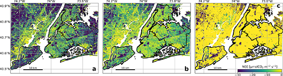
There is considerable spatial variability of NEE across the domain (figure 4). Throughout June, NEE values at some locations approach −30 µmol m−2 s−1 (figure 3(c)), which is comparable to the Eddy-covariance observations in Harvard forest (Urbanski et al 2007). The NEE from developed land when all vegetation is assumed to be trees, ranges from −10 to 0 µmol m−2 s−1. In contrast, when the vegetation in developed land is assumed to be grassland, the NEE exhibits a wider range from −25 to 0 µmol m−2 s−1 with a higher frequency of more negative values. This large spatial heterogeneity of the biogenic carbon fluxes across the domain is often not captured by large-scale models with coarser spatial resolutions (Hu et al 2021, Gourdji et al 2022). Measurements of biogenic CO2 fluxes from different urban ecosystems (e.g. lawns, urban savannas, fragmented forests, etc) and across seasons are needed to evaluate model results and improve performance of carbon flux models in urban landscapes. The domain-averaged GEE and NEE show typical diurnal variations with maxima around noon in all three scenarios, as well as the differences between cases (figure 3(d)).
Figure 4. A map of modeled net ecosystem exchanges (NEEs) at local noon on 27 June 2021. NEE from the three experiments are shown, including treating the non-open space developed land as grassland ((a) DEVasGRS), as deciduous broadleaf forest ((b) DEVasDBF), as impervious surfaces ((c) DEVasISA).
Download figure:
Standard image High-resolution image
3.3. Influences of biogenic and anthropogenic fluxes on atmospheric CO2
3.3.1. Simulated and observed atmospheric CO2 enhancements
The simulated atmospheric CO2 enhancements agree well with the observed CO2 enhancement, especially during the daytime, when the boundary layer is well mixed (figure 2(b)). The key factors that impact the agreement include (a) correctly capturing the boundary layer dynamics in the Lagrangian atmospheric transport model STILT, (b) accurately defining the upwind background CO2 concentrations (see details in section 2.4), and (c) accurate representation of the biogenic and anthropogenic surface CO2 fluxes. We observe large day-to-day variability in the simulated CO2 enhancements, likely driven by boundary layer dynamics such as wind and mixing conditions (figure 2) and more variability at night when the low nocturnal boundary layer magnifies the enhancement from biogenic respiration and anthropogenic CO2 emissions. The first two factors above have been extensively studied and tested (e.g. Sargent et al 2018) allowing us to assess the impact of the biogenic and anthropogenic fluxes. The overall good agreement in this study highlights that a detailed representation of urban biological fluxes and knowledge of the spatial and temporal distribution of emissions are essential for detecting variability in atmospheric CO2 concentrations.
The atmospheric CO2 concentration enhancements are, on average, 30 ppmv in the morning and 12 ppmv in the afternoon (figure 2(b)), while nighttime enhancements are larger due to the shallow nighttime stable boundary layer. This diurnal variation in atmospheric CO2 enhancements can also be seen in figure 2(a). The large variability in morning and nighttime CO2 enhancements manifests challenges in both measurements and modeling under stable boundary layer conditions. In the following discussion, we focus on the afternoon period when the boundary layer is well-mixed.
3.3.2. Biogenic and anthropogenic influences
During summer afternoons, vegetation uptake of CO2 across our study domain is large enough to completely offset the respective CO2 concentration enhancements produced by many of the individual (i.e. not the sum) anthropogenic sectors such as energy for buildings, the power industry, combustion for manufacturing, or on-road traffic (figure 2(a)). Depending on the vegetation type assumed for the developed land (i.e. the DEVasDBF or DEVasGRS scenario), NEE offsets 20%–40% of CO2 emissions attributed to total anthropogenic emissions during summer afternoons. While these offsets are for the most photosynthetically active time of year, and thus an upper limit of carbon offset possible from urban vegetation, we find it surprising that even in a city with the development density and CO2 emissions as high as NYC, vegetated systems still make a large contribution to urban CO2 fluxes. This large biogenic flux greatly confounds attempts to quantify city-wide carbon budgets, resulting in much greater uncertainty.
NYC has the third largest anthropogenic CO2 emissions globally (Moran et al 2018) and has a relatively low tree canopy coverage of only 22% (Treglia et al 2021). The Boston urban region has a similar climate and a tree canopy of 25% (Raciti et al 2014) as NYC, but lower citywide anthropogenic CO2 emissions of 0.92 kgC m−2 yr−1 (Sargent et al 2018) compared to 9.4 kgC m−2 yr−1 in our study domain (based on EDGAR). Sargent et al (2018) found that biogenic uptake almost completely balances anthropogenic CO2 emissions on summer afternoons in Boston. Given the similar tree canopy cover and ten times higher anthropogenic emissions in our study domain, one might expect the vegetation to offset roughly 10% of emissions, all else being equal. However, our results suggest a vegetation offset between 20% and 40% on summer afternoons (e.g. figure 2). The importance of biogenic CO2 fluxes in mediating urban enhancements of CO2 even in a city of low tree canopy cover as NYC underscores the large impacts of biology on carbon cycling for cities of all sizes, particularly as many move to increase vegetation cover. The biogenic CO2 fluxes should be accurately evaluated as carbon mitigation policies are introduced.
We find that CO2 enhancements by on-road traffic could be entirely offset by vegetation uptake in a summer afternoon, which indicates that biogenic fluxes become more important when using top-down approaches for quantifying emissions from individual economic sectors. The transportation sector generates the largest share (27%) of greenhouse gas emissions nationwide, followed by electricity (25%), industry (24%), commercial & residential (13%), and agriculture (11%) (EPA 2022). Although the on-road traffic is overwhelmed by power industry and energy for buildings due to its geographic proximity to a number of power plants and old building infrastructure respectively, NYC is still the most congested city in the US in 2021 as traffic levels are beginning to increase again compared to pre-pandemic levels in 2019 (Wang et al 2021). EDGAR suggests on-road traffic accounts for 10% of total anthropogenic CO2 emissions, but a more recent emission inventory (Gately and Hutyra 2022) estimates a higher share (25%) in NYC. As the vegetation offsets up to twice the CO2 enhancements by on-road traffic in the most congested NYC, we expect this is also the case for less congested cities especially with an increasing electric car share.
The net sign of biogenic CO2 fluxes exhibits large diurnal and seasonal variations (e.g. large uptake during summer daytime) (figures 2(a) and (c)) that are relevant to accurate assessment of carbon mitigation policies. Remotely sensed variability in atmospheric CO2 concentrations are often used to validate 'bottom-up' methods and to evaluate the carbon mitigation policies. However, these satellites pass the urban areas at a certain time of day, often in the afternoons when the biogenic influences on the CO2 concentrations are strongest. Therefore, an accurate assessment of changes in observed atmospheric CO2 concentrations attributed to anthropogenic emissions needs to tease out the influences of biogenic CO2 fluxes.
4. Conclusion
Even in large, dense cities like NYC, summertime biogenic CO2 fluxes can be large relative to anthropogenic emissions. Vegetation in developed land cover categories, rather than more conventional ecosystems like forests and grassland, overwhelmingly drive the biogenic CO2 fluxes in NYC. Regional biogenic CO2 fluxes in NYC can be significant, contributing 46%–76% of the total biogenic carbon in the metro area depending on the plant functional type. These urban biosphere carbon fluxes are rarely accounted for in regional models. Developed land covers are ubiquitous in cities and vegetation in these developed areas often exists in the form of street trees, park trees, and lawns. Accurate estimates of biogenic CO2 fluxes in an urban context require high-resolution, spatially resolved land cover datasets to capture the high heterogeneity in land cover types and vegetation cover. Vegetation type in developed land covers has a large influence on city-wide estimates of biogenic CO2 fluxes, so future measurements should focus on constraining understanding of CO2 fluxes in urban grasslands (i.e. lawns) because there is no natural analog to these systems.
Despite NYC having the largest anthropogenic CO2 emissions of any city in the US and containing relatively little vegetation cover, biogenic CO2 uptake still offsets up to 40% of the city's CO2 enhancements from anthropogenic emissions on summer afternoons. This highlights the important contribution urban ecosystems make to urban carbon cycling, even in large megacities. With a growing number of cities embracing ambitious carbon emission reduction goals, there is a rapidly growing need for tools to assess a city's progress towards these goals. Accurate characterization of the vegetation and biogenic carbon fluxes of a city's ecosystems are essential to the development of effective atmospheric monitoring tools.
Data availability statement
The NYC-VPRM and HRRR-STILT outputs are available at Dryad (https://doi.org/10.5061/dryad.4j0zpc8f2). The hourly CO2 data at Stockholm, NJ and Mineola, NY can be found in Karion et al (2022) (https://doi.org/10.18434/mds2-2649). The Landsat EVI and LSWI can be downloaded at https://espa.cr.usgs.gov. The HRRR PAR and Ta data can be downloaded at https://www.nco.ncep.noaa.gov/pmb/products/hrrr. The data that support the findings of this study will be openly available following an embargo at the following URL/DOI: https://doi.org/10.5061/dryad.4j0zpc8f2.
Acknowledgment
We acknowledge support by National Oceanic and Atmospheric Administration under Grant NA20OAR4310306. We acknowledge Anna Karion (The National Institute of Standards and Technology) for providing the CO2 concentration data at Mineola, NY and Stockholm, NJ.
Supplementary data (0.7 MB PDF)