
Abstract
Water is one of the most critical resources derived from natural systems. While it has long been recognized that forest disturbances like fire influence watershed streamflow characteristics, individual studies have reported conflicting results with some showing streamflow increases post-disturbance and others decreases, while other watersheds are insensitive to even large disturbance events. Characterizing the differences between sensitive (e.g. where streamflow does change post-disturbance) and insensitive watersheds is crucial to anticipating response to future disturbance events. Here, we report on an analysis of a national-scale, gaged watershed database together with high-resolution forest mortality imagery. A simple watershed response model was developed based on the runoff ratio for watersheds (n = 73) prior to a major disturbance, detrended for variation in precipitation inputs. Post-disturbance deviations from the expected water yield and streamflow timing from expected (based on observed precipitation) were then analyzed relative to the abiotic and biotic characteristics of the individual watershed and observed extent of forest mortality. The extent of the disturbance was significantly related to change in post-disturbance water yield (p < 0.05), and there were several distinctive differences between watersheds exhibiting post-disturbance increases, decreases, and those showing no change in water yield. Highly disturbed, arid watersheds with low soil: water contact time are the most likely to see increases, with the magnitude positively correlated with the extent of disturbance. Watersheds dominated by deciduous forest with low bulk density soils typically show reduced yield post-disturbance. Post-disturbance streamflow timing change was associated with climate, forest type, and soil. Snowy coniferous watersheds were generally insensitive to disturbance, whereas finely textured soils with rapid runoff were sensitive. This is the first national scale investigation of streamflow post-disturbance using fused gage and remotely sensed data at high resolution, and gives important insights that can be used to anticipate changes in streamflow resulting from future disturbances.
Export citation and abstract BibTeX RIS
1. Introduction
Water is one of the most critical environmental resources and is tightly linked to landscape composition (ecology), soils, and land cover change. Forested watersheds in particular are important as natural water sources for residential, commercial, and agricultural needs around the world [NRC 2008]. But despite a long appreciation of the significance of forests to water supplies, the effect of forest disturbances (e.g. wildfire, insect outbreaks) on water yield remains difficult to predict [Hibbert 1967, Postel and Thompson 2005, Neary et al 2009] and is a highly interdisciplinary problem, incorporating aspects of biology, geology, soil sciences, climatology, and hydrology. This complexity is reflected in the variety in published research; with regard to post-disturbance streamflow yield, many studies report increases in yield [Sahin and Hall 1996, Wondzell and King 2003, Brown et al 2005, Buma and Livneh 2015] but several find little change or a decrease in yield [e.g. Adams et al 2012, Biederman et al 2012, Biederman et al 2014, Brantley et al 2014, Biederman et al 2015] or increased yield transitioning to decreased after a decade or more post-disturbance [Hornbeck et al 1997]. In this context water yield is defined as the total annual runoff from a watershed as measured in a stream, i.e. total streamflow. In addition, while much of the attention historically has focused on sensitive watersheds, it is equally interesting to understand why some watersheds are insensitive to major disturbances which may cause substantial streamflow changes in other locations [e.g. in the context of streamwater nitrate loss, Rhoades et al 2013]. Knowing which watersheds are likely insensitive is a means to save managerial resources for future needs elsewhere. Anticipated changes in the future prevalence of disturbances [Dale et al 2001] highlights the need for a clearer understanding of which watershed features are associated with sensitivity to these events.
Vegetation exerts important controls on the hydrological functioning of most watersheds through a variety of mechanisms that impact water inputs, outputs, and flux rates [Jorgenson and Gardner 1987, Schleppi 2010]. The relationship between forest disturbances and resulting hydrologic impacts has a long research history spanning a broad range of ecosystems [McCulloch and Robinson 1993] with increasing frequency in recent decades [Hibbert 1967, Bosch and Hewlett 1982, Zhang et al 2001, Naranjo et al 2011].
The catchment water balance, and broad drivers of its change, were formalized by Horton [1933] and have received substantial attention since. Forest have an important influence on catchment water balance. Precipitation input into a catchment (fog, rain, and snow) is modulated by canopy interception and incoming/outgoing radiation are further affected by that canopy [Gustafson et al 2010, Harpold et al 2014, Veatch et al 2009], influencing sublimation and evaporation processes within and below the canopy [Rinehart et al 2008, Simonin et al 2009, Boon 2012, Pugh and Gordon 2013]. Belowground, tree roots alter soil properties, typically increasing infiltration and lowering the potential for evaporation [Jorgensen and Gardner 1987, Federer et al 2003, Guswa 2012, Miller and Zegre 2014]. Once water infiltrates into the watershed soils, vegetative transpiration is a dominant water flux from many catchments [Biederman et al 2015, Jasechko et al 2013], though discharge can be more significant in humid/wet systems. Forests in particular lose a greater fraction of their annual precipitation to transpiration than lower biomass systems, i.e. grasslands [Zhang et al 2001]. Therefore, because forests are strong drivers of transpiration and because their spatial distribution is often driven by patterns of water availability [Thompson et al 2011], disturbance and vegetation change are critical components of streamflow patterns.
Although conceptual models have been put forward that relate vegetation disturbance with hydrological response [e.g. Pugh and Gordon 2013], the majority of empirical research has been limited to paired catchment studies, numerical modeling, and syntheses [Schleppi 2010, Mikkelson et al 2013, Sahin and Hall 1996, Livneh et al 2015]. Brown et al (2005) provide a review of studies exploring the response of different forest types (conifer, deciduous, scrub) to clear-cutting disturbance, identifying characteristic responses for each forest type, and reporting an overall increase in water yield observed in response to forest loss. Experimentation in a moist temperate forested area [Hibbert 1967] demonstrated that streamflow generally increased proportionally with the degree of forest harvest. However, substantial temporal variations in this relationship have been reported there and elsewhere with streamflow increases strongly influenced by topographic characteristics [e.g. slope; Voepel et al 2011] and related effects such as changes in solar radiation [e.g. Douglass 1983]. While disturbances alter the relative partitioning between total evaporation and transpiration losses through a variety of site specific conditions, water yield increases are often attributed to reduced transpiration with less forest cover post-disturbance [Sahin and Hall 1996, Andreassian 2004]. Supporting this hypothesis, growth of vegetation has a negative effect on streamflow. A survey of ten catchments in the US piedmont region showed that 10%–28% increases in forest cover led to increased ET and reduced water yield by between 4%–21% [Trimble et al 1987]. Projections across China have similarly suggested post-afforestation declines of 10%–50% in water yield based on statistical landcover ET-precipitation relationships [Sun et al 2006]. Studies like Kuczera [1987] and Brookhouse et al [2013] report that as forests recover from disturbance, subsequent increases in water yield diminish and over time (> 10 years) can eventually reverse, becoming decreases in water yield below undisturbed levels, attributed to early successional vegetation with higher ET rates [Hornbeck et al 1997]. Overall, the majority of studies have posited that reduced transpiration driven by mortality [e.g. Schäfer et al 2014] should overwhelm the other mechanisms, leading to increases in water yield and earlier streamflow post-disturbance.
Importantly, various exceptions to the expectation of increased water yield post-disturbance have been published recently. Some watersheds are relatively insensitive to disturbance, meaning little change is noted despite substantial vegetation change. This has been attributed to other drivers overwhelming the transpiration response, such as climate [e.g. Hallema et al 2016]. Unanticipated decreases in water yield post-disturbance have been attributed in part to regrowth of water-intensive understory vegetation and evaporation [Adams et al 2012, Biederman et al 2014, Biederman et al 2015, Fernandez et al 2006, Guardiola-Claramonte et al 2011]. Similarly, conflicting shifts in streamflow timing have been reported (i.e. changes in the date at which a given fraction of annual streamflow is observed). Several disturbance-mediated mechanisms have been identified that influence these changes, such as changes to infiltration and base-flow [Bruijnzeel 1988], soil compaction [Miller and Zegre 2014], net transmission of solar radiation [Pugh and Gordon 2013], and hydrophobicity/reduced porosity from fires [Wondzell and King 2003].
Predicting the sign of the water yield and timing change post-disturbance remains an open problem. Recent attempts at prediction have taken multiple approaches, such as portioning streamflow into fast and slow groups which have different responses to disturbance [Harman et al 2011], developing new indices [e.g. rain use efficiency, Troch et al 2009, Thompson et al 2013], or tying response to climate in some fashion [e.g. aridity: Budyko 1974, storminess: Milly 1994]. Applications of indices over large numbers of catchments have had mixed results due to complex topographic and climate interactions [Voepel et al 2011]. To date, no single feature has been identified capable of predicting the direction of watershed hydrologic sensitivity to disturbance.
To address this gap, we developed a simple model to predict change in water yield and streamflow timing post disturbance. First, we describe the shift in water yield or timing using a detrended version of runoff ratio (yield) and the centroid of yearly flow (timing; described as Julian date) which incorporates variable precipitation inputs and historical records. In situ and remotely sensed historical data were used to identify characteristic traits of sensitive and insensitive watersheds, using a large, continent spanning set of historical streamflow data. The unique perspective presented here is an evaluation of deviations from assumed precipitation-hydrology relationships across a range of disturbance amounts and vegetation types. Understanding which watersheds are likely sensitive to disturbance will ultimately enable better proactive management of water and forests [Douglass 1983, Thompson et al 2013] by enabling more informed allocation of limited managerial resources.
Our primary research goal is identifying what watershed characteristics are associated with either sensitivity to disturbances or insensitivity (no major change) in terms of both yield and streamflow timing.
2. Data sources and methodology
For a flowchart of processing steps, see figure M1. Among the 671 United States Geological Survey (USGS) watersheds identified as best representing natural flow [Newman et al 2015, Lins 2012], initial consideration was restricted to the 228 that are undammed, while development of the statistical modeling component was further restricted to 73 that experienced substantial disturbance during the time-period of observation (> 1% disturbed area, see below and supplementary methods available at stacks.iop.org/ERL/12/074028/mmedia). The area disturbed in each watershed was quantified on a yearly basis (2001–2010) using yearly, 30 m resolution maps of forest disturbance [Hansen et al 2013]. We then identified the year of the largest disturbance (total area) and focused on changes in water yield and streamflow timing in the subsequent water year (water year = 1 Oct. through 30 Sep.); as a result, if the largest disturbance year was 2010 the watershed was discarded. The year of largest forest disturbance and subsequent hydrologic response was chosen for two reasons: First, it did not constrain our focus to a single minimum cutoff disturbance extent across the entire dataset, which represents a diversity of disturbance drivers and landscapes. Second, focusing on the hydrologic response in the subsequent year allowed for clarity in the drivers of immediate hydrological change, before ecological communities have significant time to recover (though partial recovery within a single year cannot be excluded). Other drivers, such as dominant species shifts in response to the disturbance, may become significant in later years.
2.1. Simple model of expected water yield and streamflow timing change post disturbance
GIS maps of watershed boundaries [Newman et al 2015] were combined with precipitation from Daymet [Thornton et al 2014] and observed streamflow data from the USGS. Expected water yield from a watershed is commonly assessed using the Runoff Ratio (RR = total streamflow/total precipitation; figure 1). Runoff ratio is a means to standardize between watersheds of very different sizes and precipitation amounts by relating precipitation to water yield. Importantly, runoff ratio and streamflow timing can vary with precipitation, and the response is different between disturbed and undisturbed watersheds as demonstrated in Brown et al [2005]. Therefore, we first detrended the runoff ratio by observed precipitation to account for ratio variability as a function of precipitation. We developed a simple linear regression model of the expected detrended runoff ratio and streamflow timing for years prior to the disturbance. The observed runoff ratio post-disturbance was compared to expected runoff ratio, calculated using the pre-disturbance regression model and observed precipitation, to create the detrended residual runoff ratio (dRRR)—the amount by which the actual runoff ratio differed from expected in the absence of a disturbance and given the observed precipitation in the year immediately following the disturbance. This is our measure of sensitivity; i.e. deviation from expected behavior.
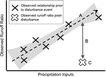
Figure 1 Creation of the detrended runoff ratio, RR, response variable. All years prior to the disturbance were used to model the observed precipitation—runoff ratio relationship. For the year following the disturbance, the expected RR was calculated based on observed precipitation (A). Actual runoff (C) was then subtracted from (A), leaving (B), the residual from expected (dRRR). The meaningfulness of the residual runoff ratio departures, dRRR, was verified against the expected historical range of variability using an independent preceding period, 1985–2000. An identical procedure was repeated for streamflow timing change based on changes in the centroid date of streamflow post-disturbance.
Download figure:
Standard image High-resolution image2.1.1. Grouping watersheds
Selecting watersheds for the final analysis was a two-step process, involving grouping all watersheds into general post-disturbance response groups (streamflow: increasing, insensitive, or decreasing; timing: earlier, insensitive, later) and then sub-setting to highly disturbed watersheds. First, undammed watersheds (n = 228) were grouped into three categories based on post-disturbance behavior: sensitive (increasing or decreasing) or insensitive. The watersheds were divided by percentiles based on hydrologic response—those that experienced large decreases in water yield (bottom 25%, dRRR highly negative [mean −18% change in RR from expected]), those that were relatively insensitive (middle 50%, dRRR approximately zero [mean + 0.1% change in RR]), and those where water yield increased (top 25%, dRRR highly positive [mean + 13% change in RR]; figure S1). Finally, since not all the watersheds experienced a major disturbance during the time period of observation, only watersheds with a disturbance exceeding 1% of their total area in at least one year were retained; 32% of the undammed watersheds met this criterion (final n = 73; 14 in the decreasing yield group, 37 in the insensitive group, and 22 in the increasing yield group). All watersheds in the negative group showed a decline in RR, all watersheds in the positive group show an increase, and the insensitive group showed little deviation from expected (table 1). The watersheds were well distributed spatially with a range of drainage areas (mean = 399 km2, SD = 582 km2), climates (annual precipitation: mean = 1430 mm, SD = 740 mm; annual temperature: mean = 10.3 °C, SD = 5.4 °C), and land cover types (figure S2).
Table 1. Characteristics of the final groups for the discriminant analysis (n = 73).
| dRRR (difference in RR from expected) | Centroid timing change (days) | |||||
|---|---|---|---|---|---|---|
| Group | Min | Mean | Max | Min | Mean | Max |
| Decreasing | −0.45 | −0.14 | −0.05 | −103 | −19 | −45 |
| Insensitive | −0.04 | 0.01 | 0.06 | −18 | −2 | 13 |
| Increasing | 0.06 | 0.13 | 0.34 | 14 | 37 | 173 |
The fact that the magnitude change of the decreasing group is of similar magnitude to the increasing group represents a departure from the expectation of previous paired-catchment work (e.g. Bosch and Hewlett 1982) and instead is more in line with newer studies such as Guardiola-Claramonte et al [2011] that use a pre- and post-disturbance runoff ratio approach and find decreases in streamflow in some cases. Our method calculates a detrended runoff ratio residual, which although similar to the latter study, is unique, since it considers and controls for the influences of wet and dry years (known to influence runoff ratio) on streamflow response.
Partitioning into response groups was done based on the relative magnitude of streamflow change rather than a statistical threshold because of the limited number of years of satellite disturbance data [Hansen et al 2013], extending back only to 2000. This meant watersheds had differing numbers of years prior to the disturbance from which to develop our model. For example, a major disturbance in 2007 would result in 6 prior years of runoff-ratio data versus a disturbance in 2005, which would have 4 prior years. The asynchronous effect of disturbance and data availability complicate subsequent statistical analysis of the response groups (variable statistical power), although we report the significance of the changes in streamflow relative to historical variability in the next section. Furthermore, we use percentile groupings (positive, no change, negative) rather than simple percentage thresholds (e.g. >−5%, −5 to + 5%, and >5% change in RR) to avoid making arbitrary numerical cutoffs in the data. However, the end result was balanced, as the percentile cutoffs were −0.45% and +0.5% for the decreasing and increasing yield groups respectively (table 1).
As a secondary check that the sensitive groups (increased or decreased yield) were associated with substantial changes in historical streamflow amount or timing, we constructed an estimate of detrended runoff ratio variability for each watershed from 1985 to 2000 as a control. Linear precipitation-RR relationships for each watershed were used to calculate the expected 95% prediction interval. We then compared the observed post-disturbance RR and precipitation to verify that the post-disturbance RR change was outside the expected RR range of variability using the control 1985–2000 time period. 93% of the watersheds with decreased streamflow post-disturbance were outside the 1985–2000 precipitation-RR relationship inter-annual variability envelope whereas 60% of the watersheds with increasing streamflow were outside the interval. This indicates that the grouping based on percentiles is statistically meaningful; in other words, the majority of the increasing and decreasing response groups were significantly different from their historical norms, regardless of the proportion disturbed.
Streamflow timing change was calculated in an identical way as RR, except using the centroid of the runoff response: the date each year on which 50% of daily flow had been observed. The same detrending and grouping procedure based on percentiles was employed for streamflow timing yielding an earlier group (mean 47 days before expected, n = 20), no change (mean 3 days before expected, n = 34), and later group (mean 51 days after expected, n = 19, figure S1).
2.1.2. Model development
To identify watershed characteristics which differentiated sensitive from non-sensitive watersheds, we associated post-disturbance watershed response with 75 vegetative, climatic, soil, and disturbance characteristics [Falcone et al 2010] in a linear discriminant analysis (LDA) framework. A complete description of the predictor variables, including how they are calculated and original data sources, are in table S1. The LDA methodology is a supervised technique which uses groups identified a priori (the three post-disturbance response groups) and identifies which linear combination of variables best differentiates between those groups. However, because the LDA methodology is sensitive to the range of variability and correlation across variables, two preliminary steps were taken. First, variables were scaled (normalized) giving them a mean value of zero and standard deviation of one. Second, to reduce the inter-correlation and total number of potential explanatory variables, group membership was modeled using the Random Forests technique [Breiman 2001]. The top 25 most explanatory variables from that framework were then used in the LDA analysis. This was done separately for water yield and streamflow timing, resulting in different potential variables for each.
The final 25 variables were combined via the LDA to determine the most significant features which differentiate one response group from another using the caret package in R (Kuhn 2008). To assess if final groupings were significantly different from each other Kruskal–Wallis nonparametric tests were used. A detailed methodology, including full variable selection procedures, is found in Supplementary Methods.
3. Results and discussion
Both water yield changes and streamflow timing showed relationships to disturbance, but in different contexts and with differing magnitudes (examples: table 2). The majority of disturbed watersheds displayed either little change (n = 37) or an increase in streamflow (n = 22), with a minor component showing streamflow declines (n = 14). The strongest predictors of group membership are shown in figure 2. Overall classification accuracy was 84% for predicting water yield change (95% confidence interval: 73.1%–91.2%), and significantly better than the null hypothesis of no response (p < 0.00001) and 74% for predicting streamflow timing change (95% confidence interval: 0.62%–0.84%, p = 0.003).
Table 2. Examples of both highly and lightly disturbed watersheds used in the final analysis. The USGS stream gage ID and approximate location are included. Watershed characteristics are a subset of all the characteristics that were considered in the development of the model. For all variables, see supplementary data for distributions and the GAGES-II database (Falcone et al 2010) for complete derivation methods.
| ID | Lat. | Long. | Disturbed percent | Drainage size (km2) | Mean Precip. (cm) | Contact time (days) | Fragment-ation Indexa | Deciduous cover (percent) | dRRR | Timing change (days) | Group for yield | Group for timing |
|---|---|---|---|---|---|---|---|---|---|---|---|---|
| 11098000 | 34.2 | −118.2 | 0.62 | 41.60 | 78.85 | 6.50 | 16.60 | 0.00 | 0.10 | −1.38 | Increase | Insens. |
| 12447390 | 48.8 | −120.1 | 0.62 | 58.10 | 88.33 | 13.40 | 3.00 | 0.00 | −0.01 | −35.09 | Insens.b | Earlier |
| 12374250 | 47.8 | −114.7 | 0.56 | 50.80 | 57.97 | 16.10 | 3.00 | 0.00 | 0.13 | 7.39 | Increase | Insens. |
| 11124500 | 34.6 | −119.9 | 0.50 | 191.50 | 83.10 | 26.40 | 3.50 | 0.01 | 0.15 | −28.49 | Increase | Earlier |
| 13235000 | 44.1 | −115.6 | 0.03 | 1163.20 | 101.19 | 16.80 | 2.30 | 0.42 | 0.03 | 5.96 | Insens. | Insens. |
| 08269000 | 36.4 | −105.5 | 0.03 | 163.30 | 63.82 | 8.50 | 1.70 | 5.13 | −0.02 | 10.72 | Insens. | Insens. |
| 14222500 | 45.8 | −122.5 | 0.03 | 323.90 | 334.17 | 49.40 | 9.90 | 2.34 | −0.04 | −9.20 | Insens. | Insens. |
| 07340300 | 34.4 | −94.2 | 0.01 | 230.40 | 157.30 | 83.60 | 9.20 | 58.97 | −0.18 | 14.66 | Decrease | Later |
| 02381600 | 34.6 | −84.5 | 0.01 | 10.30 | 159.91 | 50.80 | 38.30 | 70.21 | −0.23 | −20.10 | Decrease | Earlier |
| 14306500 | 44.4 | −123.8 | 0.01 | 857.20 | 210.88 | 26.00 | 21.10 | 2.50 | −0.06 | 20.93 | Decrease | Later |
aLow is unfragmented, high is highly fragmented. bInsensitive.
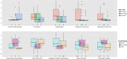
Figure 2 The most explanatory variables for post-disturbance watershed response, with predictor variables shown as standardized anomalies, e.g. subtracted the mean then divided by the standard deviation, and binned into response groups. Therefore the y-axis shows the number of standard deviations from the mean computed for all watersheds (e.g. across all groups) for each variable. Differences among groups illustrate their associative values relative to watershed response in terms of water yield (top) or streamflow timing (bottom). For example, large values of percent forest disturbed were strongly associated with observed increases in water yield. High snow percentage was associated with insensitivity to disturbances in terms of streamflow timing. Soil <2 mm refers to the fine fraction percentage of the total soil volume. Numbers indicate significantly different groups (p < 0.05, pairwise Kruskal–Wallis rank sum test). Boxplots show 25th and 75th percentiles, whiskers extent to 1.5 the interquartile range beyond those percentiles. Outliers are shown as points.
Download figure:
Standard image High-resolution image3.1. Water yield change
Disturbance from a combination of natural and anthropogenic sources was the most important variable in predicting post-disturbance yield change, with larger disturbances associated with increased runoff (p < 0.01). Cumulatively, watersheds with increased water yield had a significantly higher (p < 0.01) percent of their forested area disturbed (group mean 47%, median 15%) compared to those with decreased water yield (mean 16%, median 9%) or did not change (mean 10%, median 9%). Watersheds with persistent disturbances, measured as cumulative (multi-year) area disturbed prior to the major disturbance year, were more sensitive to a large disturbance event in a single year than those without persistent disturbances.
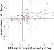
The trend in water yield change was also compared to the percent of the watershed disturbed without grouping watersheds. Disturbances greater than > 7% of the forested area were associated with increased water yield, while disturbances greater than > 20% showed even greater increases (p < 0.05; figure 3). This is consistent with previous studies associating streamflow increases with disturbance, but also with the notion of a minimum disturbance threshold for detecting hydrologic response [Brown et al 2005, Bosch and Hewlett 1982, Stednick 1996]. Interestingly, a disturbance threshold of 20% disturbed area was previously proposed [Stednick 1996] as the minimum for detecting yield changes (typically increasing) in forested watersheds, though recent, more fine-scaled work has found responses at smaller harvest areas [e.g. Hornbeck et al 1997] and others have suggested that watershed size plays a role in the disturbance area-streamflow response relationship, with smaller headwater watersheds likely less sensitive than the larger watersheds [Trimble et al 1987]. Our findings demonstrate that observable hydrologic responses can be detected for smaller disturbance extents (<20%) at multiple watershed sizes.
Figure 3 Absolute water yield change as a function of total loss area. All undammed watersheds which experienced >1% disturbance are shown (n = 73). The normalized yield response refers to the change in runoff ratio post-disturbance after controlling for precipitation inputs, i.e. the detrended runoff ratio residual (dRRR); positive values indicate increased water yield. The horizontal line at y = 0 indicates no change. The trend line is significant (p < 0.05, linear regression), indicating that water yield increases with increasing disturbance extent. The dashed vertical line is at 20% disturbed. The solid vertical line indicates the point where responses generally trend positive, at approximately 7% of total area disturbed (log(0.07) = −2.66).
Download figure:
Standard image High-resolution image
Watersheds where dRRR was highly positive, meaning more runoff than expected after accounting for precipitation, had generally higher percentage of area disturbed, lower precipitation, lower fragmentation, and lower deciduous forest cover (and thus higher coniferous and mixed forest cover), and lower subsurface contact time, a measure of the residence time (days) of water in the saturated subsurface zone of the watershed [Falcone et al 2010, figure 2]. Average soil bulk density (g cm−3) was also significantly higher in watersheds with increased RR post-disturbance compared to insensitive or declining RR watersheds, as was permeability (though not significantly so).
Insensitive watersheds generally exhibited intermediate values of the explanatory variables relative to those watersheds that increased or decreased their yields. This intermediate relationship was true for all the top five variables identified (figure 2). For example, median precipitation was highest in watersheds that decreased their water yield post-disturbance, and was sequentially higher in the no-change, and decreasing groups, respectively.
Interestingly, wet regions (high precipitation) were generally associated with a lower RR than expected post-disturbance (figure 2). We hypothesize that this occurs when rapid (within a year of disturbance, and thus included in our methods) understory regrowth/rapid recovery of post-disturbance vegetation (such as the filling of small, gap openings by neighboring trees) compensates for canopy loss [Helvey and Tiedemann 1978, Runkle 1982, Buchanan and Hart 2012] as biological structures, e.g. leaves, are rebuilt [Trimble et al 1987, Hornbeck et al 1997, Fernandez et al 2006, Brookhouse et al 2013]. We note that high fractions of deciduous cover (often re-sprouting species) and longer contact time between water and soil, and thus plant available water, are strong predictors for water yield reduction post-disturbance, similar to previous work [Voepel et al 2011, Jasechko et al 2013, Brantley et al 2014]. This outcome is also in partial agreement with previous research which found that clear-cut deciduous and grassland dominated watersheds typically show smaller increases in water yield compared to coniferous forests [Sahin and Hall 1996, Bosch and Hewlett 1982].
3.2. Streamflow timing change
There was a significant relationship between streamflow timing change and water yield change, with earlier streamflow associated with increases in water yield (chi-squared test, p < 0.05, figure S3). Earlier streamflow timing was also associated with greater percent of the watershed disturbed (mean percent disturbed 8.6%, median 2.7%) relative to no change (mean 6.9%, median 2.6%) and later timing (mean 5.7%, median 2.0%). In contrast to water yield, the strongest contrast was between insensitive and sensitive watersheds, not between the sign of response of the sensitive groups (figure 2, bottom row). Insensitive watersheds generally had a higher percentage of snow, lower percentage of fine soils, and steeper slopes. We hypothesize that the insensitivity seen here is a result of temporally dependent factors driving streamflow timing (e.g. yearly weather driving early or late snowmelt) rather than disturbance characteristics. The lack of distinguishing characteristics among sensitive watersheds (e.g. earlier vs. later) was surprising, and suggests that the relevant drivers are not static watershed features, like slope. Disturbance characteristics are potential explanations, for example fire can dramatically alter runoff rates by increasing hydrophobicity [Wondzell and King 2003], whereas insect mortality does not have, nor is expected to have, the same effect [Helvey and Tiedemann 1978, Pugh and Gordon 2013]. Vegetation composition is also likely important; watersheds with extensive shrublands showed later streamflow timing (mean 25.5% shrubland) relative to the insensitive and earlier streamflow groups (19.3% and 16.1% shrubland, respectively). This research did not focus on multi-year forest recovery and was only interested in hydrological response in the year following disturbance. Overall the finding of later streamflow timing in watersheds with high shrubland coverage is consistent with research suggesting delayed streamflow timing is driven by understory and shrub regeneration [Johnson and Kovner 1956, Fernandez et al 2006, Guardiola-Claramonte et al 2011].
4. Conclusions
Vegetation is an important mediator of water movement into and out of catchments multiple scales [Thompson et al 2011] and as a result, vegetation disturbance can cause substantial water balance variability. Previous research looking for broad scale patterns frequently used indices as a means to predict hydrological response to vegetation disturbance. For example, reductions in catchment vapor, i.e. ET, loss as it relates to the watershed Horton Index (ratio of total vapor losses to plant-available water) and partitioning flow into fast and slow components were identified as useful predictors of watershed response [Voepel et al 2011, Harman et al 2011]. Here we take a different, but complimentary approach by utilizing extensive spatial information on soils, climate, and anthropogenic activities and statistical associations to further refine our understanding of vegetation change and streamflow response. Although regional precipitation trends likely exist during the study period, the detrending of response variables (dRRR and timing) by observed precipitation minimizes the influence of any regional climatic trends over that time. Water yield changes are observable despite the fact that our analysis did not differentiate between disturbance type (fire, insect mortality, harvest, etc.). This stands as a limitation of currently available highly validated remote sensing products. Management treatments, such as clear cutting vs. partial harvest, can be designed to alter water yield intentionally [Douglass 1983], and different anthropogenic disturbances influence hydrology in unique ways [Hornbeck et al 1997]. This study did not distinguish those treatments with other forms of disturbance. In some cases, specific disturbance processes may result in differing effects, such as forest declines; a recent review suggested that low precipitation, rain dominated watersheds were more likely to experience no change or decreased streamflow [Adams et al 2012]. The work presented here also did not consider potential land use changes post-disturbance, such as appropriating forests for agriculture. Despite these limitations, and the resultant unaccounted for variability in observed response, predictable patterns were seen at the national level. Future work should incorporate longer historical time horizons, using paleo reconstructions of disturbance events and subsequent water proxy responses (e.g. tree ring methodologies) to determine historical variability.
At this broad scale, which spans multiple climate contexts, topographic and soil settings, and disturbance processes, we suggest the link between water yield and streamflow timing immediately post-disturbance, at the study scale, can be primarily attributed to soil conditions and disturbance extent. First, the residence time of water in the soil was shown to be critical: Longer soil contact time/slower drainage [Wolock et al 1989, Wolock 1997] makes water more readily available for ET losses. This outcome corresponds to another broad-scale analysis by Voepel et al [2011] which found that steeper slopes correspond with decreases in relative vaporization by vegetation. Lower residence times in the soil would serve to increase the likelihood of increased streamflow post-disturbance because a lower fraction of water is interacting with vegetation pre-disturbance. Using a larger subset of the same dataset, Harman et al [2011] similarly found the fraction of water in the surface soil layers (fast component) varied more rapidly than deeper moisture in response to yearly climate, partially mediated through changes in vegetation activity and associated ET controls. While Voepel et al [2011] utilized topography as a proxy for partitioning water into plant-available and subsurface fractions, here we found a stronger relationship to subsurface contact time, a more integrated variable that includes both soil information and topography [Wolock 1997]. This characteristic is generally considered static across time, dependent on soil and topography (figure S4), however we acknowledge that soil properties can be altered by disturbance e.g. post-fire soil hydrophobicity decreases contact time.
Second, disturbance extent was shown to strongly influence water yield, with a significant but small effect on streamflow timing. Increasing water yield with increasing disturbance extent supports the idea that transpiration reductions are the primary driver of water yield change post-disturbance (e.g. Johnson and Kovner 1956). Yet, rapid recovery of hydrological functioning has been observed in several systems [Guardiola-Claramonte et al 2011, Brantley et al 2014, Brookhouse et al 2013] and is likely favored by low severity disturbance events. For example, forests recover quickly (e.g. over the subsequent growing season) from many non-lethal defoliators, rapidly rebuilding water intensive structures. Recovery from wildfires can similarly be enough to partially mitigate hydrological impacts [Hallema et al 2016]. As a result, impacts to water supplies are typically minor and only observed in extreme years [Helvey and Tiedemann 1978]. This recovery pathway stands in contrast to lethal insect outbreaks, from which forests and forest hydrology may take decades to recover [Pugh and Gordon 2013]. The results presented here highlight how local contexts constrain and influence any disturbance effects on immediate hydrological properties, and should be interpreted at the scale of individual watersheds by local research and expert knowledge.
A novel feature of this work is the implementation of a broad set of mechanistic variables (e.g. soil-water contact time) and an extremely wide range of disturbance severities over a large number of watersheds. As the regional distribution of precipitation changes due to shifting climates, areas of relative water scarcity and surplus will be further modulated by forest dynamics. Understanding the sensitivity of water-supplying landscapes to forest disturbance will become increasingly important. Some of the characteristics identified here may themselves respond to climate change, such as shifting forest composition and snow fractions. Future efforts to integrate plot-scale theory and in situ observations together with emerging national-scale disturbance datasets will help to refine predictions of watershed-disturbance responses.
Acknowledgments
This work was partially supported by Alaska EPSCoR NSF award #OIA-1208927. Publication of this article was funded by the University of Colorado Boulder Libraries Open Access Fund. Supporting data, intermediate results, and all final coefficients can be found in the supplementary data. R code is available from the authors. We thank Paul Brooks and two anonymous reviewers for constructive comments on previous versions of the manuscript.