


ABSTRACT
We present Keck/DEIMOS spectroscopy and Canada–France–Hawaii Telescope/MegaCam photometry for the Milky Way globular cluster Palomar 13. We triple the number of spectroscopically confirmed members, including many repeat velocity measurements. Palomar 13 is the only known globular cluster with possible evidence for dark matter, based on a Keck/High Resolution Echelle Spectrometer 21 star velocity dispersion of σ = 2.2 ± 0.4 km s−1. We reproduce this measurement, but demonstrate that it is inflated by unresolved binary stars. For our sample of 61 stars, the velocity dispersion is σ = 0.7+0.6−0.5 km s−1. Combining our DEIMOS data with literature values, our final velocity dispersion is σ = 0.4+0.4−0.3 km s−1. We determine a spectroscopic metallicity of [Fe/H] = −1.6 ± 0.1 dex, placing a 1σ upper limit of σ[Fe/H] ∼ 0.2 dex on any internal metallicity spread. We determine Palomar 13's total luminosity to be MV = −2.8 ± 0.4, making it among the least luminous known globular clusters. The photometric isophotes are regular out to the half-light radius and mildly irregular outside this radius. The outer surface brightness profile slope is shallower than typical globular clusters (Σ∝rη, η = −2.8 ± 0.3). Thus at large radius, tidal debris is likely affecting the appearance of Palomar 13. Combining our luminosity with the intrinsic velocity dispersion, we find a dynamical mass of M1/2 = 1.3+2: 7−1.3 × 10³M☉ and a mass-to-light ratio of M/LV = 2.4+5.0−2.4M☉/L☉. Within our measurement errors, the mass-to-light ratio agrees with the theoretical predictions for a single stellar population. We conclude that, while there is some evidence for tidal stripping at large radius, the dynamical mass of Palomar 13 is consistent with its stellar mass and neither significant dark matter, nor extreme tidal heating, is required to explain the cluster dynamics.
Export citation and abstract BibTeX RIS
1. INTRODUCTION
Globular clusters are among the oldest structures in the universe. Current models favor globular cluster formation via the collapse of cold gas within a larger galactic environment (Fall & Rees 1985; Kravtsov & Gnedin 2005; Muratov & Gnedin 2010). Recently, improved evidence for internal abundance ratios of elements heavier than hydrogen in some of the most luminous globular clusters (e.g., Lee et al. 2009; Cohen et al. 2010; Milone et al. 2011) has renewed interest in the idea that these objects might instead have formed at the center of their own dark matter halos (Peebles 1984) or are the stripped nuclei of dwarf galaxies (Bekki & Freeman 2003), thus providing a deeper gravitational potential for the retention of enriched material. Observational evidence, however, argues against dark matter in globular clusters, at least at the present time. Photometric studies of cluster profiles (Conroy et al. 2010) and dynamical studies of Milky Way globular clusters (Baumgardt et al. 2009; Lane et al. 2010; Hankey & Cole 2011) show no evidence for dark matter, at least out to the tidal radius in these systems.
An interesting possible exception to the conclusion that globular clusters do not contain dark matter is Palomar 13 (Pal 13), a low-luminosity Milky Way globular cluster (MV ∼ −3.7; Harris 2010) at a Galactocentric distance of 25 kpc. The combined size and luminosity of Pal 13 (see Figure 1) is more similar to the Milky Way ultra-faint galaxies than a typical Milky Way globular cluster (Martin et al. 2008). Motivated in part by its low luminosity and relatively large size, Côté et al. (2002, hereafter C02) measured velocities for 21 member stars in Pal 13 based on Keck/High Resolution Echelle Spectrometer (HIRES) spectroscopy. Their velocity dispersion of 2.2 ± 0.4 km s−1 is well in excess of that predicted from the stellar mass of Pal 13 alone. In contrast, velocity dispersions of six other extended outer halo globular clusters measured by these authors are consistent with their stellar masses (Baumgardt et al. 2009). C02 also measure a shallow surface brightness profile for Pal 13 and a King tidal radius that is significantly larger than the predicted tidal radius based on the stellar mass of the cluster. C02 interpreted the inflated velocity dispersion and shallow luminosity density profile of Pal 13 as due either to tidal heating during a recent perigalacticon passage, implying that the cluster is not in dynamical equilibrium, or the presence of dark matter. If Pal 13 is in dynamical equilibrium, its measured velocity dispersion implies the highest mass-to-light ratio known in a globular cluster, M/LV = 40+24−17 M☉/L☉.

Figure 1. Absolute magnitude vs. half-light radius for all Milky Way globular clusters (blue triangles, data from Harris 2010), dSphs (green circles), and ultra-faint galaxies (red circles). The open triangle represents Pal 13 based on literature values, the blue star is the position of Pal 13 based on quantities we determine based on deeper CFHT/MegaCam photometry.
Download figure:
Standard image High-resolution imageThe proper motion of Pal 13, measured by Siegel et al. (2001) via photographic plates, implies that this cluster is on a highly eccentric orbit near perigalacticon. This is consistent with the interpretation that Pal 13 is in the final stages of tidal disruption, and its increased velocity dispersion is due to tidal heating. However, N-body simulations by Küpper et al. (2011) are unable to reproduce either the inflated velocity dispersion or shallow density profile using the measured orbit. Interestingly, these authors can reproduce the photometric properties of Pal 13 assuming that instead it is near apogalacticon, i.e., at the farthest point in its orbit. In this case, the observed surface brightness profile is not due to tidal heating, but rather due to projection effects as unbound stars, removed in the course of slow tidal evaporation, are compressed near apogalacticon. In these simulations, binaries are still required to explain the observed velocity dispersion.
A high unresolved binary star fraction is a third proposed explanation for the large velocity dispersion observed in Pal 13. Clark et al. (2004) estimated the Pal 13 binary star fraction as 30% ± 4% based on a secondary red main sequence and the presence of a large number of blue straggler stars (BSSs). This is higher than observed for more massive globular clusters, but consistent with that of lower mass globular clusters. Blecha et al. (2004) measured a lower velocity dispersion (0.6–0.9 ± 0.3 km s−1) for Pal 13 based on eight member stars. Seven of these stars overlap with C02 (note Blecha et al. state only six), including three stars which are identified as velocity variables in one or both samples. Given the small number of stars, it is yet unclear whether binaries can indeed provide an explanation for the high velocity dispersion in Pal 13 without invoking tidal heating or the presence of dark matter.
Here we present Keck/DEIMOS spectroscopy and Canada–France–Hawaii Telescope (CFHT)/MegaCam imaging of the Milky Way globular cluster Pal 13. The paper is organized as follows: in Section 2 we discuss data acquisition and reduction for both our spectroscopic and photometric data sets, including estimates of structural parameters. In Section 3, we discuss the techniques used to identify spectroscopic members. In Section 4, we determine the velocity dispersion, mass and mass-to-light ratio of Pal 13, and compare to previous results. In Section 4, we also examine the blue straggler population of Pal 13. Finally, in Section 5 we interpret our results, concluding that the kinematics of Pal 13 are consistent with its stellar mass and find only mild evidence for tidal effects at large radii.
Throughout this paper, we adopt a distance to Pal 13 of 24.3 kpc (RGC = 25.3 kpc; Côté et al. 2002) and reddening of E(B − V) = 0.11 (Schlegel et al. 1998). These values are in good agreement with our own isochrone fitting of the photometry described in Section 2.2.1.
2. DATA ANALYSIS
2.1. Spectroscopic Targeting
We select spectroscopic targets in Pal 13 based on CFHT CFH12K and Keck/Low Resolution Imaging Spectrometer (LRIS) imaging as described in C02. We supplement these data at large radius with wider field photometry from P. Stetson's online database.7 Candidate Pal 13 member stars were identified in V- and I-bands, and V- and R-band when I-band was not available. This isochrone was used for target selection only; a slightly better fitting isochrone is used in the subsequent analysis (see Figure 2). Targets were selected based on proximity to a Girardi et al. (2002) theoretical isochrone for an age of 12 Gyr and a metallicity of [Fe/H] =−1.7 (Zinn & Diaz 1982; Friel et al. 1982; Côté et al. 2002). This isochrone was used for target selection only; a slightly better fitting isochrone is used in the subsequent analysis. We determine a star's distance to the isochrone via the quantity ![$d = \sqrt{[(V-I)_* - (V-I)_{\rm iso}]^2 + (V_* -V_{\rm iso})^2}$](https://content.cld.iop.org/journals/0004-637X/743/2/167/revision1/apj409888ieqn1.gif) . Stars on the red giant branch (V ⩽ 20.5) within d = 0.1 mag of the isochrone were given the highest priority for spectroscopy; stars within 0.2 mag of the isochrone were given lower priority. On the subgiant branch and main sequence (V > 20.5) and on the horizontal branch the selection region was widened to within 0.2 and 0.3 mag of the isochrone for the higher and lower priority categories, respectively. Candidate BSSs were chosen in a box blueward of and brighter than the main-sequence turnoff/subgiant branch region. Following the photometric selection, spectroscopic targeting priorities were set to favor known radial-velocity members from C02 and Blecha et al. (2004), and likely proper motion members from Siegel et al. (2001).
. Stars on the red giant branch (V ⩽ 20.5) within d = 0.1 mag of the isochrone were given the highest priority for spectroscopy; stars within 0.2 mag of the isochrone were given lower priority. On the subgiant branch and main sequence (V > 20.5) and on the horizontal branch the selection region was widened to within 0.2 and 0.3 mag of the isochrone for the higher and lower priority categories, respectively. Candidate BSSs were chosen in a box blueward of and brighter than the main-sequence turnoff/subgiant branch region. Following the photometric selection, spectroscopic targeting priorities were set to favor known radial-velocity members from C02 and Blecha et al. (2004), and likely proper motion members from Siegel et al. (2001).

Figure 2. CMD for CFHT photometric data within 5' of Pal 13's center. Several Girardi et al. (2002) isochrones are plotted with [Fe/H] =−1.6 dex for various ages shown in the legend.
Download figure:
Standard image High-resolution image2.2. Spectroscopic Observations and Data Reduction
The spectroscopic data were taken with the Keck II 10 m telescope and the DEIMOS spectrograph (Faber et al. 2003). Eight multislit masks were observed in Pal 13 in 2008 September, with a ninth mask obtained in 2009 October. Exposure times, observation dates, and other observing details are given in Table 1. The masks were observed with the 1200 line mm−1 grating covering a wavelength region 6400–9100 Å. The spectral dispersion of this setup was 0.33 Å pixel−1, equivalent to R = 6000 for our 0 7 wide slitlets, or an FWHM of 1.37 Å. The spatial scale was 012 pixel−1. The minimum slit length was 5'' which allows adequate sky subtraction; the minimum spatial separation between slit ends was 04 (3 pixels).
Table 1. Keck/DEIMOS Multislit Mask Observing Parameters
| Mask | α (J2000) | δ (J2000) | Date Observed | P.A. | texp | No. of Slits | % Useful |
|---|---|---|---|---|---|---|---|
| Name | (h:m:s) | (°: ': '') | (deg) | (s) | Spectra | ||
| Pal13_1 | 23:07:03.4 | +12:50:55 | 2008 Sep 4 | 38 | 9000 | 74 | 86% |
| Pal13_2 | 23:06:50.8 | +12:49:09 | 2008 Sep 4 | −13 | 7200 | 81 | 95% |
| Pal13_3 | 23:06:47.3 | +12:44:14 | 2008 Sep 5 | 112 | 7200 | 72 | 94% |
| Pal13_4 | 23:06:41.7 | +12:43:45 | 2008 Sep 5 | 180 | 8100 | 83 | 95% |
| Pal13_5 | 23:06:08.4 | +12:49:16 | 2008 Sep 4 | 17 | 2700 | 52 | 96% |
| Pal13_6 | 23:07:22.7 | +12:49:25 | 2008 Sep 4 | −166 | 2460 | 56 | 98% |
| Pal13_7 | 23:06:31.2 | +12:37:44 | 2008 Sep 5 | 87 | 2400 | 51 | 92% |
| Pal13_8 | 23:06:42.3 | +12:45:54 | 2008 Sep 5 | 74 | 1680 | 42 | 83% |
| pal13 | 23:06:51.0 | +12:45:14 | 2009 Oct 13 | 0 | 1800 | 23 | 96% |
Notes. The right ascension, declination, date of observation, position angle, and total exposure time for each Keck/DEIMOS slitmask. The final two columns refer to the total number of slitlets on each mask and the percentage of those slitlets for which a redshift was measured.
Download table as: ASCIITypeset image
Spectra were reduced using a modified version of the spec2d software pipeline (version 1.1.4) developed by the DEEP2 team at the University of California-Berkeley for that survey. A detailed description of the reductions can be found in Simon & Geha (2007). The final one-dimensional spectra were rebinned into logarithmic wavelength bins with 15 km s−1 pixel−1. Radial velocities were measured by cross-correlating the observed science spectra with a series of high signal-to-noise stellar templates. We employ the telluric absorption lines in the stellar spectra to calculate and apply a correction for the radial-velocity errors that arise from a miscentering of the star in the spectrograph slit. Each science spectrum is cross-correlated with a hot stellar template where the telluric absorption lines are the dominant spectral features. Since these lines are illuminated by the stellar flux, this defines the star's photocenter within the slit in velocity space. We applied both a telluric and heliocentric correction to all velocities presented in this paper.
We determined the random component of our velocity errors using a Monte Carlo bootstrap method. Noise was added to each pixel in the one-dimensional science spectrum, we then recalculated the velocity and telluric correction for 1000 noise realizations. Error bars are defined as the square root of the variance in the recovered mean velocity in the Monte Carlo simulations. The systematic contribution to the velocity error was determined by Simon & Geha (2007) to be 2.2 km s−1 based on repeated independent measurements of individual stars and we refer the reader to this paper for further details. The systematic error contribution is expected to be constant as the spectrograph setup and velocity cross-correlation routines are identical. We added the random and systematic errors in quadrature to arrive at the final velocity error for each science measurement. Radial velocities were successfully measured for 482 of the 566 extracted spectra across the nine observed DEIMOS masks. The fitted velocities were visually inspected to ensure reliability. We identified 90 sources as background galaxies or QSOs and obtained repeat measurements for 62 stellar sources. Our final stellar sample consists of 392 measurements of 306 unique stars.
2.2.1. Deep CFHT MegaCam Imaging of Palomar 13
After our spectroscopic observations, we obtained significantly deeper images of Pal 13 using the CFHT MegaCam imager. These images were taken as part of a larger program aimed at obtaining deep wide-field imaging of all bound stellar overdensities in the Galactic halo beyond 25 kpc (R. Muñoz et al. 2011, in preparation). Pal 13 was observed on the night of UT 2009 July 22 under dark conditions with typical seeing of 07–09. We obtained six dithered exposures of 360 s in both the g- and r-bands centered on Pal 13. A standard dithering pattern was used to cover both the small and large gaps present between chips.
Data from MegaCam were pre-processed prior to release using the "ELIXIR" package (Magnier & Cuillandre 2004). This pre-process includes bad pixel masking, bias subtraction, flat fielding as well as preliminary photometric and astrometric solutions. We carried out subsequent data reduction following the method detailed in Muñoz et al. (2010) which relies on the DAOPHOT/Allstar/ALLFRAME packages (Stetson 1994). To refine the astrometric solutions included in the image headers, we have used the SCAMP package (Bertin 2006) using as reference the USNO-B1 catalog, which yielded astrometric residuals of rms ∼ 04.
Photometric calibration is achieved by comparing directly to Pal 13 data from the Sloan Digital Sky Survey (SDSS) Data Release 8 (DR8; Aihara et al. 2011). To determine zero points and color terms we used stars with magnitudes in the range 18 < r < 21 and −0.25 < g − r < 1.0, providing 2950 matches between our catalog and SDSS. Final solutions for the zero points and color terms yield uncertainties of ∼0.004 mag and ∼0.007 mag, respectively, for both passbands. Our photometric catalog reaches 90% completeness at r ∼ 24.1.
2.2.2. Improved Structural Parameters for Palomar 13
Using our CFHT/MegaCam catalog, we recalculated structural parameters for Pal 13 using a Maximum Likelihood method as described in Muñoz et al. (2010). In this method, a fixed analytic profile is assumed and its free parameters are fit using all the available stars in the color-magnitude diagram (CMD) selection window. This avoids the need to bin or smooth data, providing more reliable estimates for systems with low numbers of stars (Martin et al. 2008). We simultaneously estimated the scale length, the central coordinates, the ellipticity, the position angle, and the background density of Pal 13. We assumed an empirical King profile (King 1962), for which we calculated a King core (rc) and tidal (rt) radius. We additionally fit a Navarro–Frenk–White (NFW; Navarro et al. 1997) and a Plummer profile (Plummer 1911), a good representation for dwarf galaxies, but found that these were poor fits to the light distribution shape of Pal 13. The best-fitting King parameters are rc = 0 42 ± 006 (3.0 ± 0.4 pc) and rt = 139 ± 15 (98 ± 11 pc). The two-dimensional half-light radius of this King profile is r1/2 = 127 ± 016 (9.0 ± 1.1 pc). The overall ellipticity of Pal 13 is consistent with being zero and therefore its position angle is poorly constrained.
In the left panel of Figure 3, we show the projected density profile for Pal 13, overplotting our best-fit King profile. Error bars on the data points include uncertainty in determining the background level which dominates outside r ∼ 7'. We emphasize that the King profile shown is not a direct fit to the data points, but constructed with the best-fit parameters obtained through the maximum likelihood estimator. We compared our best-fitting King profile to that determined in C02. If we parameterize the outer slope of the surface brightness profile as Σ∝r−η, then typical globular clusters have slopes of η ∼ 4 (McLaughlin & van der Marel 2005). We measure a shallow slope for Pal 13 of η = 2.8 ± 0.3. This is consistent with our inferred King tidal radius which is two times larger than the calculated tidal radius of Pal 13 based on its stellar mass and distance from the Milky Way (see Section 3). Our inferred slope is steeper than the C02 estimate of η = 1.8 ± 0.2. These two profiles are compared in Figure 3. A key difference between the two King profiles is the CMD region in which they were determined. While C02 determined the profile using stars inside a box in CMD space, we have used a window around the best-fitting isochrone. At faint magnitudes, there is significant contamination from unresolved galaxies, and our CMD window should reduce this contamination.

Figure 3. Left: Pal 13 surface brightness profile based on CFHT/MegaCam imaging reaching a magnitude limit of r = 24. Here we compare our best-fitting King profile (solid) to that from C02 (dotted) and parameterize the outer slope of the surface brightness profile (dashed). The dot-dashed line represents the background level. Right: the surface density profile for Pal 13. The outermost contours are our 3σ confidence limits, corresponding to 30 mag arcsec−2. The dashed red line in both panels is plotted at the King tidal radius of rt = 139 = 98 pc.
Download figure:
Standard image High-resolution imageIn the right panel of Figure 3, we show the spatial density map of Pal 13. The outer isophotes in this figure are 3σ contours above the background, corresponding to r ∼30 mag arcsec−2. The red dashed line/circle in both panels of Figure 3 are drawn at the King tidal radius rt = 139 (98 pc). The photometric isophotes are regular out to the half-light radius of the cluster and appear mildly irregular outside this radius. This is in contrast to other faint globular clusters such as Palomar 1 and Palomar 5 which show evidence for tidal tails at much brighter surface brightness levels (Niederste-Ostholt et al. 2010; Odenkirchen et al. 2003), although similar to that observed for Palomar 14 (Sollima et al. 2011). We interpret the slightly irregular isophotes and shallow density profile as mild evidence for tidal disruption and discuss further in Section 5.
Finally, we estimated the total luminosity of Pal 13. The published values for Pal 13 range between 1.2 × 10³ and 3.5 × 10³ L☉ (Siegel et al. 2001; Côté et al. 2002), making traditional methods of adding stars' individual fluxes too sensitive to the inclusion (or exclusion) of potential members (outliers). To alleviate these shot noise issues, the method used here relies solely on the total number of stars belonging to the satellite and not on their individual magnitudes (Muñoz et al. 2010). To estimate an absolute magnitude, we modeled the satellite's population with the best-fitting theoretical luminosity function, in this case a 12 Gyr population with [Fe/H]=−1.6 (Girardi et al. 2002). We then integrated the theoretical luminosity function to obtain the total flux down to a given magnitude limit. The last step was to scale this flux using the total number of Pal 13 stars in our catalog down to the same magnitude limit. To estimate the uncertainty in the absolute magnitude we carried out a bootstrap analysis generating 10,000 realizations of Pal 13 from the photometric data (for more details see Muñoz et al. 2010). We assumed a Chabrier initial mass function for the estimation (Bruzual & Charlot 2003). We obtained MV = −2.8 ± 0.4, or equivalently LV = 1.1+0.5−0.3 × 10³ L☉. The central surface brightness is μ0, V = 23.9+0.6−0.7 mag arcs−2. While our results are 1σ lower than published values, it is a more robust estimate of the true luminosity of Pal 13 as it better accounts for shot noise in this quantity. We list our measured properties of Pal 13 and those of C02 in Table 2 for comparison.
Table 2. Palomar 13 Properties
| Property | Côté et al. (2002) | This Work |
|---|---|---|
| Core radius (King model), rc | 0.23 ± 0.03 arcmin | 0.42 ± 0.06 arcmin |
| Tidal radius (King model), rt | 26 ± 6 arcmin | 13.9 ± 1.50 arcmin |
| Half-light radius (King model), r1/2 | N/A | 1.27 ± 0.16 arcmin |
| Luminosity, LV | (2.8 ± 0.4) × 103 L☉ | (1.1+0.5−0.3) × 103 L☉ |
| Absolute magnitude, MV | −3.8 mag | −2.8 ± 0.4 mag |
Metallicity, ![$\rm [Fe / \rm H]$](https://content.cld.iop.org/journals/0004-637X/743/2/167/revision1/apj409888ieqn2.gif) |
−1.9 ± 0.2 dex | −1.6 ± 0.1 dex |
| Right ascension (center, King model), R.A. | 346 6867 6867 |
34668519 ± 000063 |
| Declination (center, King model), decl. | 127717 |
12771539 ± 000068 |
| Distance modulus, (m − M)0 | 16.93 ± 0.10 mag | N/A |
| Distance, d | 24.3+1.2−1.1 kpc | N/A |
Notes. We list properties of Pal 13 compiled by C02 and as independently measured by this work for comparison.
Download table as: ASCIITypeset image
3. MEMBERSHIP CRITERIA
The systemic velocity of Pal 13 lies within the velocity distribution of foreground Milky Way stars. We therefore selected spectroscopic members of Pal 13 by combining color–magnitude and velocity criteria with proper motion information from the literature.
We first applied a color–magnitude selection window shown in Figure 4. CMD selection was performed using a 12 Gyr, [Fe/H] = −1.6 Girardi et al. (2002) isochrone in the CFHT photometric system, shown in Figure 2 to fit Pal 13. The selection window was defined as 0.1 mag around this isochrone added in quadrature to the 2σ photometric errors. The CMD selection window does not include BSSs which are abundant in Pal 13 (Clark et al. 2004). We selected blue stragglers separately by defining a generous window bluer and brighter than the main-sequence turnoff, but dimmer than the horizontal branch (Figure 4). Stars in the blue straggler window are removed from all analysis below unless specified. We study the blue straggler population separately in Section 4.5.

Figure 4. Left: CMD of Pal 13 based on CFHT imaging for all spectroscopic stellar targets. The primary color selection window is plotted in light red with the best-fitting isochrone centered as a black dotted line. The blue straggler selection window is plotted in light blue. Red circles represent likely velocity members within the primary selection window, red squares in this region are further confirmed as Pal 13 members via proper motions. Small black dots represent definite non-members. We also identify two stars from the C02 study as orange stars. ORS-91 lies near the horizontal branch and ORS-38 lies near the red giant branch (RGB). Right: spatial diagram of Pal 13 for all spectroscopic stellar targets. Symbols are the same as the CMD plot on left. The solid circle is the cluster's half-light radius (r1/2 = 09). The dashed red circle represents the King tidal radius (rt = 139).
Download figure:
Standard image High-resolution imageAfter the CMD selection, we applied a basic velocity cut to the sample. We chose a conservative velocity window of 10σ around the systemic velocity as measured by C02. We use the velocity dispersion measured by C02 of σ = 2.2 km s−1, thus our velocity window corresponds to ±22 km s−1 around the systemic velocity of 26.2 km s−1. Combined with stars passing the CMD cut, this leaves 93 member candidates of Pal 13.
Milky Way foreground stars are expected to contaminate our CMD and velocity selected sample. Using the Besançon model of the Milky Way (Robin et al. 2003), we applied the same selection criteria and predict 5–7 foreground stars in our sample of 93 Pal 13 members, depending on details of normalizing the model to data. A maximum of six of these possible seven foreground stars are predicted in the thin and thick disk, and one in the halo. A method to identify foreground stars is via metallicity, since the average [Fe/H] of Pal 13 is significantly lower than expected for the majority of foreground Milky Way disk stars (Section 4.4). As explained in Section 4.4, we can measure metallicities for only the 20 brightest stars in our sample. As seen in Figure 7, four stars are far more metal-rich compared to the main sample. Three stars are at very large radius from Pal 13 where the contamination is greatest. We reject these four stars as members, leaving 89 candidate Pal 13 stars in our "full" sample.
Another way to identify foreground stars is via proper motions. Proper motions are available for 69 out of 89 candidate members (78%) from Siegel et al. (2001). Three stars in this sample have large proper motions that are inconsistent with being cluster members (assigned 0% membership probabilities by Siegel et al.), and we eliminate them from our sample. This leaves 66 candidate member stars of Pal 13. We defined this sample of 66 stars as our "cleaned" Pal 13 sample and proceed with analysis on these stars. We cannot be certain the cleaned sample is free of Milky Way contamination, but estimate from the Besançon models that there is likely less than one foreground star given our sample criteria. The results of this selection are shown in Figure 5.

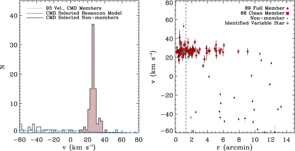
Figure 5. Left: velocity histogram of Pal 13 stars passing our primary color–magnitude selection criterion. We use a bin size of 2.5 km s−1 representing the typical velocity error. The normalized Milky Way model is plotted as a solid blue line and estimates the foreground contamination in each bin. CMD-selected non-members are plotted as a solid black line and exclude blue stragglers. Right: velocity of CMD-selected stars as a function of cluster radius. The dashed line represents the half-light radius. Red circles represent CMD and velocity selected Pal 13 stars, red squares are stars which are further confirmed as Pal 13 members via proper motions. Small black dots show non-members. We also identify binaries as blue diamonds.
Download figure:
Standard image High-resolution imageTidal heating or evaporation processes will unbind stars from the gravitational potential of Pal 13. These stars can be a source of contamination if they remain in the spatial vicinity of the cluster and would not be rejected by our methods above (Klimentowski et al. 2007). While the three stars at largest radius passing our CMD and velocity cuts are prime candidates for unbound Pal 13 stars, these were rejected based on their high metallicity and are more likely to be Milky Way foreground stars.
To estimate at what projected radius stars are likely to be unbound from Pal 13, we calculate the Jacobi tidal radius assuming a Galactocentric distance of 25.3 kpc and a Milky Way mass inside this radius of 3 × 10¹¹ M☉. The Jacobi tidal radius of Pal 13 is 67 (47 pc), larger than the half-light radius of the cluster reff = 13, but smaller than the inferred King tidal radius of rt = 139, as noted previously by C02, Siegel et al. (2001), and Küpper et al. (2011). Although the Jacobi radius provides only a very approximate estimate of the tidal radius (Binney & Tremaine 2008), this suggests that stars in the outskirts of Pal 13 may not be bound to the cluster. This calculation assumes a circular orbit. Stars in our "clean" kinematic sample are located well inside the Jacobi tidal radius, while our full sample contains two stars beyond this distance.
3.1. Repeated Velocity Measurements
We obtained numerous repeated velocity measurements of stars in Pal 13 in order to investigate the frequency of unresolved binary stars and their influence on the velocity dispersion. We measured two or more velocities for 62 out of 306 total (36 out of 89 member) stars. We further fold in historical data from C02, taken 10 years prior to our DEIMOS observations, providing multiple measurements for 72 out of 306 total (42 out of 89 member) stars. We list both DEIMOS and HIRES velocity measurements in Table 3. Binary fractions inferred from our data are necessarily lower limits on the true binary fraction and are most sensitive toward short (few day) periods, but also include one year to ten year periods depending on the available data. We also note that the repeated stars are heavily biased toward bright magnitudes.
Table 3. DEIMOS and HIRES Velocity Measurements for Palomar 13
| i | Name | α (J2000) | δ (J2000) | r −mag | (g − r) | vavg | vD | vH | Full | Clean |
|---|---|---|---|---|---|---|---|---|---|---|
| (h:m:s) | (°: ': '') | (mag) | (mag) | (km s−1) | (km s−1) | (km s−1) | ||||
| 0 | LRIS_61 | 23:06:43.15 | +12:12:50.30 | 19.85 | 0.44 | 29.85 ± 2.85 | 29.85 ± 2.85 | N | N | |
| 1 | LRIS_21 | 23:06:42.00 | +12:12:26.50 | 17.68 | 0.75 | 20.27 ± 0.26 | 27.13 ± 2.25 | 20.18 ± 0.26 | Y | Y |
| 2 | LRIS_47 | 23:06:45.59 | +12:12:39.50 | 19.36 | 0.68 | 23.37 ± 0.69 | 35.15 ± 2.23 | 22.14 ± 0.72 | Y | Y |
| 3 | LRIS_22 | 23:06:48.27 | +12:12:46.60 | 18.30 | 0.61 | 19.98 ± 0.46 | 25.27 ± 2.21 | 19.74 ± 0.47 | Y | Y |
| 19.61 ± 2.23 | 19.93 ± 0.54 | |||||||||
| 29.36 ± 2.22 | 19.41 ± 0.93 | |||||||||
| 25.72 ± 2.22 | 18.87 ± 1.84 | |||||||||
| 21.50 ± 2.27 | ||||||||||
| 4 | LRIS_64 | 23:06:41.61 | +12:12:09.50 | 19.91 | 0.54 | 30.42 ± 2.61 | 30.42 ± 2.61 | Y | Y | |
| 32.39 ± 2.85 | ||||||||||
| 27.43 ± 3.13 | ||||||||||
| 5 | LRIS_41 | 23:06:44.76 | +12:12:18.80 | 19.75 | −0.12 | 25.94 ± 3.41 | 25.94 ± 3.41 | N | N | |
| 25.94 ± 3.41 | ||||||||||
| 6 | LRIS_15 | 23:06:48.52 | +12:12:19.20 | 17.32 | 0.72 | 29.22 ± 0.27 | 24.68 ± 2.20 | 29.29 ± 0.27 | Y | Y |
| 23.92 ± 2.21 | 29.14 ± 0.80 | |||||||||
| 25.01 ± 2.20 | 30.55 ± 0.64 | |||||||||
| 24.65 ± 2.22 | 28.76 ± 0.36 | |||||||||
| 29.80 ± 0.62 | ||||||||||
| 7 | LRIS_39 | 23:06:43.96 | +12:12:20.20 | 19.33 | 0.58 | 25.60 ± 0.68 | 30.15 ± 2.38 | 25.19 ± 0.71 | Y | N |
| 30.15 ± 2.38 | 25.19 ± 0.71 | |||||||||
| ... | ... | ... | ... | ... | ... | ... | ... | ... | ... |
Notes. Velocity measurements, magnitude, color, and membership data for spectroscopically observed stars of Pal 13. Position, apparent r −band magnitude, (g − r) color, weighted average of DEIMOS and HIRES heliocentric velocities (vavg), DEIMOS heliocentric radial velocity (vD), HIRES heliocentric radial velocity (vH) from C02, member and clean member status for each star as determined in Sections 2 and 3. Each sub-row lists the subsequent DEIMOS and HIRES individual epoch velocity measurements. Note that the HIRES velocities have been shifted by +0.5 km s−1 for zero-point alignment to this study.
Only a portion of this table is shown here to demonstrate its form and content. A machine-readable version of the full table is available.
Download table as: DataTypeset image
Using the error-normalized velocity difference plotted in Figure 6, we define a star to be variable if individual independent measurements are more than 3σ discrepant in this quantity. We acknowledge that the number of "identified" binaries depends sensitively on this choice. We find that 5 out of 89 in our full member sample are velocity variables (6%). These five stars are also contained in our cleaned sample. Given the large velocity differences (a few to tens of km s−1), we assume that these systems are unresolved binary stars, as single variable stars are unlikely to be in this region of color–magnitude space. As expected, the fraction of binary stars identified in our incomplete sample is far less than 30% ± 4% measured by Clark et al. (2004), but does provide spectroscopic confirmation that unresolved binary stars exist in Pal 13.

Figure 6. Data comparison to Coté et al. HIRES velocities. We plot the histogram for the velocity difference, normalized by observational error: (vDEIMOS − vHIRES)(σ2DEIMOS + σ2HIRES)−1/2. The two Coté et al. objects in question are identified in their respective bins (ORS-91 and ORS-38).
Download figure:
Standard image High-resolution imageFor all stars with multiple measurements, we use the error-weighted mean velocity in the calculations below. Because we are measuring the five binary stars at a random points in their orbits, it is not guaranteed that this will be the true systemic velocity of the star. We will therefore calculate, in Section 4.2, the velocity dispersion of Pal 13 with and without the five identified binary systems.
4. RESULTS
4.1. Comparison to Côtéet al. (2002) Results
The velocity dispersion of Pal 13 measured by C02 of 2.2 ± 0.4 km s−1 is significantly larger than that predicted based on the stellar mass alone of ∼0.3–0.4 km s−1. If this velocity dispersion accurately traces the motion of stars in a gravitational potential, it implies over 95% of mass in Pal 13 is not luminous, i.e., that Pal 13 has a significant dark matter component. We measured Keck/DEIMOS velocities for all 21 stars in the Keck/HIRES C02 sample and, in most cases, have multiple measurements separated by up to one year.
Throughout this paper, we determine dispersions using a Monte Carlo Markov Chain (MCMC) method (Lane et al. 2010; Gregory 2005) assuming uniform priors on the velocity and velocity dispersion. This method produces the same results as the likelihood maximization technique described in Walker et al. (2006) when the error distributions are Gaussian. In the regime where the velocity dispersion approaches the observational errors on this quantity, the MCMC method allows us to calculate confidence intervals directly from posterior distributions without the assumption of Gaussianity. We confirmed that our MCMC algorithm reproduces the same dispersion and errors reported by C02 for their HIRES data set.
Using a single epoch of velocities and the 21 star sample defined in C02, we measured a Keck/DEIMOS velocity dispersion of 2.5 ± 0.7 km s−1, in good agreement with the Keck/HIRES measurement. We next combined our 47 independent measurements of these 21 stars (six stars have only a single measured velocity, while three stars have four or more epochs) and redetermine the velocity dispersion. Combining our repeat measurements, we find a lower velocity dispersion of 1.6 ± 0.7 km s−1, suggesting that unresolved binary stars are indeed inflating the single-epoch dispersion, although not to a level consistent with the stellar mass alone.
We next examined the C02 stars for evidence of variability. There are two stars in this sample which we suspect, ORS-38 and ORS-91, identified as orange symbols in Figure 4. ORS-38 is near the red giant branch (RGB) and varies in velocity by 17 km s−1 between the DEIMOS and HIRES measurements. This is one of the five variables identified in Section 3.1. While it does not inflate the HIRES velocity dispersion, ORS-38 is the primary star inflating our calculations. ORS-91 is on the horizontal branch and lies in the instability band identified in Ivezić et al. (2005). Although the DEIMOS and HIRES velocities agree, and including/removing this stars does not affect our results, we chose to exclude this and other horizontal branch stars from our sample. Removing ORS-38 and ORS-91 does not affect the HIRES-determined dispersion, but the DEIMOS-based velocity dispersion falls to 0.7+0.8−0.6 km s−1. This dispersion is consistent with a normal stellar mass-to-light ratio, although our measurement uncertainties are too large to rule out a higher than expected mass-to-light ratio. We plot the error-normalized differences in velocity between the HIRES and DEIMOS samples in Figure 6, noting the position of these two rejected stars.
4.2. The Velocity Dispersion of Palomar 13
We determine the velocity dispersion of Pal 13 first using the cleaned sample of 66 stars defined above. This sample has minimal Milky Way foreground contamination and contains five known velocity variable stars. Using only a single epoch of DEIMOS observations, we calculate a dispersion of 2.3 ± 0.5 km s−1. Using a weighted average of all our repeat measurements, the velocity dispersion decreases to 1.6 ± 0.5 km s−1. By removing the five known variable stars, the velocity dispersion drops close to our measurable limits: σ = 0.6+0.7−0.5 km s−1. Finally, adding in quadrature measurements from C02 where available, the velocity dispersion of Pal 13 is σ = 0.4+0.5−0.4 km s−1. These results demonstrate that unresolved binaries or variables, even multiply measured and averaged, can still contribute significantly to the dispersion given our sample size.
We take as the final velocity dispersion, the value determined without binaries combining both DEIMOS and HIRES measurements (61 stars, σ = 0.4+0.5−0.4 km s−1). The average cluster distance of this sample is 15, slightly larger than the Pal 13 half-light radius of r1/2 = 13, as seen in the right panel of Figure 5. We do not have a sufficient number of stars to produce a binned velocity dispersion as a function of radius, however, splitting the sample at the radius enclosing half the measured stars, we find that both the inner and outer bin have similar velocity dispersions, but the error on each value doubles.
4.3. A Stellar Mass-to-light Ratio
We calculate the mass and mass-to-light ratio of Pal 13 using the velocity dispersion determined via our 61 member clean sample without binary stars, σ = 0.4+0.5−0.4 km s−1. We determine the dynamical mass enclosed within the half-light radius applying the formula from Wolf et al. (2010):  , where M1/2 is the mass contained within the three-dimensional projected half-light radius, σlos is the line-of-sight velocity dispersion. This mass estimator is based on the Jeans equation and is less sensitive to uncertainties in the velocity anisotropy than other simple mass estimates. We calculated an enclosed mass of M1/2 < 1.3+2.7−1.3 × 10³ M☉. Using the luminosity determined in Section 2.2.2, LV = 1.1+0.5−0.3 × 10³ L☉, we calculated a mass-to-light ratio of ϒV = 2.4+5.0−2.4 M☉/L☉ within the half-light radius.
We alternatively calculate the mass-to-light ratio of Pal 13 assuming velocity isotropy and that the cluster is well fit by a King profile. Following C02, the mass-to-light ratio is given by ϒV = σ20/(0.003rcμ0, V) (Richstone & Tremaine 1986), where rc is the King core radius in parsecs, μ0, V is the central surface brightness (L☉ pc−2), and σ0 is the central velocity dispersion. Using the best-fitting King parameters from Section 2.2.2, we determine ϒV = 1.9.
Within the limits of our velocity precision, the mass-to-light ratio of Pal 13 is consistent with its stellar mass. Our estimates are consistent with the average dynamical mass-to-light ratio of old Milky Way globular clusters of ϒV = 1.45 (McLaughlin 2000). Since Pal 13 is slightly more metal-poor than the average Milky Way globular cluster in this sample, we computed the theoretical mass-to-light ratio, based on a Chabrier initial mass function, an age of 12 Gyr and [Fe/H] =−1.6 (Bruzual & Charlot 2003) to be ϒV = 2.0. We therefore conclude that the dynamics of Pal 13 are consistent with its stellar mass alone.
4.4. Spectroscopic Metallicity
We measured spectroscopic metallicities for individual stars in Pal 13 using the spectral synthesis method introduced by Kirby et al. (2008a) and refined by Kirby et al. (2010). Metallicities based on this method are reliable for stars with log g < 3.6 (at the distance of Pal 13 roughly r < 20). In Figure 7, we plot metallicities of the 20 stars passing this criterion in our full sample. As discussed in Section 3, four stars have clearly deviant metallicities from the main sample and we have excluded these stars from Pal 13 membership. The weighted average metallicity for the 16 member stars is 〈[Fe/H]〉 = −1.6 ± 0.1 dex. This is comparable to previous spectroscopic estimates of the metallicity based on medium resolution spectroscopy, [Fe/H] = −1.67 ± 0.15 (Zinn & Diaz 1982) and [Fe/H] = −1.9 ± 0.1, (Friel et al. 1982), as well as [Fe/H] = −1.98 ± 0.31 dex based on a single Pal 13 star observed at high resolution (Côté et al. 2002).

Figure 7. Spectroscopic metallicity as a function of cluster distance. We reject as Pal 13 members the four stars with metal-rich measurements. The average metallicity of Pal 13 is [Fe/H] =−1.6 ± 0.1, with an internal metallicity spread 0.1 ± 0.1 dex.
Download figure:
Standard image High-resolution image
Using the same sample of 16 stars above, we estimated an internal metallicity dispersion of 0.1 ± 0.1 dex. While the 1σ errors are consistent with no internal metallicity dispersion, as expected for a single stellar population globular cluster, the measurement does allow a modest metallicity dispersion. This dispersion is smaller than observed in some luminous globular clusters (e.g., NGC 2419; Cohen et al. 2010) and is significantly smaller than observed for stellar systems containing dark matter, e.g., dwarf galaxies show clear metallicity dispersions on the order of 0.5 dex (Kirby et al. 2010). Dwarf galaxies also exhibit a tight correlation between luminosity and metallicity (Kirby et al. 2008b). Given Pal 13's low luminosity (MV = −2.8), this relationship predicts a metallicity of [Fe/H] ∼ − 3, significantly more metal-poor than observed. Both the average metallicity of Pal 13 and the low internal metallicity dispersion are further evidence that Pal 13 is a globular cluster.
4.5. Blue Straggler Stars
We show above that the dynamics of Pal 13 are influenced by the presence of unresolved binary stars. This is unlike other Milky Way globular clusters whose single-epoch velocity dispersions are consistent with their stellar mass (Baumgardt et al. 2009; Lane et al. 2010; Hankey & Cole 2011). We next investigate the BSSs population of Pal 13 as a means to determine whether the binary fraction in Pal 13 is indeed higher than typical globular clusters. BSSs are positioned brighter and blueward of the primary main-sequence turnoff. In globular clusters, BSSs mimic a younger stellar population, but are interpreted as systems which formed via stellar collisions (Hills & Day 1976) or mass transfer in close binary systems (McCrea 1964). We have not included BSSs in our kinematic analysis, however, our spectroscopic observations of these stars provide some clue to their formation, and their frequency provides further evidence for an enhanced binary fraction in Pal 13.
In our spectroscopic sample, 12 stars pass the BSS criterion in color–magnitude (Figure 4). Two of these stars do not pass our velocity criterion for membership, and their proper motions measured by Siegel et al. (2001) confirm they are not Pal 13 members. The remaining 10 stars have proper motions consistent with Pal 13 membership. We obtained repeated velocity measurements for only one member star; the repeat measurements are consistent with a constant velocity. However, the velocity distribution of the 10 stars identified as BSS members of Pal 13 is broader than the overall velocity distribution of Pal 13. This is reflected in the velocity dispersion of the BSSs, 4.1 ± 1.4 km s−1, substantially larger than the main Pal 13 sample. This hints that at least some of these BSSs may be close binary systems.
A common way to express the BSS abundance is by measuring the ratio, of BSSs to RGB stars, Fbssrgb. Using our CFHT photometric data, we estimated the frequency (Fbssrgb) of BSSs following the method of Leigh et al. (2007) by counting the number of BSSs and RGB stars within well-defined regions of the CMD. These regions are similar to Leigh & Sills, with the main difference being our BSS box is located closer to the main-sequence turnoff. The reason for this is that Pal 13 is a low density cluster and overcrowding near the center is not an issue and, therefore, the scatter in the main sequence is lower.
We measured Fbssrgb in both a region within the half-light radius (13) and three times this value obtaining Fbssrgb = 1.0 ± 0.4 and 0.8 ± 0.3, respectively. Our results are directly comparable to the values of Fbssrgb determined by Leigh et al. (2007) for 57 Milky Way globular clusters (their sample did not include Pal 13). These authors found an average value of Fbssrgb = 0.14 with a standard deviation of 0.19. In comparison, Pal 13 presents a remarkably high frequency of BSSs. Given the binary fraction measured by Clark et al. (2004) of 30% ± 4% based on stars redward of the main sequence, the high frequency of BSSs can be interpreted as due to mass transfer between primordial binaries. The high BSS frequency is consistent with Pal 13 having a higher binary fraction than typical Milky Way globulars.
5. DISCUSSION AND CONCLUSIONS
We demonstrate that the mass-to-light ratio of the Milky Way globular cluster Pal 13 is consistent with its stellar mass, based on deep CFHT/MegaCam imaging and Keck/DEIMOS spectroscopy. Our spectroscopic member sample is triple that of previous studies, consisting of 61 stars with multiply measured velocities on the timescale of days and years. We have minimized contamination from Milky Way foreground stars via proper motion estimates from Siegel et al. (2001) and removed unresolved binary stars when possible via multiple spectroscopic measurements. When combined with HIRES velocities from C02, our final velocity dispersion for Pal 13 is σ = 0.4+0.4−0.3 km s−1, corresponding to a mass-to-light ratio of ϒV = 2.4+5.0−2.4 M☉/L☉. Thus, the dynamical mass of Pal 13 is consistent with its stellar mass and there is no need for dark matter. We therefore confirm the suggestion by Blecha et al. (2004) that binaries inflate the single-epoch velocity dispersion. While Pal 13 appears to be a "normal" globular cluster in this sense, two independent observed quantities in Pal 13 are atypical: (1) unlike other Milky Way globular clusters, the single-epoch velocity dispersion is higher than predicted based on the stellar mass alone and (2) the surface brightness slope is shallower than typical globular clusters. We examine each of these statements below.
The single-epoch velocity dispersion of Pal 13 is inflated due to unresolved binary stars in both the HIRES data from C02 and our own DEIMOS data set. We arrive at our final dispersion by removing these binary systems. Yet unresolved binaries do not affect the velocity dispersion of other Milky Way globular clusters (Baumgardt et al. 2009; Lane et al. 2010), at least not to the same extent. Thus, Pal 13 must have a higher binary fraction as compared to these globular clusters. Estimates from the main sequence (Clark et al. 2004) and BSSs (Section 4.5; F. A. Santana et al. 2011, in preparation) are consistent with this statement. However, we are necessarily comparing Pal 13's binary fraction to luminous and more concentrated globular clusters where such estimates exist.
A stellar mass-to-light ratio for Pal 13 does not provide an explanation for the second anomalous observations in Pal 13, the observed shallow surface brightness (η = −2.8 ± 0.3), nor the large King tidal radius (rt = 98 ± 11 pc) which is significantly larger than the calculated Jacobi tidal radius of 47 pc. The half-light radius of Pal 13 (r1/2 = 127 ± 016 = 9.0 ± 1.1 pc) is larger than the average Milky Way cluster, as well as the median size of globular clusters in external galaxies (e.g., Jordán et al. 2009; Masters et al. 2010). Pal 13 may be a Galactic analog of the "diffuse star clusters" seen in some other galaxies (Brodie & Larsen 2002; Peng et al. 2006).
The photometric isophotes of Pal 13 (Figure 3) show some irregularity near the Jacobi radius, but we do not observe the well-defined S-shape curve seen in other globular clusters which are actively being tidally stripped. While Pal 13 may not currently be undergoing tidal heating (e.g., lack of S-curve in photometry, low velocity dispersion), tidal debris in the vicinity of the cluster may influence its appearance. Küpper et al. (2011) proposed that Pal 13 is at apogalacticon (farthest approach), and the photometric properties can be explained by tidal debris stripped from the cluster throughout its orbit and compressed. Confirming whether the photometric features of Pal 13 are intrinsic or due to tidal interactions may be tested by future studies that consist of measuring velocities and metallicities of stars at larger radius than the present sample, particularly between the predicted and King tidal radius (6'–13') of Pal 13.
While the large inferred radii of Pal 13 may be due to tidal interactions, its present luminosity and size are currently more closely related to the dark matter dominated Milky Way ultra-faint galaxies (Figure 1). Is it possible that the ultra-faint galaxies are also affected by tidal interactions or binary stars and that these objects may instead have mass-to-light more similar to globular clusters (e.g., McConnachie & Côté 2010)? This exercise has been done for the ultra-faint galaxies Segue 1 (Geha et al. 2009; Simon et al. 2011) and Bootes I (Koposov et al. 2011), whose velocities dispersions are between 2 and 4 km s−1. In both cases, the binary-corrected velocity dispersions are still consistent with a significant dark matter content. Furthermore, both galaxies have a more significant spread in metallicities as compared to Pal 13. Thus, both the corrected velocity dispersions and metallicities suggest that the ultra-faint galaxies are distinct from low-luminosity globular clusters such as Pal 13.
The dynamical mass of Pal 13 inferred from the binary-corrected velocity dispersion is consistent with its stellar mass alone. However, the large influence of unresolved binaries on the velocity dispersion, as well as high inferred blue straggler population, makes Pal 13 a unique system. In addition Pal 13 has an unusual density structure suggesting that tidal interaction may be important in this low-mass halo object. Studying other low-luminosity globular clusters in the Milky Way halo and beyond will answer whether these properties are unique to Pal 13 or are typical properties of low-luminosity globular clusters.
J.D.B. acknowledges support from the CT Space Grant. M.G. acknowledges support from NSF grant AST-0908752 and the Alfred P. Sloan Foundation. R.R.M. acknowledges support from the GEMINI-CONICYT Fund, allocated to the project N32080010 and from CONICYT through projects FONDAP N15010003 and BASAL PFB-06. Support for this work was provided by NASA through Hubble Fellowship grant 51256.01 awarded to E.N.K. by the Space Telescope Science Institute, which is operated by the Association of Universities for Research in Astronomy, Inc., for NASA, under contract NAS 5-26555. S.G.D. acknowledges a partial support from the NSF grant AST-0909182. We thank Andreas Küpper and Luis Vargas for useful conversation.
Footnotes
- *
The data presented herein were obtained at the W. M. Keck Observatory, which is operated as a scientific partnership among the California Institute of Technology, the University of California, and the National Aeronautics and Space Administration. The Observatory was made possible by the generous financial support of the W. M. Keck Foundation.
- 7