


ABSTRACT
We present and interpret simultaneous new photometric and spectroscopic observations of the peculiar magnetic white dwarf WD 1953−011. The flux in the V-band filter and intensity of the Balmer spectral lines demonstrate variability with the rotation period of about 1.45 days. According to previous studies, this variability can be explained by the presence of a dark spot having a magnetic nature, analogous to a sunspot. Motivated by this idea, we examine possible physical relationships between the suggested dark spot and the strong-field magnetic structure (magnetic "spot" or "tube") recently identified on the surface of this star. Comparing the rotationally modulated flux with the variable spectral observables related to the magnetic "spot," we establish their correlation and therefore their physical relationship. Modeling the variable photometric flux assuming that it is associated with temperature variations in the stellar photosphere, we argue that the strong-field area and dark, low-temperature spot are comparable in size and located at the same latitudes, essentially overlapping each other with a possible slight longitudinal shift. In this paper, we also present a new, improved value of the star's rotational period and constrain the characteristics of the thermal inhomogeneity over the degenerate's surface.
Export citation and abstract BibTeX RIS
1. INTRODUCTION
The magnetic white dwarf WD1953−011 exhibits an unusual magnetic field geometry, consisting of two qualitatively different morphological components—a weak, global dipole field and a strong, localized magnetic spot (Maxted et al. 2000; Wade et al. 2003; Valyavin et al. 2008). The mean field modulus of the spot, ≈500 kG (Maxted et al. 2000; Valyavin et al. 2008), and its variable with rotation period longitudinal component suggest dominating vertical orientation of the magnetic field lines in most of the spot's area. This makes it possible to interpret this feature as a huge magnetic flux tube covering about 20% of the star's visible hemisphere (Valyavin et al. 2008). If this suggestion is correct, we may expect some other observational effects related to the magnetic spot. For example, according to the basic properties of magnetic fields in stars (for instance, Parker 1979), and by analogy to sunspots, such localized fields may have a significant impact on the pressure–temperature balance in the photospheres of stars. This may produce a temperature difference between the strong-field area and other parts of the star's surface. As a result we may expect rotationally modulated photometric variability of WD 1953−011. For the same reasons such fields might be unstable and exhibit secular drift over the stellar surface.
In this context, we point out that significant photometric variability of WD 1953−011 has been established (Wade et al. 2003; Brinkworth et al. 2005). The results of high-resolution spectroscopy (Maxted et al. 2000) make it difficult to explain the observed flux variations as a consequence of binarity. Non-thermal effects such as the generation of rotationally modulated synchrotron radiation also provide no arguments for the photometric variability, due to the comparatively weak magnetic field of the star and absence of relativistic free electrons of sufficient concentration. We therefore suppose that the only reasonable explanation for these variations is surface thermal inhomogeneities, which might form a group of dark spots, or one single spot (Brinkworth et al. 2005). Further, some arguments for the presence of secular drifts of the strong-field and dark area have also been discussed (Wade et al. 2003; Valyavin et al. 2008).
Indirectly, these considerations suggest a physical relationship between the dark and magnetic spots, and their possible secular migration. However, our previous spectroscopy and available photometry were obtained at different epochs, making it impossible to study this relationship in detail. Examination of these problems is the goal of the current study, based on additional simultaneous photometric and spectroscopic observations of WD 1953−011.
2. OBSERVATIONS
The main portion of the simultaneous spectral and photometric observations of WD 1953−011 were carried out at the Crimean Astrophysical Observatory (CRAO, Ukraine) during several observing nights between 2007 July and August. The low-resolution long-slit spectrograph of the 2.6 m telescope ZTSH and the UBVR CCD photometer at the 1.25 m telescope AZT-11 were used in observations at CRAO. The spectrograph used is a standard instrument intended for low-resolution spectroscopy and is described by Doroshenko et al. (2008). The spectrograph was used to obtain spectra of the Hβ region with the grating 1200 gv mm–1 providing a wavelength coverage of 4330–5330 Å. With a slit width of 3'', the spectral resolving power was about 3.8 Å (R1300).
Photometric observations were carried out with the Ritchey–Chretien AZT-11 telescope (D = 1.25 m; F = 16 m). The KAF-1001E CCD camera (Finger Lakes Instrumentation company), with pixel size 24 × 24 μm, frame size 1k × 1k pixels, and standard Johnson V-band filter were used in these observations.
These observations were also supported by a few observing runs during 2009 May–June, with the 2.1 m telescope at the Observatorio Astronómico Nacional (Mexico: OAN SPM). With this instrument we obtained an additional series of spectra of WD 1953−011 using the moderate dispersion echelle spectrograph REOSC with a resolving power of about 17,000. The instrument is described in detail by Levine & Chakrabarty (1994; see also the Web site of the OAN SPM: http://www.astrossp.unam.mx/indexspm.html). A series of additional photometric observations were also obtained with the standard CCD photometers at the 0.84 and 1.5 m telescopes at SPM (see the section "instruments" http://www.astrossp.unam.mx/indexspm.html). In this study, we used the REOSC in the low-resolution regime (binning spectral material to a resolution of about R = 3000).
Standard observational techniques and data reduction were used. In order to analyze the observations of WD1953−011 in combination with observations of previous authors (Wade et al. 2003; Brinkworth et al. 2005; Valyavin et al. 2008), all observational and data processing steps were made similar to those described by those authors. A summary of the new spectral and photometric observations is presented in Tables 1 and 2, where we also present results of measurements as explained below.
Table 1. Spectral Observations of WD 1953−011
| JD | Exp (s) | Telescope | EW | σ(EW) | rc | σ(rc) |
|---|---|---|---|---|---|---|
| 2450676.955 | 600 | AAT | 1.110 | 0.007 | 0.955 | 0.004 |
| 2451391.948 | 600 | AAT | 1.046 | 0.007 | 0.979 | 0.004 |
| 2451391.955 | 600 | AAT | 1.062 | 0.009 | 0.971 | 0.004 |
| 2451391.962 | 600 | AAT | 1.048 | 0.006 | 0.973 | 0.004 |
| 2451392.059 | 1800 | AAT | 1.077 | 0.005 | 0.971 | 0.004 |
| 2451392.957 | 1800 | AAT | 0.874 | 0.009 | 1.041 | 0.004 |
| 2451393.066 | 1800 | AAT | 0.905 | 0.007 | 1.027 | 0.004 |
| 2451393.106 | 1800 | AAT | 0.911 | 0.007 | 1.019 | 0.004 |
| 2451393.943 | 1200 | AAT | 0.957 | 0.006 | 1.017 | 0.004 |
| 2451393.958 | 1200 | AAT | 0.966 | 0.005 | 1.000 | 0.004 |
| 2451393.973 | 1200 | AAT | 0.929 | 0.007 | 1.010 | 0.004 |
| 2451393.988 | 1200 | AAT | 0.927 | 0.007 | 1.013 | 0.004 |
| 2451394.003 | 1200 | AAT | 0.951 | 0.006 | 0.994 | 0.004 |
| 2452048.801 | 840 | VLT | 0.874 | 0.006 | 1.051 | 0.002 |
| 2452048.890 | 840 | VLT | 0.879 | 0.004 | 1.053 | 0.002 |
| 2452076.671 | 840 | VLT | 0.996 | 0.005 | 0.984 | 0.002 |
| 2452076.883 | 840 | VLT | 1.060 | 0.006 | 0.964 | 0.002 |
| 2452078.722 | 840 | VLT | 1.001 | 0.005 | 0.965 | 0.002 |
| 2452078.879 | 840 | VLT | 0.933 | 0.004 | 1.004 | 0.002 |
| 2452079.672 | 840 | VLT | 1.046 | 0.003 | 0.973 | 0.002 |
| 2452079.892 | 840 | VLT | 1.086 | 0.006 | 0.968 | 0.002 |
| 2452087.621 | 840 | VLT | 0.905 | 0.005 | 1.030 | 0.002 |
| 2452087.670 | 840 | VLT | 0.894 | 0.004 | 1.035 | 0.002 |
| 2452087.722 | 840 | VLT | 0.878 | 0.005 | 1.048 | 0.002 |
| 2452087.768 | 840 | VLT | 0.881 | 0.004 | 1.056 | 0.002 |
| 2452505.290 | 3600 | BTA | 1.070 | 0.007 | 0.971 | 0.007 |
| 2452505.327 | 3600 | BTA | 1.072 | 0.004 | 0.976 | 0.007 |
| 2452505.360 | 3600 | BTA | 1.075 | 0.005 | 0.975 | 0.007 |
| 2452505.397 | 3600 | BTA | 1.070 | 0.008 | 0.975 | 0.007 |
| 2454302.374 | 8640 | ZTSH | 0.909 | 0.002 | 1.08 | 0.01 |
| 2454302.489 | 7477 | ZTSH | 0.909 | 0.002 | 1.08 | 0.01 |
| 2454303.345 | 7687 | ZTSH | 1.032 | 0.003 | 0.98 | 0.02 |
| 2454304.405 | 5656 | ZTSH | 1.024 | 0.003 | 1.01 | 0.01 |
| 2454304.492 | 5652 | ZTSH | 1.047 | 0.003 | 0.95 | 0.01 |
| 2454316.358 | 4082 | ZTSH | 1.028 | 0.004 | 0.96 | 0.02 |
| 2454316.455 | 2045 | ZTSH | 1.015 | 0.004 | 0.99 | 0.02 |
| 2454316.513 | 3897 | ZTSH | 1.004 | 0.004 | 1.04 | 0.03 |
| 2454317.335 | 5637 | ZTSH | 1.043 | 0.003 | 0.89 | 0.02 |
| 2454317.421 | 5612 | ZTSH | 1.065 | 0.003 | 0.89 | 0.02 |
| 2454317.508 | 5620 | ZTSH | 1.115 | 0.004 | 0.88 | 0.02 |
| 2454318.319 | 5593 | ZTSH | 0.903 | 0.003 | 1.05 | 0.03 |
| 2454318.395 | 3752 | ZTSH | 0.914 | 0.002 | 1.08 | 0.02 |
| 2454318.471 | 5581 | ZTSH | 0.925 | 0.003 | 1.09 | 0.02 |
| 2454979.903 | 5400 | 2m SPM | 0.924 | 0.040 | ||
| 2454979.969 | 5400 | 2m SPM | 0.905 | 0.030 | ||
| 2454980.883 | 5400 | 2m SPM | 1.109 | 0.040 | ||
| 2454980.949 | 7200 | 2m SPM | 1.035 | 0.030 | ||
| 2454981.886 | 5400 | 2m SPM | 1.007 | 0.040 | ||
| 2454981.957 | 5400 | 2m SPM | 1.044 | 0.030 | ||
| 2454999.871 | 9000 | 2m SPM | 1.050 | 0.050 | ||
| 2455000.885 | 9000 | 2m SPM | 1.078 | 0.050 | ||
| 2455001.889 | 9000 | 2m SPM | 0.905 | 0.050 |
Notes. Column JD is the Julian Date of the midpoint of the observation; Exp is the exposure time; Telescope is the used telescope; rc and σ(rc) are the normalized residual intensity of the spectral line used in observations (Hβ in observations with ZTSH or Hα in all other cases, see explanations in the text) and associated error bar; EW and σ(EW) are the normalized EW of the line and its corresponding uncertainty.
Download table as: ASCIITypeset image
Table 2. Photometric Observations of WD 1953−011
| JD | Exp (s) | mv | σ(mV) | JD | Exp (s) | mv | σ(mV) |
|---|---|---|---|---|---|---|---|
| (A) Photometry with the 1.25 m telescope AZT-11 at CRAO | |||||||
| 2454302.295 | 1525 | 13.605 | 0.007 | 2454316.404 | 1516 | 13.628 | 0.005 |
| 2454302.314 | 1525 | 13.605 | 0.007 | 2454316.424 | 1516 | 13.631 | 0.008 |
| 2454302.334 | 1517 | 13.604 | 0.007 | 2454316.444 | 1579 | 13.627 | 0.005 |
| 2454302.354 | 1516 | 13.603 | 0.006 | 2454316.464 | 1516 | 13.623 | 0.009 |
| 2454302.374 | 1521 | 13.604 | 0.006 | 2454316.484 | 1518 | 13.630 | 0.008 |
| 2454302.394 | 1525 | 13.607 | 0.007 | 2454316.503 | 1519 | 13.629 | 0.007 |
| 2454302.413 | 1518 | 13.601 | 0.006 | 2454316.523 | 1581 | 13.633 | 0.008 |
| 2454302.433 | 1517 | 13.594 | 0.005 | 2454316.523 | 1581 | 13.633 | 0.008 |
| 2454302.453 | 1517 | 13.594 | 0.006 | 2454317.280 | 1518 | 13.650 | 0.006 |
| 2454302.473 | 1517 | 13.600 | 0.007 | 2454317.299 | 1516 | 13.650 | 0.006 |
| 2454302.492 | 1517 | 13.589 | 0.008 | 2454317.319 | 1516 | 13.652 | 0.005 |
| 2454302.512 | 1517 | 13.602 | 0.006 | 2454317.339 | 1516 | 13.660 | 0.005 |
| 2454302.532 | 1516 | 13.599 | 0.008 | 2454317.359 | 1580 | 13.658 | 0.007 |
| 2454303.303 | 1521 | 13.653 | 0.005 | 2454317.379 | 1518 | 13.666 | 0.007 |
| 2454303.323 | 1517 | 13.644 | 0.010 | 2454317.399 | 1516 | 13.664 | 0.006 |
| 2454303.343 | 1517 | 13.645 | 0.006 | 2454317.419 | 1579 | 13.667 | 0.009 |
| 2454303.363 | 1518 | 13.637 | 0.006 | 2454317.439 | 1517 | 13.673 | 0.007 |
| 2454303.402 | 1516 | 13.638 | 0.005 | 2454317.479 | 1580 | 13.671 | 0.010 |
| 2454303.422 | 1517 | 13.642 | 0.008 | 2454317.499 | 1517 | 13.681 | 0.007 |
| 2454303.442 | 1518 | 13.644 | 0.010 | 2454318.280 | 1520 | 13.585 | 0.008 |
| 2454303.461 | 1518 | 13.633 | 0.010 | 2454318.300 | 1518 | 13.591 | 0.005 |
| 2454303.481 | 1518 | 13.634 | 0.007 | 2454318.320 | 1516 | 13.591 | 0.006 |
| 2454303.501 | 1517 | 13.635 | 0.008 | 2454318.339 | 1516 | 13.591 | 0.006 |
| 2454304.299 | 1522 | 13.650 | 0.010 | 2454318.359 | 1517 | 13.591 | 0.007 |
| 2454304.339 | 1516 | 13.651 | 0.009 | 2454318.399 | 1517 | 13.593 | 0.006 |
| 2454304.359 | 1516 | 13.664 | 0.010 | 2454318.418 | 1516 | 13.593 | 0.007 |
| 2454304.378 | 1516 | 13.673 | 0.007 | 2454318.438 | 1516 | 13.601 | 0.006 |
| 2454304.398 | 1516 | 13.671 | 0.006 | 2454318.458 | 1517 | 13.602 | 0.005 |
| 2454304.418 | 1517 | 13.681 | 0.007 | 2454318.478 | 1516 | 13.603 | 0.009 |
| 2454304.457 | 1517 | 13.678 | 0.005 | 2454318.517 | 1518 | 13.605 | 0.009 |
| 2454304.477 | 1516 | 13.679 | 0.006 | 2454321.449 | 1643 | 13.616 | 0.010 |
| 2454304.497 | 1517 | 13.681 | 0.009 | 2454321.470 | 1517 | 13.619 | 0.009 |
| 2454304.517 | 1519 | 13.680 | 0.006 | 2454321.489 | 1516 | 13.617 | 0.012 |
| 2454316.325 | 1517 | 13.648 | 0.007 | 2454322.371 | 1516 | 13.612 | 0.007 |
| 2454316.345 | 1518 | 13.646 | 0.006 | 2454329.351 | 5347 | 13.635 | 0.015 |
| 2454316.364 | 1522 | 13.640 | 0.008 | 2454329.442 | 5206 | 13.627 | 0.018 |
| 2454316.384 | 1517 | 13.630 | 0.006 | ||||
| (B) Photometry at OANSPM | |||||||
| 2454981.871 | 700 | 13.63 | 0.01 | 2454996.895 | 400 | 13.64 | 0.02 |
| 2454981.908 | 700 | 13.65 | 0.01 | 2454996.947 | 500 | 13.62 | 0.01 |
| 2454982.974 | 700 | 13.59 | 0.01 | 2454997.845 | 400 | 13.63 | 0.02 |
| 2454983.986 | 600 | 13.65 | 0.02 | 2454997.885 | 500 | 13.65 | 0.01 |
| 2454995.854 | 500 | 13.59 | 0.02 | 2454997.938 | 400 | 13.65 | 0.02 |
| 2454995.895 | 400 | 13.60 | 0.01 | 2454998.857 | 500 | 13.60 | 0.01 |
| 2454995.945 | 400 | 13.58 | 0.02 | 2454998.898 | 400 | 13.59 | 0.02 |
| 2454996.854 | 500 | 13.66 | 0.01 | ||||
Notes. Column JD is the Julian Date of the midpoint of the observation, Exp is the exposure time, and Columns mv and σ(mV) report stellar V magnitude and its uncertainty, respectively.
Download table as: ASCIITypeset image
3. MEASUREMENTS
In this section we describe the measurements necessary for analysis of our data. Due to the specific field morphology of WD 1953−011, we begin with some qualitative explanations of the observables we used.
According to previous studies, the magnetic field of WD 1953−011 consists of two distinct components—a low-field global dipole + quadrupole component (Valyavin et al. 2008) superimposed with the localized strong-field area (Maxted et al. 2000). The low-field (∼100 kG) component of the degenerate was discovered spectroscopically by Koester et al. (1998) via analysis of the Zeeman pattern in the Hα core. The strong-field "spot" was detected by Maxted et al. (2000) via observations of additional strong-field Zeeman features in the Hα wings. Both patterns are variable due to the star's rotation and can be measured independently in high-resolution spectroscopy. Together with the variable flux, these are the most important observables.
Due to the low spectral resolution and signal-to-noise ratio of our current spectral observations (in contrast to that which we used in our previous studies of this degenerate with the 8 m telescope at Very Large Telescope (VLT)), here we are unable to provide a robust analysis of the star's global magnetic field revealed in the cores of the Balmer lines. However, the strong-field ≈0.5 MG magnetic spot can be effectively studied in terms of residual intensities and equivalent widths (EWs) of the Balmer lines.
The Balmer line profiles in the spectrum of WD 1953−011 vary due to the strong-field magnetic spot. The central intensity rc of the line cores and the EWs of the lines correlate strongly with the intensity of the strong-field Zeeman features which are found in the wings of the Balmer lines (for example, see Valyavin et al. 2008 and Figure 3 therein: the two satellite features are at ±10 Å around the Hα core). This correlation (the higher the intensity of the features, the weaker rc and EW; see Figure 3 in Valyavin et al. 2008) is due to the fact that the spot, which appears periodically on the visible disk due to rotation, significantly redistributes the Hα flux according to its projected area. Taking these arguments into account, we conclude that the minimum of rc and EW of the Balmer lines correspond to those moments (or close to those moments), when the strong-field magnetic area is projected toward the observer. The minimum projection of the strong-field area corresponds to the deepest central intensities and largest EWs of the Balmer lines. Due to this, in this paper we use the rc and EW of the star's Balmer spectral lines as the main observables to examine the rotational modulation of the strong-field area, and to compare with the flux variability.
At the same time, it is important to note that both the observables rc and EW are also sensitive to thermal effects at the star's surface and this may introduce some uncertainties in our analysis. However, empirical examination of our previous, high signal-to-noise spectropolarimetric observations of this star with the VLT made it possible to accept the above assumption as a good first-guess approximation. Presented by Valyavin et al. (2008), analysis of rotationally modulated circular polarization in the Hα wings also supports this assumption, revealing a direct empirical relationship between the amplitudes of circular polarization attributed to the strong-field area and rc or EW (the higher the circular polarization the lower rc and EW).
3.1. Spectroscopic Measurements
Taking the above arguments into account, we measured the EW and rc of the Hβ spectral line in observations with ZTSH and Hα in all other cases. In measurements of the EWs we used all parts of the profiles including the satellite sigma components within the window of ±50 Å from the Balmer line cores. In order to minimize selection effects due to the use of different telescopes, spectrographs, and different spectral lines, all the measurements within individual groups of observations with a given instrument and spectral line were normalized by their mean values, averaged over a full rotational cycle of the star. For example, normalized EW values of the Hα profile obtained with the VLT mean that the measured EWs were normalized by their averaged value obtained in the frame of all spectral observations of WD 1953−011 exclusively with FORS1. The same was done for the results obtained with the other telescopes. Because in all observing runs with the different telescopes the observations were distributed more or less homogeneously over the star's rotational cycle, such a normalization provided essential unification of the data. Thus, hereinafter, when mentioning rc and EW we assume their normalized values. This normalization makes it possible to consider all measurements from the different spectral lines together. Results of the measurements are presented in Table 1. Here we also present measurements from spectral material obtained in the previous studies with the Anglo-Australian 4 m telescope (AAT; Maxted et al. 2000), from the 8 m European telescope, and the 6 m Russian telescope (Valyavin et al. 2008).
3.2. Photometric Measurements of WD 1953−011
The V-band CCD photometric observations were carried out in the standard manner. For the comparison stars we used the same targets as used by Brinkworth et al. (2005). Calibrating measured fluxes from WD 1953−011 by fluxes from the standard stars, we finally obtained a series of mV values in stellar magnitudes at each of the individual short-duration (a few minutes) exposures. The characteristic uncertainty of the measurements is about 0.02 stellar magnitudes.
The rotation period of WD 1953−011 (P ≈ 1.45 days) and a preliminary inspection of the series of the mV values allowed us to rule out a variability timescale shorter than a few thousand seconds. Hence, we decided to consider a series of the magnitude determinations where each individual value was obtained from the weighted average of several consecutive points within equivalent exposure bins of about 1500 s with two exceptions at JD2454329.351 and JD2454329.442.11 Error bars have been obtained as standard deviations from the averaged means. The measurements are listed in Table 2.
4. RESULTS
4.1. Revising the Rotation Period
The new observables (mV, rc, and EW) obtained for WD 1953−011 from photometry and spectroscopy together with photometric data from Brinkworth et al. (2005) make it possible to revise the degenerate's rotation period on a time base of about 10 years. All the observables used are variable with the star's rotation.
To determine the rotation period, we applied the Lafler–Kinman method (Lafler & Kinman 1965) with user interface programmed by V. Goransky (2004, private communication). Power spectra of variation of the observables are presented in Figure 1. The first plot (from top to bottom) presents the periodogram of mV obtained from our photometric observations. The second plot is the periodogram obtained from our photometric observations together with those obtained by Brinkworth et al. (2005). The third plot illustrates the power spectrum of normalized Hα and Hβ EWs. The fourth plot is the power spectrum of the normalized residual intensity of the Hα and Hβ lines obtained from all available spectroscopic observations of WD 1953−011. As can be seen, all the spectra exhibit a single strong peak at a frequency of about 0.69 day−1 (P ≈ 1.45 days).
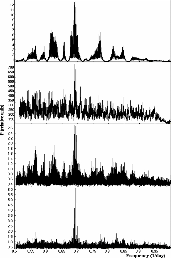
Figure 1. Power spectra of the variation of (from top to bottom) (1) stellar V magnitude of WD 1953−011 obtained from our observations (discussed in this paper), (2) stellar V magnitude of WD 1953−011 obtained from our observations together with those obtained by Brinkworth et al. (2005), (3) normalized Hα and Hβ EWs obtained from all available spectroscopic observations of WD 1953−011 (i.e., from the observations discussed in this paper, from data of Maxted et al. 2000, and from our previous observations presented by Valyavin et al. 2008), and (4) normalized residual intensities of the Hα and Hβ lines obtained from all available spectroscopic observations of the degenerate.
Download figure:
Standard image High-resolution imageDetailed study of the periodograms has shown that the most significant and sinusoidal signal common to all observables corresponds to a period of P = 1.441788(6) days. This period is very close to P = 1.441769 days found by Brinkworth et al. (2005) from their photometry. Due to this agreement, here we choose this period for phasing of all the data with the following ephemeris (for which JD0 corresponds to the maximum of the light variation):

4.2. Phase-resolved Photometry Against Zeeman Spectroscopy
In Figure 2 we illustrate the phase variations of the photometric magnitude (the upper two panels on the figure), EW of the Balmer lines (the third panel from top), and residual intensity rc of the lines. All the data are phased with the ephemeris described above. The lower two plots present the phase variation of the degenerate's global surface magnetic field (BG: mean field modulus integrated over the disk) with the same ephemeris and the projected fractional area S of the strong-field area on the disk (given in percentage of the full disk area). These data are taken from Valyavin et al. (2008) and re-phased with the current ephemeris. The two vertical dashed lines in Figure 2 correspond to those phases (ϕ ≈ 0.5; 1.5) when the star exhibits the minimum brightness, and therefore maximum projection of the dark area onto the disk.
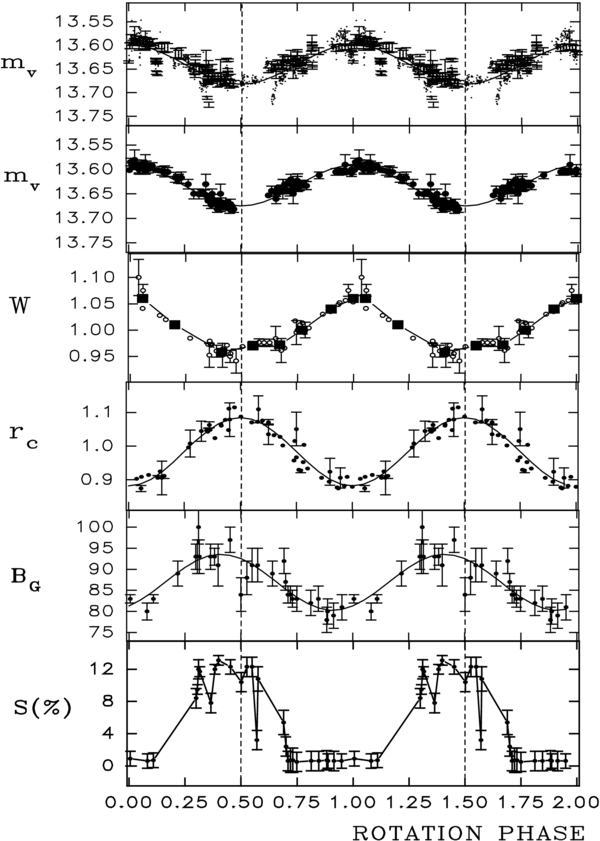
Figure 2. Phase variations with rotation period P = 1.441788(6) days of (from top to bottom) (1) stellar V magnitude of WD 1953−011 obtained from our observations together with those obtained by Brinkworth et al. (2005), (2) stellar V magnitude of the degenerate obtained from our observations only, (3) normalized Hα and Hβ EWs obtained from all available spectroscopic observations of WD 1953−011 (i.e., from the observations discussed in this paper, from data of Maxted et al. 2000, and from our previous observations presented by Valyavin et al. 2008), (4) normalized residual intensities of the Hα and Hβ lines obtained from all available spectroscopic observations of the degenerate, (5) global magnetic field of the degenerate, and (6) the projected fractional area of the strong-field area on the disk (the data are taken from Valyavin et al. 2008 and given in percentages of full disk square). The solid sinusoidal lines at plots 1, 2, 4, 5 (from top to bottom) are least-square fits of the data. The solid squares at the middle plot 3 are averaged data in bins. The two vertical solid lines pass through phases 0.5; 1.5. These phases correspond to minimum light energy from the star and maximum projection of the magnetic spot to the line of sight.
Download figure:
Standard image High-resolution imageAs can be seen from Figure 2, the spectroscopic observable rc also tends to have the smallest values at the phases of the light minimum. According to the above explanations this suggests a direct relationship between the dark area and strong-field spot. However, in comparison with the behavior of the residual intensity, the variation of EW demonstrates a non-sinusoidal shape with its absolute minimum shifted by Δϕ ≈ −0.05 relative to the phase of the light minimum (ϕ = 0.5). Averaging EW in the phase bins 0.41 < ϕ < 0.47 and 0.5 < ϕ < 0.55 and calculating the gradient of the data between these two phases, we have the formal absolute minimum of the EW change to be at ϕ ≈ 0.44 ± 0.017. Further, phased results of direct measurements of the projected area S (for details, see Section 4.2 and Table 3 in Valyavin et al. 2008) of the strong-magnetic spot on the disk seem to have the similar tendency, shifted in phase by this value. Because of this we shall discuss this phenomenon in the present study in more detail.
This phase shift was first observed by Wade et al. (2003) in their study of WD 1953−011 where they also estimated the "visibility" of the strong-magnetic area via analysis of Hα EWs. This shift could be produced by the presence of some morphologic difference in the distribution of the field and photometric flux intensities within the corresponding spots. Although the origin of the shift could be artificial due to uncertainties in our simplifying assumption that the variation of EWs of the Balmer line profiles is attributed to the strong-magnetic area only. The shift is, however, weak. And the general behavior of all the observables related to the dark and strong-field magnetic areas exhibits correlated behavior suggesting their geometric relationship.
Taking all of the above into account, we suppose that the dark and magnetic spots are physically connected. In order to illustrate this conclusion, below we model the dark spot from photometry comparing it with the geometry of the strong-field area obtained by Valyavin et al. (2008).
4.3. Modeling the Dark/Temperature Spot
In our model we assume that the star's flux variation is due to surface inhomogeneity in the temperature distribution. Assuming a black body relationship between temperature and energy flux we have
where h, c, and k are the Plank constant, speed of light, and Boltzmann constant; λv is wavelength centered at the V-band filter; FV and  are individual and averaged (over the entire rotational cycle) photometric fluxes, while Teff and
  are individual and averaged effective temperatures, respectively. Taking
  from our data,
  K (Bergeron et al. 2001), assuming that
  and weighting the visible Teff by the line-of-sight flow of radiation as an average mean of the local surface temperatures T(θ, ϕ), we obtain the following approximation equation:
where θ and ϕ are the spherical angles relative to the rotational axis of the star,  is the cosine of the angle between the surface element normal and the line of sight, and u is the limb darkening. For every square element, this cosine can be determined via the inclination i of the rotational axis with respect to the line-of-sight coordinates θ, ϕ of the square, and rotation phase f as follows:

In the integration procedure we assume negative  to be zero in order to integrate only over the visible hemisphere. Assuming a linear limb-darkening law and dividing the sphere by the elementary angles Δθ, Δϕ, Equation (2) can be rewritten as

where
Here, index k corresponds to an observed rotation phase, and l, n run latitudinal and longitudinal positions of the elementary squares in the star's rotational coordinate system.
Applying all available photometric observations covering the full rotation cycle, Equation (2) can be solved by using any of the nonlinear least-square methods if the angle i is known. In our model we used an inclination of i = 18° as determined by Valyavin et al. (2008). With the limb darkening u = 0.45, the temperature distribution up to 60 surface elements was calculated as presented below.
A general application of Equation (4) to the analysis of nearly sinusoidal signals provides more than a single solution, including physically unrealistic ones (negative surface temperatures, for example). In order to restrict the range of possible solutions for surface temperatures, we modified the temperatures to have the following parameterized form

where F(x) is a positive function of the parameter x and T0 is a physically reasonable lower temperature limit (say at the center of the coolest area). To choose a reasonable F(x) we tested several power, polynomial, and exponential functions. Finally, the simplest case F(x) = x2 was chosen. This case provides satisfactory convergence of Equation (4) if T0 is fixed.
In such a formulation Equation (4) was evaluated using the Marquardt χ2 minimization method (Bevington 1969). In our solution we minimize the function:

The used algorithm in FORTRAN-77 is presented by Press et al. (1992).
4.4. Model Results
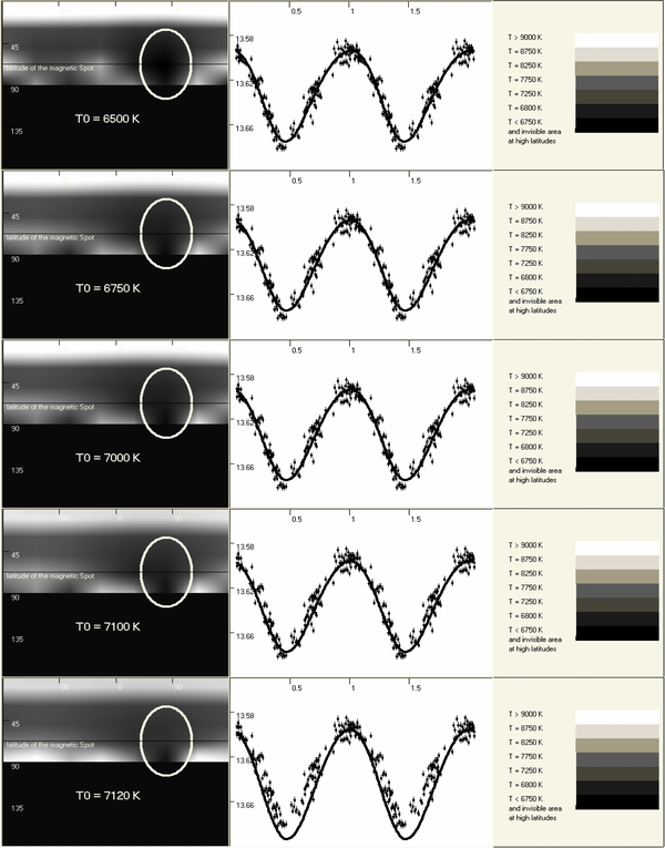
In Figure 3 we illustrate the tomographic portraits (left panels) of the resulting smoothed temperature distribution patterns in comparison to the strong-magnetic area. Dark areas correspond to low temperatures and brighter areas are higher temperatures. In these plots, the vertical axis is latitude, the horizontal axis is longitude. The longitude is presented from −180° to +180°. Middle panels are the corresponding phase light curves (solid lines) obtained from the model fits of the photometric observations (filled circles): vertical axis is mV, horizontal axis is rotation phase. Right panels illustrate in gray scale the temperature distribution in the tomographic portraits. Five examples of the star's temperature distribution with different T0 are illustrated (from top to bottom T0 = 6500 K, 6750 K, 7000 K, 7100 K, 7120 K). The strong-field spot is schematically illustrated in Figure 3 by the elliptical area bordered by a white solid line.
Figure 3. Examples of the tomographic portraits (left panels) of the star's temperature distribution in planar projections: vertical axis is latitude, horizontal axis is longitude. The longitude is presented from −180° to +180°. Middle panels are the corresponding phase light curves (solid lines) obtained from model fits of the photometric observations (filled circles): vertical axis is mV, horizontal axis is rotation phase. Right panels illustrate the explanation to the gray scale for the temperature distribution in the tomographic portraits. Five examples of the star's temperature distribution with different T0 are illustrated (from top to bottom T0 = 6500 K, 6750 K, 7000 K, 7100 K, 7120 K).
Download figure:
Standard image High-resolution image
All the illustrated solutions demonstrate two characteristic features: the presence of a temperature gradient from the rotation pole to the equator as well as the presence of a large low-temperature spot (the shadow) covering 15%–20% of the star's hemisphere. The size of the shadow corresponds well to the size of the strong-field area estimated by Valyavin et al. (2008). Three solutions at the lower temperature limits T0 = 6500 K, T0 = 6750 K, and T0 = 7000 K (the upper three plots in Figure 3) present the most stable fits of the data revealing temperature changes around the latitude of the strong-field area location (θ ≈ 67°). Higher temperature limits shift the shadow to upper latitudes and provide less robust fits to the photometric data (see the lower two plots in Figure 3). From consideration of all the solutions, we give the characteristic value to the lower temperature limit (the temperature at the center of the shadow) to be between 6000 K and 7000 K.
In order to find simpler solutions for the temperature distribution we also examined i as a parameter. The most stable and physically reasonable solutions are found within the range 10° ⩽ i ⩽ 20°. Within this range the tomographic portraits demonstrate similar features and temperature contrasts as discussed above.
The phase shift discussed previously (ϕ ≈ 0.05–0.1) might be produced by a longitudinal shift between the dark and magnetic spots of about 20°, and certainly not higher than 40°. However, even in these extreme cases the dark and strong-magnetic areas are overlapped by more than 60%. We therefore suggest that the dark and magnetic spots are indeed physically connected.
The small difference in phasing of the corresponding observables (mV and S in Figure 2) can also be explained by the following obvious fact. In our previous investigation of WD 1953−011 (Valyavin et al. 2008) where we determined the rotationally modulated projection S of the strong-field area to the line of sight, we assumed a constant temperature everywhere over the surface. Taking into account that the center of the low-temperature region may have an effective temperature about 20% below the mean effective temperature of the photosphere, we may suspect that these coolest parts of the surface may be undetectable spectroscopically in the integrated hydrogen spectrum of the degenerate. This could affect our analysis of the position of the strong-field area and produce a small artificial shift in the position of the strong-magnetic area.
The presence of the global gradient between the rotation pole to equator is also a remarkable result. We find this gradient from practically all tested T0. The cases of T0 ≈ 7100 K provide smaller values of the gradient. Lower values of T0 increase it. Also, testing smaller i (11° ⩽ i ⩽ 14°) we found some solutions with the smallest, but nevertheless non-zero gradient. In all cases, the presence of the gradient makes the shadow area have more diffusive edges, giving a smaller contrast in temperatures between the shadow and neighboring areas. In this paper, however, we are not making conclusions about the existence of the gradient, but only discuss the implications.
5. DISCUSSION
We have presented new photometric and spectral observations of the magnetic white dwarf WD 1953−011. From these observations and those published previously we have re-determined the star's rotation period, and studied the relationship between the brightness variation and the variation of the strong-magnetic spot projection. We find a new period of P = 1.441788(6) days. This period is consistent with all the observables we employed, including those associated with the global magnetic field.
From direct comparison of the phased photometric and spectroscopic observations, we have found that the extremum of the photometric variations of the V-band flux and extremum of varying projection of the magnetic spot to the line of sight are shifted relative to each other with phase shift of about 0.05–0.1. To study this shift we resolved the phase brightness variation of the star assuming a thermal origin of the photometric variability. We obtained a number of solutions which support the idea that the variability comes from a low-temperature dark spot covering about 15%–20% of the star's surface. The spot might have a temperature characteristically lower than the mean by a factor of about 20%.
Comparing positions of the strong-magnetic area and dark spot, we conclude that they are located at the same latitudes, significantly overlapping each other with a possible slight longitudinal shift that may be responsible for the phase shift discussed above. Given that the determination of the degenerate's strong-field area position and geometry given by Valyavin et al. (2008) were based on the assumption of constant effective temperature in the atmosphere of WD 1953−011, we propose that the observed shift may be a consequence of these assumptions. Besides, the total behavior of all the observables related to the dark and magnetic spots at other phases are generally well correlated within the error bars (see Figure 2). Due to these arguments, we suggest that the association between the dark spot and strong-field area in WD1953−011 is real.
The established association leads to the fundamental problem related to the origin and evolution of localized magnetic flux tubes in isolated white dwarfs (see discussions in Brinkworth et al. 2005; Valyavin et al. 2008). This idea, however, requires additional observational evidence such as the presence of secular drift of the tube which is still not established in WD 1953−011. In this context, we note that an independent search for the period using only the data related to the global component of the star's magnetic field provides much better phasing with a sightly longer period P = 1.448 days (Valyavin et al. 2008). This period contradicts all the other observables related to strong-magnetic and dark spots. Therefore, this may admit the possibility that the strong-magnetic area might slowly migrate over the star's surface.
The difference between the periods discussed above could be, in principle, explained by the presence of a slow drift of the strong-magnetic area relative to the star's global magnetic field with a characteristic time of about 280 days. This proposal, however, still requires additional low-resolution spectropolarimetric or high-resolution spectral observations of the global field in WD 1853−011.
Alternatively, in contrast to the idea of a low-temperature localized magnetic flux tube, we might assume that the brightness/temperature distribution pattern in WD 1953−011 may have a correlation with the global field intensity distribution, i.e., all local temperatures in WD 1953−011 correlate with corresponding local field intensities. In that case, the detected dark spot is just the coolest part of the general temperature distribution associated with the strongest magnetic features. This case might imply that there is a common, ordered anisotropy of the light energy transfer in atmospheres of magnetic degenerate stars due to the influence of their global magnetic fields. Such a phenomenon would not be new for degenerate stars. For example, it was discussed in application to neutron stars by Page & Sarmiento (1996). For the magnetic white dwarfs, however, such a phenomenon has not been observed until now.
Our thanks to L. Ferrario, P. Maxted, and C. Brinkworth for providing details of individual spectroscopic and photometric measurements of WD 1953−011. We are also especially grateful to our anonymous referee for valuable comments and suggestions. G.A.W. acknowledges Discovery Grant support from the Natural Sciences and Engineering Research Council of Canada. I.H. thanks KFICST (grant 07-179). S.P. acknowledges support from the Ukrainian Fundamental Research State Fund (M/364) and the Austrian Science Fund (P17890). L.F.M. and M.A. acknowledge financial support from the UNAM via PAPIIT grant IN114309. D.S. acknowledges financial support from Deutsche Forschungsgemeinschaft (DFG), Research Grant RE1664/7-1, and FWF Lise Meitner grant Nr. M998-N16.
Footnotes
- 11
Due to weather conditions, in these cases we had to average the data within about 5000 s equivalent exposure bins; see Table 2.